R E S E A R C H
Open Access
A fitted numerical scheme for second
order singularly perturbed delay differential
equations via cubic spline in compression
Podila Pramod Chakravarthy
1*, S Dinesh Kumar
1, Ragi Nageshwar Rao
2and Devendra P Ghate
3*Correspondence:
[email protected] 1Department of Mathematics,
Visvesvaraya National Institute of Technology, Nagpur, 440010, India Full list of author information is available at the end of the article
Abstract
This paper deals with the singularly perturbed boundary value problem for the
second order delay differential equation. Similar boundary value problems are
associated with expected first-exit times of the membrane potential in models of
neurons. An exponentially fitted difference scheme on a uniform mesh is
accomplished by the method based on cubic spline in compression. The difference
scheme is shown to converge to the continuous solution uniformly with respect to
the perturbation parameter, which is illustrated with numerical results.
Keywords:
singular perturbations; cubic spline in compression; boundary layer;
delay differential equation; exponentially fitted finite difference method
1 Background
In the last few decades there has been a growing interest in the study of delay
differen-tial equations due to their occurrence in a wide variety of application fields such as
bio-sciences, control theory, economics, material science, medicine, robotics
etc
. Any system
involving a feedback control will almost always involve time delays. These arise because
a finite time is required to sense the information and then to react to it. The delays or
lags can represent gestation times, incubation periods, transport delays
etc
. Delay
mod-els are also prominent in describing several aspects of infectious disease dynamics such
as primary infection, drug therapy, immune response
etc
. Delays have also appeared in
the study of chemostat models, circadian rhythms, epidemiology, the respiratory system,
tumor growth and neural networks. Statistical analysis of ecological data has shown that
there is evidence of delay effects in the population dynamics of many species.
The details of the theory and applications of differential difference equations can be
found in the collection of books, to name a few, Bellman and Cooke [], Driver [], El’sgol’ts
and Norkin [], Erneux [], Gopalsamy [], Györi and Ladas [], Halanay [], Kuang []
and Smith []. In recent years there has been a growing interest in the numerical study
of differential difference equations. However, the first discrete solution to delay
differ-ential equations was given by Feldstein [], which became a landmark work to most of
the researchers working in numerical analysis of delay differential equations. Bellen and
Zennaro [] gave the theoretical aspects of numerical methods for ordinary and delay
dif-ferential equations, and suitable techniques for solving numerically such type of equations.
A singularly perturbed delay differential equation is a differential equation in which the
highest derivative is multiplied by a small parameter and which involves at least one shift
term. Such problems arise frequently in the mathematical modeling of various physical
and biological phenomena like optically bistable devices [, ], description of the human
pupil reflex [], a variety of models for physiological processes or diseases [], variational
problems in control theory [, ] and the first-exit time problem in the modeling of the
activation of neuronal variability [].
Singularly perturbed delay differential equations have up to now not been satisfactorily
discussed in numerical analysis literature; however, in recent years there has been a
grow-ing interest in the numerical study of such problems. Most of the previous works have
been centered on the existence and uniqueness of solutions for initial value problems in
differential difference equations and very little attention has been paid to construction of
approximate solutions. The computation of the solution of delay differential equations has
been a great challenge and great importance due to the appearance of such equations in
mathematical modeling of biological problems. Stein [] approximated the solution of
his model of the activation of neuronal variability, which was studied by Tuckwell [–]
and by Wilbur and Rinzel []. Lange and Miura [–] gave a series of papers on
sin-gularly perturbed differential difference equations by extending the matched asymptotic
expansion approach developed for ordinary differential equations to obtain the
approxi-mate solution of these differential difference equations. An extensive numerical work has
been initiated by Kadalbajoo and Sharma in their papers [–], Kadalbajoo and Kumar
[], Kadalbajoo and Ramesh []. Gulsu and Sezer [] proposed a Taylor polynomial
approach for solving
m
th order linear differential difference equations with mixed
condi-tions. This method is based on first taking the truncated Taylor’s expansions of the
func-tions in the differential difference equafunc-tions and then substituting their matrix forms into
the equation. Hence the resultant matrix equation can be solved and the unknown Taylor
coefficients can be found approximately.
It is well known that standard discretization methods for solving singular perturbation
problems are unstable and fail to give accurate results when the perturbation parameter
ε
is small. Therefore it is important to develop suitable numerical methods to deal with
these problems whose accuracy does not depend on the parameter value
ε
. So the method
should be uniformly convergent with respect to the perturbation parameter, and various
approaches for the numerical methods to solve singularly perturbed differential equations
are given in [–]. The use of cubic splines for the solution of linear two point boundary
value problems was suggested by Bickley []. Aziz and Khan [] proposed a method
based on cubic spline in compression for the linear second order singularly perturbed
problems which have second and fourth order convergence depending on the choice of
the parameters
λ
and
λ
involved in the method.
The analytical and numerical solution of singularly perturbed delay differential
equa-tions with large delays can be found in Amiraliyev and Erdogan [], Amiraliyev and
Cimen [], Amiraliyeva
et al
. [], Erdogan and Amiraliyev []. Subburayan and
differential equations and delay systems with inverse delay that models these problems.
A direct algorithm is given for solving this problem. The delay function and inverse time
function are expanded by the Bezier curves. The Bezier curves are chosen as piecewise
polynomials of degree
n
, and the Bezier curves are determined on any subinterval by
n
+
control points. The approximated solution of delay systems containing inverse time is
derived.
In this paper, we propose a scheme based on cubic spline in compression which
com-prises an exponentially fitted difference scheme on a uniform mesh. In Section , we state
some important properties of the exact solution. In Section , we describe a difference
scheme based on cubic spline in compression for a second order singularly perturbed
de-lay differential equation. In Section , we give the numerical algorithm to solve a singularly
perturbed delay differential equation. Some numerical results are presented in Section ,
and conclusions are given in Section .
2 Statement of the problem
We consider the following boundary value problem (BVP) for the delay differential
equa-tion (DDE):
ε
y
(
x
) +
a
(
x
)
y
(
x
) +
b
(
x
)
y
(
x
– ) =
f
(
x
),
<
x
< ,
()
subject to the interval and boundary conditions
y
(
x
) =
φ
(
x
),
x
∈
[–, ];
y
() =
β
,
()
where <
ε
and
a
(
x
)
≥
α
> ,
a
(
x
),
b
(
x
),
f
(
x
) are given sufficiently smooth functions on
[, ],
φ
(
x
) is a smooth function on [–, ] and
β
is a given constant which is independent
of
ε
, the boundary value problem () along with () exhibits a strong boundary layer at
x
= (
cf.
[], p.).
If
a
(
x
) < ,
a
(
x
),
b
(
x
),
f
(
x
) are given sufficiently smooth functions on [, ],
φ
(
x
) is a
smooth function on [–, ] and
β
is a given constant which is independent of
ε
, then the
boundary value problem () along with () exhibits a strong boundary layer at
x
= (
cf.
[], p.).
2.1 Stability result
Here we show some properties of the solution of () and (). We use the following
conven-tion:
g
∞=
max
≤x≤
g
(
x
)
,
g
=
g
(
x
)
dx
,
g
∞,=
g
(
x
)
dx
,
g
∞,=
g
(
x
)
dx
and
g
=
–
g
(
x
)
dx
.
Lemma
If a
(
x
),
b
(
x
),
f
(
x
)
∈
C
[, ]
and
φ
(
x
)
∈
C
[–, ]
and
ρ
=
α
–b
∞,< ,
then the
solution y
(
x
)
of problem
()
and
()
follows the estimates
y
(
x
)
≤
C
Proof
From () we have
y
(
x
) =
y
()
e
–εSubstituting () in (), we get
equation () can be rewritten as
Alternatively the Green’s function of the operator
≤
φ
()
+
|
β
|
+
α
–Now we prove estimate ().
Since
Consider from () that we have
≤
α
–f
+
α
–b
∞,φ
+
α
–b
∞,C
≡
C
.
Substituting this in (), we get
y
()
≤
|
β
|
+
|
φ
()
|
+
εUsing the procedure in (), we get
y
(
x
)
≤
C
3 Derivation of the method
Let
x
= ,
x
N= ,
x
i=
ih
,
h
= /
N
.
Solving () as a linear second order differential equation, we get
s
(
x
i) =
A
cos
We can find the arbitrary constants
A
and
B
by using interpolatory conditions
Differentiating equation () and equating the left- and right-hand derivatives at
x
i, we
have
y
i–
y
i–h
+
h
λ
( –
λ
cot
λ
)
M
i–
–
λ
sin
λ
M
i–=
y
i+–
y
ih
+
h
λ
–
λ
sin
λ
M
i+– ( –
λ
cot
λ
)
M
i.
()
This leads to a tridiagonal system
h
(
λ
M
i–+
λ
M
i+
λ
M
i+) =
y
i+–
y
i+
y
i–,
i
= , , . . . ,
N
– ,
()
where
λ
=
λ
λ
sin
λ
–
,
λ
=
λ
( –
λ
cot
λ
).
The condition of continuity given by () ensures the continuity of first order derivatives
of the spline
s
(
x
,
τ
) at interior points.
Substituting,
ε
M
i= –
a
(
x
i)
y
i–
b
(
x
i)
y
(
x
i–)+
f
(
x
i) in equation () and using the following
approximations for first order derivative of
y
:
y
i∼
=
(
y
i+–
y
i–)
h
,
y
i+∼
=
(
y
i+–
y
i+
y
i–)
h
,
y
i–∼
=
(–
y
i++
y
i–
y
i–)
h
,
we get the following tridiagonal linear system:
–
ε
+
λ
ha
i–+
λ
ha
i–
λ
ha
i+y
i–+ (
ε
–
λ
ha
i–+
λ
ha
i+)
y
i+
–
ε
+
λ
ha
i––
λ
ha
i–
λ
ha
i+y
i+= –
h
λ
(
f
i––
b
i–y
i––N) +
λ
(
f
i–
b
iy
i–N)
+
λ
(
f
i+–
b
i+y
i+–N)
,
i
= , , . . . ,
N
– .
()
4 Numerical algorithm
Step
. We obtain the reduced problem by setting
ε
= in equation () with an appropriate
interval condition. Let
y
(
x
) be the solution of the reduced problem of () and (),
i.e.
,
a
(
x
)
y
(
x
) +
b
(
x
)
y
(
x
– ) =
f
(
x
)
()
with
y
(
x
) =
φ
(
x
),
–
≤
x
≤
.
()
We consider
y
() =
γ
.
Step
. To obtain the solution in <
x
< , we consider the numerical scheme from ()
with a fitting factor
σ
(
ρ
) =
a
iρ
Coth
a
iρ
,
where
ρ
=
h
ε
(
cf.
[]).
Scheme () with a fitting factor can be written as
E
iy
i––
F
iy
i+
G
iy
i+=
H
i,
<
i
<
N
– ,
where
E
i= –
εσ
+
λ
ha
i–+
λ
ha
i–
λ
ha
i+,
F
i= –(
εσ
–
λ
ha
i–+
λ
ha
i+),
G
i= –
εσ
+
λ
ha
i––
λ
ha
i–
λ
ha
i+and
H
i= –
h
λ
(
f
i––
b
i–φ
i––N) +
λ
(
f
i–
b
iφ
i–N) +
λ
(
f
i+–
b
i+φ
i+–N)
.
We solve this system by Thomas algorithm with the boundary conditions
y
=
φ
()
and
y
N=
γ
.
Similarly, to obtain the solution in <
x
< , we rewrite the numerical scheme with the
fitting factor as:
E
iy
i––
F
iy
i+
G
iy
i+=
H
i,
N
+ <
i
<
N
– ,
where
E
i= –
εσ
+
λ
ha
i–+
λ
ha
i–
λ
ha
i+,
F
i= –(
εσ
–
λ
ha
i–+
λ
ha
i+),
G
i= –
εσ
+
λ
ha
i––
λ
ha
i–
λ
ha
i+and
H
i= –
h
λ
(
f
i––
b
i–y
i––N) +
λ
(
f
i–
b
iy
i–N) +
λ
(
f
i+–
b
i+y
i+–N)
.
We solve the system with the boundary conditions
y
N=
γ
and
y
N=
β
.
5 Numerical examples
To demonstrate the applicability of the method, we consider one boundary value
prob-lem of singularly perturbed linear differential difference equations exhibiting boundary
layer at the left end of the interval [, ] and four boundary value problems with right-end
boundary layer. These problems were widely discussed in the literature. The numerical
results are presented for
λ
=
,
λ
=
.
Since the exact solutions of the problems are not known, the maximum absolute errors
for the examples are calculated using the following double mesh principle:
E
Nε=
max
For a value of
N
, the
ε
-uniform maximum absolute error is calculated by the formula
E
N=
max
ε
E
εN.
The numerical rate of convergence for all the examples has been calculated by the
for-mula
R
N=
log
|
E
N ε/
E
εN|
log
.
Example
([], p.)
ε
y
(
x
) +
y
(
x
) + .
y
(
x
– ) = .(
x
– ), <
x
<
,
y
(
x
) =
x
,
–
≤
x
≤
,
y
(
) = .
The numerical results are presented in Table for different vales of perturbation
param-eter
ε
.
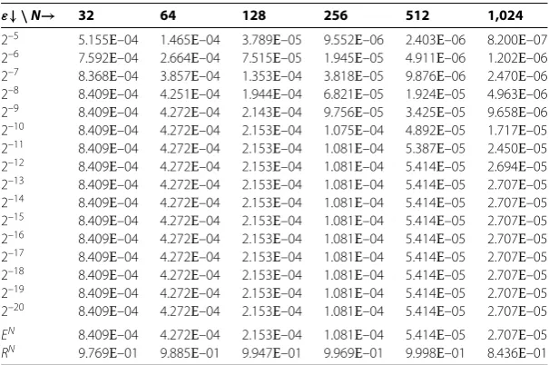
Example
([], p.)
ε
y
(
x
) –
y
(
x
) +
y
(
x
– ) = ,
y
(
x
) = , –
≤
x
≤
,
y
() = .
Table 1 The maximum absolute errors for Example 1 for different values of
ε
ε↓ \N→ 32 64 128 256 512 1,024
2–5 1.017E–05 5.086E–06 2.543E–06 1.272E–06 6.358E–07 1.967E–06 2–6 1.017E–05 5.086E–06 2.543E–06 1.272E–06 6.358E–07 7.480E–07
2–7 1.017E–05 5.086E–06 2.543E–06 1.272E–06 6.358E–07 5.579E–07
2–8 1.017E–05 5.086E–06 2.543E–06 1.272E–06 6.358E–07 5.544E–07
2–9 1.017E–05 5.086E–06 2.543E–06 1.272E–06 6.358E–07 5.544E–07
2–10 1.017E–05 5.086E–06 2.543E–06 1.272E–06 6.358E–07 5.544E–07
2–11 1.017E–05 5.086E–06 2.543E–06 1.272E–06 6.358E–07 5.544E–07
2–12 1.017E–05 5.086E–06 2.543E–06 1.272E–06 6.358E–07 5.544E–07
2–13 1.017E–05 5.086E–06 2.543E–06 1.272E–06 6.358E–07 5.544E–07
2–14 1.017E–05 5.086E–06 2.543E–06 1.272E–06 6.358E–07 5.544E–07
2–15 1.017E–05 5.086E–06 2.543E–06 1.272E–06 6.358E–07 5.544E–07
2–16 1.017E–05 5.086E–06 2.543E–06 1.272E–06 6.358E–07 5.544E–07
2–17 1.017E–05 5.086E–06 2.543E–06 1.272E–06 6.358E–07 5.544E–07
2–18 1.017E–05 5.086E–06 2.543E–06 1.272E–06 6.358E–07 5.544E–07
2–19 1.017E–05 5.086E–06 2.543E–06 1.272E–06 6.358E–07 5.544E–07
2–20 1.017E–05 5.086E–06 2.543E–06 1.272E–06 6.358E–07 5.544E–07
EN 1.017E–05 5.086E–06 2.543E–06 1.272E–06 6.358E–07 5.544E–07 RN 1.000E+00 1.000E+00 1.000E+00 1.000E+00 1.976E–01 1.284E+00
Table 2 The maximum absolute errors for Example 2 for different values of
ε
ε↓ \N→ 32 64 128 256 512 1,024
2–5 5.155E–04 1.465E–04 3.789E–05 9.552E–06 2.403E–06 8.200E–07
2–6 7.592E–04 2.664E–04 7.515E–05 1.945E–05 4.911E–06 1.202E–06
2–7 8.368E–04 3.857E–04 1.353E–04 3.818E–05 9.876E–06 2.470E–06
2–8 8.409E–04 4.251E–04 1.944E–04 6.821E–05 1.924E–05 4.963E–06
2–9 8.409E–04 4.272E–04 2.143E–04 9.756E–05 3.425E–05 9.658E–06
2–10 8.409E–04 4.272E–04 2.153E–04 1.075E–04 4.892E–05 1.717E–05
2–11 8.409E–04 4.272E–04 2.153E–04 1.081E–04 5.387E–05 2.450E–05
2–12 8.409E–04 4.272E–04 2.153E–04 1.081E–04 5.414E–05 2.694E–05
2–13 8.409E–04 4.272E–04 2.153E–04 1.081E–04 5.414E–05 2.707E–05
2–14 8.409E–04 4.272E–04 2.153E–04 1.081E–04 5.414E–05 2.707E–05 2–15 8.409E–04 4.272E–04 2.153E–04 1.081E–04 5.414E–05 2.707E–05 2–16 8.409E–04 4.272E–04 2.153E–04 1.081E–04 5.414E–05 2.707E–05 2–17 8.409E–04 4.272E–04 2.153E–04 1.081E–04 5.414E–05 2.707E–05 2–18 8.409E–04 4.272E–04 2.153E–04 1.081E–04 5.414E–05 2.707E–05 2–19 8.409E–04 4.272E–04 2.153E–04 1.081E–04 5.414E–05 2.707E–05
2–20 8.409E–04 4.272E–04 2.153E–04 1.081E–04 5.414E–05 2.707E–05
Table 3 The maximum absolute errors for Example 3 for different values of
ε
ε↓ \N→ 32 64 128 256 512 1,024
2–5 2.074E–02 5.496E–03 1.395E–03 3.503E–04 8.744E–05 4.587E–05 2–6 3.534E–02 1.073E–02 2.853E–03 7.243E–04 1.816E–04 6.401E–05 2–7 4.558E–02 1.801E–02 5.495E–03 1.456E–03 3.697E–04 1.040E–04 2–8 4.727E–02 2.316E–02 9.148E–03 2.781E–03 7.368E–04 1.916E–04 2–9 4.730E–02 2.402E–02 1.167E–02 4.611E–03 1.399E–03 3.722E–04
2–10 4.730E–02 2.403E–02 1.210E–02 5.860E–03 2.314E–03 7.028E–04
2–11 4.730E–02 2.403E–02 1.211E–02 6.076E–03 2.935E–03 1.160E–03
2–12 4.730E–02 2.403E–02 1.211E–02 6.080E–03 3.044E–03 1.473E–03
2–13 4.730E–02 2.403E–02 1.211E–02 6.080E–03 3.046E–03 1.526E–03
2–14 4.730E–02 2.403E–02 1.211E–02 6.080E–03 3.046E–03 1.527E–03
2–15 4.730E–02 2.403E–02 1.211E–02 6.080E–03 3.046E–03 1.527E–03
2–16 4.730E–02 2.403E–02 1.211E–02 6.080E–03 3.046E–03 1.527E–03
2–17 4.730E–02 2.403E–02 1.211E–02 6.080E–03 3.046E–03 1.527E–03
2–18 4.730E–02 2.403E–02 1.211E–02 6.080E–03 3.046E–03 1.527E–03
2–19 4.730E–02 2.403E–02 1.211E–02 6.080E–03 3.046E–03 1.527E–03
2–20 4.730E–02 2.403E–02 1.211E–02 6.080E–03 3.046E–03 1.527E–03
EN 4.730E–02 2.403E–02 1.211E–02 6.080E–03 3.046E–03 1.527E–03 RN 9.769E–01 9.886E–01 9.941E–01 9.972E–01 9.965E–01 1.002E+00
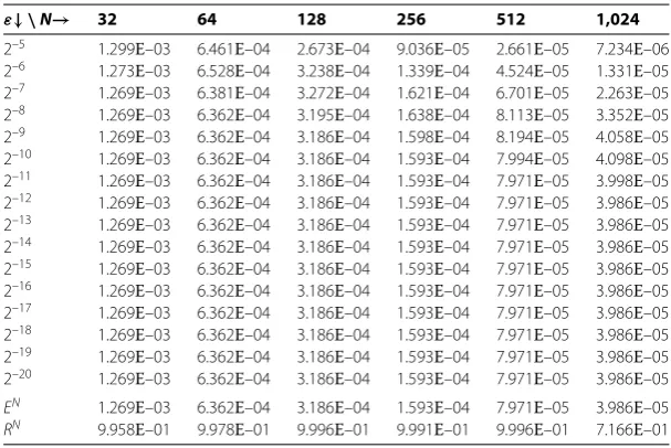
Table 4 The maximum absolute errors for Example 4 for different values of
ε
ε↓ \N→ 32 64 128 256 512 1,024
2–5 1.299E–03 6.461E–04 2.673E–04 9.036E–05 2.661E–05 7.234E–06
2–6 1.273E–03 6.528E–04 3.238E–04 1.339E–04 4.524E–05 1.331E–05
2–7 1.269E–03 6.381E–04 3.272E–04 1.621E–04 6.701E–05 2.263E–05
2–8 1.269E–03 6.362E–04 3.195E–04 1.638E–04 8.113E–05 3.352E–05
2–9 1.269E–03 6.362E–04 3.186E–04 1.598E–04 8.194E–05 4.058E–05
2–10 1.269E–03 6.362E–04 3.186E–04 1.593E–04 7.994E–05 4.098E–05
2–11 1.269E–03 6.362E–04 3.186E–04 1.593E–04 7.971E–05 3.998E–05
2–12 1.269E–03 6.362E–04 3.186E–04 1.593E–04 7.971E–05 3.986E–05
2–13 1.269E–03 6.362E–04 3.186E–04 1.593E–04 7.971E–05 3.986E–05 2–14 1.269E–03 6.362E–04 3.186E–04 1.593E–04 7.971E–05 3.986E–05 2–15 1.269E–03 6.362E–04 3.186E–04 1.593E–04 7.971E–05 3.986E–05 2–16 1.269E–03 6.362E–04 3.186E–04 1.593E–04 7.971E–05 3.986E–05 2–17 1.269E–03 6.362E–04 3.186E–04 1.593E–04 7.971E–05 3.986E–05
2–18 1.269E–03 6.362E–04 3.186E–04 1.593E–04 7.971E–05 3.986E–05
2–19 1.269E–03 6.362E–04 3.186E–04 1.593E–04 7.971E–05 3.986E–05
2–20 1.269E–03 6.362E–04 3.186E–04 1.593E–04 7.971E–05 3.986E–05
EN 1.269E–03 6.362E–04 3.186E–04 1.593E–04 7.971E–05 3.986E–05 RN 9.958E–01 9.978E–01 9.996E–01 9.991E–01 9.996E–01 7.166E–01
The numerical results are presented in Table for different vales of perturbation
pa-rameter
ε
.
Example
([], p.)
ε
y
(
x
) –
y
(
x
) +
y
(
x
– ) = ,
y
(
x
) = , –
≤
x
≤
,
y
() = .
The numerical results are presented in Table for different vales of perturbation
param-eter
ε
.
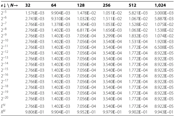
Example
([], p.)
ε
y
(
x
) –
y
(
x
) +
y
(
x
– ) =
,–, ≤≤xx≤≤,,y
(
x
) = , –
≤
x
≤
,
y
() = .
The numerical results are presented in Table for different vales of perturbation
pa-rameter
ε
.
Table 5 The maximum absolute errors for Example 5 for different values of
ε
ε↓ \N→ 32 64 128 256 512 1,024
2–5 1.576E–03 9.904E–03 1.478E–02 1.051E–02 5.821E–03 3.000E–03 2–6 2.743E–03 9.310E–04 1.032E–02 1.511E–02 1.067E–02 5.887E–03 2–7 2.766E–03 1.378E–03 1.304E–03 1.053E–02 1.528E–02 1.075E–02 2–8 2.766E–03 1.402E–03 6.817E–04 1.656E–03 1.063E–02 1.538E–02 2–9 2.766E–03 1.402E–03 7.056E–04 3.299E–04 1.832E–03 1.074E–02
2–10 2.766E–03 1.402E–03 7.056E–04 3.540E–04 1.531E–04 1.920E–03
2–11 2.766E–03 1.402E–03 7.056E–04 3.540E–04 1.772E–04 6.508E–05
2–12 2.766E–03 1.402E–03 7.056E–04 3.540E–04 1.772E–04 8.922E–05
2–13 2.766E–03 1.402E–03 7.056E–04 3.540E–04 1.772E–04 8.922E–05
2–14 2.766E–03 1.402E–03 7.056E–04 3.540E–04 1.772E–04 8.922E–05
2–15 2.766E–03 1.402E–03 7.056E–04 3.540E–04 1.772E–04 8.922E–05
2–16 2.766E–03 1.402E–03 7.056E–04 3.540E–04 1.772E–04 8.922E–05
2–17 2.766E–03 1.402E–03 7.056E–04 3.540E–04 1.772E–04 8.922E–05
2–18 2.766E–03 1.402E–03 7.056E–04 3.540E–04 1.772E–04 8.922E–05
2–19 2.766E–03 1.402E–03 7.056E–04 3.540E–04 1.772E–04 8.922E–05
2–20 2.766E–03 1.402E–03 7.056E–04 3.540E–04 1.772E–04 8.922E–05
EN 2.766E–03 1.402E–03 7.056E–04 3.540E–04 1.772E–04 8.922E–05 RN 9.806E–01 9.904E–01 9.952E–01 9.979E–01 9.902E–01 9.943E–01
The numerical results are presented in Table for different vales of perturbation
param-eter
ε
.
6 Discussion and conclusions
In this paper we present an exponentially fitted finite difference scheme to solve singularly
perturbed delay differential equation of second order with large delay. The method is based
on cubic spline in compression. We have implemented the present method on one linear
example with left-end boundary layer and four examples with right-end boundary layer by
taking different values of
ε
. Numerical results are presented in tables. From the results, it
can be observed that as the grid size
h
decreases, the maximum absolute errors decrease,
which shows the convergence to the computed solution. On the basis of the numerical
results of a variety of examples, it is concluded that the present method offers significant
advantage for the linear singularly perturbed delay differential equations with large delays.
Competing interests
The authors declare that they have no competing interests.
Authors’ contributions
All authors contributed equally to the writing of this paper. All authors read and approved the final manuscript.
Author details
1Department of Mathematics, Visvesvaraya National Institute of Technology, Nagpur, 440010, India.2School of Advanced
Sciences, VIT University, Vellore, Tamilnadu 632014, India.3Department of Aeronautical Engineering, ADCET, Sangli, Ashta, India.
Authors’ information
Acknowledgements
The authors wish to thank the National Board for Higher Mathematics, Department of Atomic Energy, Government of India, for their financial support under the project No. NBHM/R.P. 37/2012/Fresh/1742 dated 15th November, 2012. The authors are grateful to the referees for their careful reading of the manuscript and valuable comments. The authors thank for the help from the editor too.
Received: 22 May 2015 Accepted: 8 September 2015
References
1. Bellman, R, Cooke, KL: Differential-Difference Equations. Academic Press, New York (1963) 2. Driver, RD: Ordinary and Delay Differential Equations. Springer, New York (1977)
3. El’sgol’ts, LE, Norkin, SB: Introduction to the Theory and Application of Differential Equations with Deviating Arguments. Mathematics in Science and Engineering. Academic Press, San Diego (1973)
4. Erneux, T: Applied Delay Differential Equation. Springer, New York (2009)
5. Gopalsamy, K: Stability and Oscillations in Delay Differential Equations of Population Dynamics. Kluwer Academic, Dordrecht (1992)
6. Györi, I, Ladas, G: Oscillation Theory of Delay Equations with Applications. Clarendon, Oxford (1991) 7. Halanay, A: Differential Equations: Stability, Oscillations, Time Lags. Mathematics in Science and Engineering.
Academic Press, San Diego (1996)
8. Kuang, Y: Delay Differential Equations with Applications in Population Dynamics. Academic Press, New York (1993) 9. Smith, H: An Introduction to Delay Differential Equations with Applications to the Life Sciences. Springer, Berlin
(2010)
10. Feldstein, MA, Stetter, HJ: Simplified predictor-corrector methods. Numerical analysis research technical report, University of California, Los Angeles (1963)
11. Bellen, A, Zennaro, M: Numerical Methods for Delay Differential Equations. Oxford Science Publications, New York (2003)
12. Derstine, MW, Gibbs, FAHHM, Kaplan, DL: Bifurcation gap in a hybrid optical system. Phys. Rev. A26, 3720-3722 (1982) 13. Mallet-Paret, J, Nussbaum, RD: A differential-delay equations arising in optics and physiology. SIAM J. Math. Anal.20,
249-292 (1989)
14. Longtin, A, Milton, J: Complex oscillations in the human pupil light reflex with mixed and delayed feedback. Math. Biosci.90, 183-199 (1988)
15. Mackey, MC, Glass, L: Oscillation and chaos in physiological control systems. Science197, 287-289 (1977) 16. Glizer, VY: Asymptotic solution of a boundary-value problem for linear singularly-perturbed functional differential
equations arising in optimal control theory. J. Optim. Theory Appl.106, 309-335 (2000)
17. Glizer, VY: Blockwise estimate of the fundamental matrix of linear singularly perturbed differential systems with small delay and its application to uniform asymptotic solution. J. Math. Anal. Appl.278, 409-433 (2003)
18. Stein, RB: A theoretical analysis of neuronal variability. Biophys. J.5, 173-194 (1965)
19. Tuckwell, HC: On the first-exit time problem for temporally homogeneous Markov processes. J. Appl. Probab.13, 39-48 (1976)
20. Tuckwell, HC: Introduction to Theoretical Neurobiology, vol. 1. Cambridge University Press, Cambridge (1988) 21. Tuckwell, HC: Introduction to Theoretical Neurobiology, vol. 2. Cambridge University Press, Cambridge (1988) 22. Wilbur, WJ, Rinzel, J: An analysis of Stein’s model for stochastic neuronal excitation. Biol. Cybern.45, 107-114 (1982) 23. Lange, CG, Miura, RM: Singular perturbation analysis of boundary-value problems for differential-difference
equations. SIAM J. Appl. Math.42, 502-531 (1982)
24. Lange, CG, Miura, RM: Singular perturbation analysis of boundary-value problems for differential-difference equations. II. Rapid oscillations and resonances. SIAM J. Appl. Math.45, 687-707 (1985)
25. Lange, CG, Miura, RM: Singular perturbation analysis of boundary-value problems for differential-difference equations. III. Turning point problems. SIAM J. Appl. Math.45, 708-734 (1985)
26. Lange, CG, Miura, RM: Singular perturbation analysis of boundary value problems for differential difference equations. IV. A nonlinear example with layer behavior. Stud. Appl. Math.84, 231-273 (1991)
27. Lange, CG, Miura, RM: Singular perturbation analysis of boundary-value problems for differential-difference equations. V. Small shifts with layer behavior. SIAM J. Appl. Math.54, 249-272 (1994)
28. Lange, CG, Miura, RM: Singular perturbation analysis of boundary-value problems for differential-difference equations. VI. Small shifts with rapid oscillations. SIAM J. Appl. Math.54, 273-283 (1994)
29. Kadalbajoo, MK, Sharma, KK: Numerical analysis of boundary value problems for singularly perturbed differential difference equations with small shifts of mixed type. J. Optim. Theory Appl.115(1), 145-163 (2002)
30. Kadalbajoo, MK, Sharma, KK: Numerical analysis of singularly perturbed delay differential equations with layer behavior. Appl. Math. Comput.157, 11-28 (2004)
31. Kadalbajoo, MK, Sharma, KK: Numerical analysis of boundary value problems for singularly perturbed differential difference equations: small shifts of mixed type with rapid oscillations. Commun. Numer. Methods Eng.20, 167-182 (2004)
32. Kadalbajoo, MK, Sharma, KK:ε-Uniformly fitted mesh method for singularly perturbed differential difference equations: mixed type of shifts with layer behavior. Int. J. Comput. Math.81(1), 49-62 (2004)
33. Kadalbajoo, MK, Sharma, KK: Numerical treatment of a mathematical model arising from a model of neuronal variability. J. Math. Anal. Appl.307, 606-627 (2005)
34. Kadalbajoo, MK, Sharma, KK: Numerical treatment of boundary value problems for second order singularly perturbed delay differential equations. Comput. Appl. Math.24(2), 151-172 (2005)
35. Kadalbajoo, MK, Sharma, KK: Numerical treatment for singularly perturbed nonlinear differential difference equations with negative shift. Nonlinear Anal.63, e1909-e1924 (2005)
37. Kadalbajoo, MK, Sharma, KK: Anε-uniform convergent method for a general boundary value problem for singularly perturbed differential difference equations: small shifts of mixed type with layer behavior. J. Comput. Methods Sci. Eng.6(1), 39-55 (2006)
38. Kadalbajoo, MK, Sharma, KK: A numerical method based on finite difference for boundary value problems for singularly perturbed delay differential equations. Appl. Math. Comput.197, 692-707 (2008)
39. Kadalbajoo, MK, Kumar, D: A computational method for singularly perturbed nonlinear differential-difference equations with small shift. Appl. Math. Model.34, 2584-2596 (2010)
40. Kadalbajoo, MK, Ramesh, VP: Hybrid method for numerical solution of singularly perturbed delay differential equations. Appl. Math. Comput.187, 797-814 (2007)
41. Gulsu, M, Sezer, M: A Taylor polynomial approach for solving differential-difference equations. J. Comput. Appl. Math. 186, 349-364 (2006)
42. Doolan, ER, Miller, JJH, Schilders, WHA: Uniform Numerical Methods for Problems with Initial and Boundary Layers. Boole, Dublin (1980)
43. Miller, JJH, O’Riordan, E, Shiskin, GI: Fitted Numerical Methods for Singular Perturbation Problems. World Scientific, Singapore (1996)
44. Roos, HG, Stynes, M, Tobiska, L: Numerical Methods for Singularly Perturbed Differential Equations. Springer, Berlin (1996)
45. Farrell, PA, Hegarty, AF, Miller, JJH, O’Riordan, E, Shishkin, GI: Robust Computational Techniques for Boundary Layers. Chapman & Hall/CRC, New York (2000)
46. Bickley, WG: Piecewise cubic interpolation and two point boundary value problems. Comput. J.11, 206-208 (1968) 47. Aziz, T, Khan, A: A spline method for second order singularly perturbed boundary value problems. J. Comput. Appl.
Math.147, 445-452 (2002)
48. Amiraliyev, GM, Erdogan, F: Uniform numerical method for singularly perturbed delay differential equations. Comput. Math. Appl.53, 1251-1259 (2007)
49. Amiraliyev, GM, Cimen, E: Numerical method for a singularly perturbed convection-diffusion problem with delay. Appl. Math. Comput.216, 2351-2359 (2010)
50. Amiraliyeva, IG, Erdogan, F, Amiraliyev, GM: A uniform numerical method for dealing with a singularly perturbed delay initial value problem. Appl. Math. Lett.23, 1221-1225 (2010)
51. Erdogan, F, Amiraliyev, GM: Fitted finite difference method for singularly perturbed delay differential equations. Numer. Algorithms59, 131-145 (2012)
52. Subburayan, V, Ramanujam, N: An initial value technique for singularly perturbed convection - diffusion problems with a negative shift. J. Optim. Theory Appl.158, 234-250 (2013)
53. Ghomanjani, F, Farahi, MH, Kamyad, AV: Numerical solution of some linear optimal control systems with pantograph delays. IMA J. Math. Control Inf.32(2), 225-243 (2015). doi:10.1093/imamci/dnt037