Predator prey dynamics with Allee effect in prey refuge

(1)

R E S E A R C H

Open Access

Predator-prey dynamics with Allee effect

in prey refuge

Longxing Qi

*

_{, Lijuan Gan, Meng Xue and Sakhone Sysavathdy}

*_{Correspondence: qilx@ahu.edu.cn}

School of Mathematical Sciences, Anhui University, Hefei, 230601, P.R. China

Abstract

In this paper we establish a predator-prey model with a refuge and an open habitat for prey. The Allee effect in a prey refuge and the environment carrying capacity of prey are considered. According to biology of prey and predator, fast and slow time scales are considered in some parameters. Based on two different time scales, the system is divided into a fast system and a slow system. Applying the singular perturbation techniques, we analyze the dynamics on the slow system. The stability analyses are performed, and the Hopf bifurcation occurs when the environment carrying capacity of prey is greater than a critical value. This value is an increasing function of the Allee effect. By calculating the first Lyapunov coefficient, the stable periodical oscillation is shown. It is shown that the carrying capacity of prey and the Allee effect of prey in the refuge can influence biological environment.

Keywords: predator-prey model; refuge; fast-slow system; Allee eﬀect; Hopf bifurcation

1 Introduction

Allee effect is a phenomenon in biology characterized by a positive correlation between population size or density and the mean individual fitness of a population or species. In general, these facilitative behaviors for Allee effect mechanisms include mate limitation, cooperative defense and environmental conditioning [, ]. Allee effects have been shown to be present in all major taxonomic groups of animals []. Examples include social spiders [], meerkats [], African wild dogs [], white-winged choughs [] and red-backed voles [].

In [], based on habitat-selection theory, Morris illustrated how qualitative and quan-titative differences of habitats affect population growth. The result was that the growth rate of prey in an open habitat should be different from that in refuges. In , Knight and Morris [] observed an open wetland and a covered wetland (like a refuge) along the coasts of Hudson and James Bays in northern Canada to assess the habitat choices of red-backed voles. They found that there was higher density of voles in the open wet-land than in the covered wetwet-land. In predator-prey ecological systems, it is the same that there is more population in open habitats than in refuges for prey. Furthermore, given dis-persal populations can be sustained in habitats with conditions outside the sink habitats (refuges). Without immigration, sink populations face extinction because deaths exceed births (e.g., because of unfavorable abiotic conditions, scant resources) []. It is natural

(2)

that there is migration of prey between open habitat and refuges, and the movement rate is a constant [].

In , Morris performed some tests on red-backed voles and deer mice in Canada’s Rocky Mountains []. These tests revealed an Allee effect and suggested that the Allee effect occurs only at small population sizes for small mammals. Furthermore, Morris [] pointed out that ecologists are likely to debate whether Allee effects are common or rare, but there can be little doubt that an Allee effect occurs at low population sizes. In [] the authors also pointed out that populations at low density experience Allee effects in many species. Hence, we consider an Allee effect in prey refuges in a predator-prey system. In this paper we study the Allee effect and the environment carrying capacity of prey to gain insight on the impact of them on the dynamics of a predator-prey system.

The Allee effect has numerous impacts on population dynamics, distribution and con-servation [–] and attracts much attention in biomathematics. In predator-prey systems, many authors have considered the Allee effect in prey [–]. In [] the Allee effect is considered in both the richer habitat and the poorer habitat (refuge). Two models with refuge and without refuge are separated. The authors considered linear functional re-sponse. It is shown that the impact of evolution is enhanced by the availability of refuges and the Allee effect. In [] the Allee effect and type III functional response are considered in a predator-prey system. It is shown that the Allee effect can promote system collapse. In [], the authors extend the work of Auger [] considering the Allee effect in prey popu-lation. The functional response is linear. At the slow time scale, saddle-node, supercritical Hopf and Bogdanov-Takens bifurcations caused by the Allee effect are found. In [] the Allee effect is incorporated into a predator-prey model with Holling II type functional re-sponse. The authors found that the Allee effect of prey species increases the extinction risk of both predators and prey and can lead to unstable periodical oscillation.

According to [], Holling II functional response may be more appropriate for homoge-neous systems. Based on the observation of Knight [], the tests of Morris [, ] and the results of [], the Allee effect is more likely to occur in prey refuges. Previous predator-prey models did not consider either the Allee effect in predator-prey refuges or Holling II functional response. Hence, we consider the Allee effect in prey refuges and Holling II functional re-sponse in this paper. The goal of this work is to study the impact of Allee effect in prey refuges and the environment carrying capacity of prey on the dynamics of the predator-prey system. In this paper we consider fast and slow time scales and apply the singular perturbation techniques to reduce the complete system to an aggregated model that de-scribes the dynamics of the total number of prey and the number of predator at the slow time scale.

The paper is organized as follows. In Section  we establish a predator-prey model with Allee eﬀect in prey refuge and Holling II type functional response. We separate fast and slow equations and carry out equilibria. In Section  we discuss the stability of equilibrium points in the slow dynamics. In Section , Hopf bifurcations are studied. In Section  we carry out numerical simulations. We end the paper with a brief discussion.

2 Modeling

(3)

Table 1 Parameters

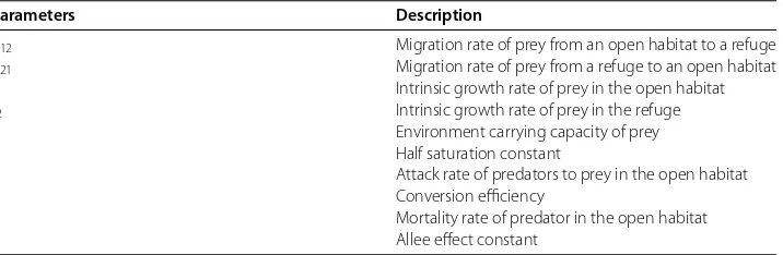
Parameters Description

C12 Migration rate of prey from an open habitat to a refuge

C21 Migration rate of prey from a refuge to an open habitat

r1 Intrinsic growth rate of prey in the open habitat

r2 Intrinsic growth rate of prey in the refuge

K Environment carrying capacity of prey

a Half saturation constant

b Attack rate of predators to prey in the open habitat

c Conversion eﬃciency

d Mortality rate of predator in the open habitat

A Allee eﬀect constant

responds only to the rate of prey killed per predator. Then we can set up the compartmen-tal model as follows:

⎧

Herex represents the number of prey in an open habitat,xrepresents the number of

prey in a refuge,yrepresents the number of predators in the open habitat. In this model, we consider the Allee eﬀect only in the equation ofx.

All the parameters are listed in Table . Ifbc≤d, predators can never grow, and then we assumebc>d.

It is a fact that the movement of prey is on a faster time scale than the growth and the death. According to the references [–], it is reasonable to consider two time scales for these parameters in the model. Letri=r˜i,b=b˜,d=d˜. Here is a small posi-tive parameter, which means that movements have a larger speed than that associated to growth and death processes. We obtain the fast system

⎧ patchi. We rewrite the fast system as follows:

⎧

(4)

and rd equations of (.), we obtain the following two-dimensional system:

In this model, the purpose is to study the impact of Allee eﬀect and the carrying capacity of prey. Here we only consider the particular caseC=C. Thenu∗=u∗= and system

Let the right-hand side of (.) equal to zero, we obtain

⎧

Thus, the equilibrium E= (, ) always exists. For the equilibria without predator, it

should satisfy the equation

Next we will study the dynamics at the slow time scale.

3 Dynamics of model (2.5) for the slow system

We ﬁrst calculate the Jacobian matrix for system (.)

J=

It is easy to calculate and obtain that

(5)

ThenEis a node point ifr˜<r˜and a saddle point ifr˜>r˜, and a saddle-node bifurcation

occurs atr˜=r˜.

ForE= (A(r_r˜_˜_–r˜), ) whenr˜<r˜.

JE=

a a

 a

,

where

a= ˜

r–r˜



 –A(r˜–r˜) Kr˜

,

a= –

Ab˜(r˜–r˜)

ar˜+ A(r˜–r˜)

< ,

a=

A(bc˜ –d˜)(r˜–r˜) –ad˜r˜

ar˜+A(r˜–r˜)

.

Note thatA≤Kandr˜–r˜<r˜, thena> . Hence,Eis an unstable source ifA>A

and is a saddle ifA<A, and a saddle-node bifurcation occurs atA=A.

ForE= (K, ) whenr˜<r˜.

JE=

a a

 a

,

where

a= ˜

r–r˜



 – Kr˜ A(r˜–r˜)

,

a=

K(bc˜ –d˜) –ad˜ a+K .

Note that A(r˜–r˜)

Kr˜ < , thena< . Hence,Eis an unstable source if K>K and is a saddle ifK<K, and a saddle-node bifurcation occurs atK=K.

ForE= (K, ) when r˜≥ ˜r. In this case a< . Hence,E is an unstable source if

K>Kand is a saddle ifK<K, and a saddle-node bifurcation occurs atK=K.

ForE∗= (x∗,y∗),

JE∗=

a a

a 

,

where

a=

˜ d c < ,

a=

(bc˜ –d˜)

abc˜ y

(6)

The characteristic equation ofJE∗is

The existence and stability of equilibria can be summered in the following Theorem ..

Theorem .

4 Hopf bifurcation analysis

In this section we study the dynamical behavior ofE∗ whenK=K. The characteristic

(7)

IfK=K,a= , and then the eigenvalues areλ,=±iωand the Hopf bifurcation will

occur. In this case,

ω=d˜

Now we calculate the ﬁrst Lyapunov coeﬃcient. Rewrite the coordinate ofEwhenK=

K:

Note that the slow system (.) is

⎧

Translate the origin of the coordinates to this equilibrium by the change of variables

⎧

This system can be represented as

(8)

where B=B(K), and the multilinear functionsCandDtake on the planar vectorsξ =

The eigenvalues ofBare

λ=

we can calculate that the eigenvectors are

q=

To achieve the necessary normalizationp,q = , we can take, for example,

(9)

Then we obtain

g=

p,C(q,q)=ad˜+ (bc˜ –d˜)d˜–dc˜ ωi,

g=

p,C(q,q¯)=ad˜,

g=

p,C(q,q,q¯)= ad˜.

The ﬁrst Lyapunov coeﬃcient is

l(K) = 

ωRe(igg+ωg)

=ωd˜



ω(ca+a)

< .

Therefore, a unique and stable limit cycle bifurcates from the equilibriumE∗via the Hopf bifurcation forK>K. This result is diﬀerent from the result in [].

Theorem . If K>K,a unique and stable limit cycle bifurcates from the equilibrium E∗

via the Hopf bifurcation.

5 Numerical simulation

Now we perform some simulations for the dynamics of the slow system (Figures -) and the original system (Figure ). According to some literature works, the values of param-eters are listed in Table . We choosea= ,b˜= .,c= .,d˜ = .. ThenK= ..

Some simulations are performed by Maple software (Figures -).

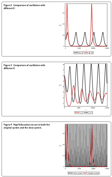
If we increase the environment carrying capacity of prey, Figure  shows that the period of predator oscillation is very long. In additional, a diﬀerent Allee eﬀect of prey in a refuge can lead to stable oscillation or stable endemic equilibrium state (Figure ).

At last we compare the dynamics of the original system with the slow system whenis small (Figure ). From Figure , we can see that the Hopf bifurcation occurs in both the original system and the slow system. The dynamics are similar, which also shows that the full dynamical system can be characterized by the dynamics on the slow manifold.

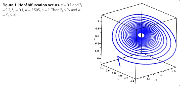
Figure 1 Hopf bifurcation occurs.= 0.1 and˜r1

= 0.2,˜r2= 0.1,K= 7.505,A= 1. Then˜r1>˜r2andK

(10)

Figure 2 Comparison of oscillation with differentK.

Figure 3 Comparison of oscillation with differentA.

Figure 4 Hopf bifurcation occurs in both the original system and the slow system.

6 Discussion

(11)

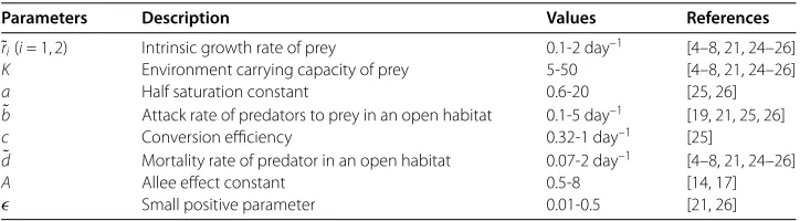
Table 2 The value of parameters

Parameters Description Values References

˜

ri(i= 1, 2) Intrinsic growth rate of prey 0.1-2 day–1 [4–8, 21, 24–26]

K Environment carrying capacity of prey 5-50 [4–8, 21, 24–26]

a Half saturation constant 0.6-20 [25, 26]

˜

b Attack rate of predators to prey in an open habitat 0.1-5 day–1 _{[19, 21, 25, 26]}

c Conversion eﬃciency 0.32-1 day–1 _[25]

˜

d Mortality rate of predator in an open habitat 0.07-2 day–1 _{[4–8, 21, 24–26]}

A Allee eﬀect constant 0.5-8 [14, 17]

Small positive parameter 0.01-0.5 [21, 26]

techniques, we separate the dynamics of the model into two time scales. Based on the-oretical analyses and numerical simulations (Figure ), we show that the full dynamical system can be characterized by the dynamics on the slow manifold in the long run. Then we analyze the stability of the system on the slow time scale. Our results show that when the carrying capacity for the prey populationKis greater than some valueK, the Hopf

bifurcation will occur. According to Figure , if the carrying capacity for the prey is en-sured abundant, the period will be longer and the amount of predators fluctuates greatly. In additional, reducing the Allee effect of prey will lead to stable periodical oscillation (Figure ), which is different from the result of [].

In nature, the growth rate of prey in a refuge should be less than that in an open habitat because of limitation of mating. According to Theorem ., this diﬀerence will lead to the equilibria without predator, and the equilibria without predator is unstable. This means that biological environment without predator is unstable in nature, which is in good agree-ment with some practical phenomena. For example [], Kaiba forest located in the north-ern margin of the Colorado Grand Canyon, Arizona. In , to protect the black tailed deer, people killed all the natural enemies of the forest. The number of deer in the forest began to increase sharply to ,, but by  the number reduced to ,. The rea-son is that the original ecosystem had been destroyed, more than its stability threshold, and thus became unstable.

Furthermore, when the carrying capacity of prey (K) is bigger than a critical value (K),

(12)

Competing interests

The authors declare that no competing interests exist.

Authors’ contributions

LQ established, analyzed and simulated the model and wrote the manuscript. LG proved the stability of the equilibria in Section 3. MX proved the Hopf bifurcation in Section 4. SS did some simulations in Section 5.

Acknowledgements

This research is supported by the National Natural Science Foundation of China (11401002), the Natural Science Foundation of Anhui Province (1208085QA15) and also by the Foundation for Young Talents in College of Anhui Province (2012SQRL021) and the National Scholarship Foundation of China. We would like to specially thank Professor Huaiping Zhu from York University of Canada for his guidance and help. We would like to thank anonymous reviewers for very helpful suggestions which improved greatly this manuscript.

Received: 20 April 2015 Accepted: 15 October 2015 References

1. Lidicker, WZ Jr: The Allee eﬀect: its history and future importance. Open Ecol. J.3, 71-82 (2010) 2. Stephens, PA, Sutherland, WJ, Freckleton, RP: What is the Allee eﬀect? Oikos87, 185-190 (1999) 3. Allee, WC: The Social Life of Animals, revised edn. Beacon Press, Boston, MA (1958)

4. Aviles, L: Causes and consequences of cooperation and permanent-sociality in spiders. In: Choe, J, Crespi, B (eds.) The Evolution of Social Behavior in Insects and Arachnids, pp. 476-497. Cambridge University Press, Cambridge (1997) 5. Clutton-Brock, TH, Gaynor, D, et al.: Predation, group size and mortality in a cooperative mongoose,Suricata suricatta.

J. Anim. Ecol.68, 672-683 (1999)

6. Courchamp, F, Clutton-Brock, TH, Grenfell, B: Multipack dynamics and the Allee eﬀect in the African wild dog,Lycaon pictus. Anim. Conserv.3, 277-285 (2000)

7. Heinsohn, RG: Cooperative enhancement of reproductive success in white-winged choughs. Evol. Ecol.6, 97-114 (1992)

8. Morris, DW: Measuring the Allee eﬀect: positive density dependence in small mammals. Ecology83, 14-20 (2002) 9. Morris, DW: How can we apply theories of habitat selection to wildlife conservation and management? Wildl. Res.30,

303-319 (2003)

10. Knight, TW, Morris, DW: How many habitats do landscapes contain? Ecology77, 1756-1764 (1996)

11. Holt, RD, Knight, TM, Barﬁeld, M: Allee eﬀects, immigration, and the evolution of species’ niches. Am. Nat.163, 253-262 (2004)

12. Jonzén, N, Wilcox, C, Possingham, HP: Habitat selection and population regulation in temporally ﬂuctuating environments. Am. Nat.164, 103-114 (2004)

13. Berezovskaya, FS, Song, BJ, Castillo-Chavez, C: Role of prey dispersal and refuges on predator-prey dynamics. SIAM J. Appl. Math.70, 1821-1839 (2010)

14. Boukal, DS, Sabelis, MW, Berec, L: How predator functional responses and Allee eﬀects in prey aﬀect the paradox of enrichment and population collapses. Theor. Popul. Biol.72, 136-147 (2007)

15. Kühnová, J, Pˇribylová, L: A predator-prey model with Allee eﬀect and fast strategy evolution dynamics of predators using hawk and dove tactics. Tara Mt. Math. Publ.50, 13-24 (2011)

16. Wang, JF, Shi, JP, Wei, JJ: Predator-prey system with strong Allee eﬀect in prey. J. Math. Biol.62, 291-331 (2011) 17. Zhou, SR, Liu, YF, Wang, G: The stability of predator-prey systems subject to the Allee eﬀects. Theor. Popul. Biol.67,

23-31 (2005)

18. Zu, J, Mimura, M: The impact of Allee eﬀect on a predator-prey system with Holling type II functional response. Appl. Math. Comput.217, 3542-3556 (2010)

19. Auger, P, de la Parra, RB, Morand, S, Sánchez, E: A predator-prey model with predators using hawk and dove tactics. Math. Biosci.177, 185-200 (2002)

20. Arditi, R, Ginzburg, LR: Coupling in predator-prey dynamics: ratio-dependence. J. Theor. Biol.139, 311-326 (1989) 21. Auger, P, de la Parra, RB, Poggiale, JC, Sánchez, E, Nguyen-Huu, T: Aggregation of variable and application to

population dynamics. In: Structured Population Models in Biology and Epidemiology, pp. 209-263. Springer, Berlin (2008)

22. Feng, ZL, Yi, YF, Zhu, HP: Fast and slow dynamics of malaria and the s-gene frequency. J. Dyn. Diﬀer. Equ.16, 869-895 (2004)

23. Fenichel, N: Geometric singular perturbation theory for ordinary differential equations. J. Differ. Equ.31, 53-98 (1979) 24. Doanh, N, Tri, N, Pierre, A: Effects of refuges and density dependent dispersal on interspecific competition dynamics.

Int. J. Bifurc. Chaos22, 1250029 (2012). doi:10.1142/S0218127412500290

25. Jana, S, Chakraborty, M, Chakraborty, K, Kar, TK: Global stability and bifurcation of time delayed prey-predator system incorporating prey refuge. Math. Comput. Simul.85, 57-77 (2012)

26. Poggiale, JC, Michalski, J, Arditi, R: Emergence of donor control in patchy predator-prey systems. Bull. Math. Biol.60, 1149-1166 (1998)

27. A story about ecological balance. http://zhidao.baidu.com/link?url=3gbLqtuJH-B5yKqpklY5a3g22BtROUo56auLZoc H3qaD0feDw3DB-OoSk0ngJrIQVyMmdOkry2CJM4-_gjnsSa