R E S E A R C H
Open Access
Generation of 2D correlated random
shadowing based on the deterministic
MR-FDPF model
Meiling Luo
*, Guillaume Villemaud and Jean-Marie Gorce
Abstract
In modern mobile telecommunications, shadow fading has to be modeled by a two-dimensional (2D) correlated random variable since shadow fading may present both cross-correlation and spatial correlation due to the presence of similar obstacles during the propagation. In this paper, 2D correlated random shadowing is generated based on the multi-resolution frequency domain ParFlow (MR-FDPF) model. The MR-FDPF model is a 2D deterministic radio propagation model, so a 2D deterministic shadowing can be firstly extracted from it. Then, a 2D correlated random shadowing can be generated by considering the extracted 2D deterministic shadowing to be a realization of it. Moreover, based on the generated 2D correlated random shadowing, a complete 2D semi-deterministic path loss model can be proposed. The proposed methodology of this paper can be implemented into system-level simulators where it will be very useful due to its ability to generate realistic shadow fading.
Keywords: Correlated shadowing; Indoor radio propagation; Large scale propagation; Semi-deterministic model; Small scale fading
1 Introduction
The exponential growth of mobile traffic in the past two decades has set a formidable challenge to the wireless system capacity, thus the heterogeneous networks were proposed to offload a part of traffic to small cells, e.g., Femtocells. Before actual deployments, the design of such small cell networks and also WiFi networks is usually through network planning and optimization tools. The efficiency of the network planning and optimization tools depends strongly on the accuracy of the used radio prop-agation models or channel models. Hence, a careful selec-tion of radio propagaselec-tion models or channel models is necessary for an efficient and valid network design.
This paper focuses mainly on the shadow fading model-ing. Many channel measurements have confirmed that the probability density function (PDF) of the shadow fading in logarithmic scale can be approximated by a Gaussian (nor-mal) distribution with zero mean and certain standard deviation [1, 2]. Then in linear scale, this is a lognormal distribution. For this reason, shadow fading is also usually
*Correspondence: [email protected]
Université de Lyon, INRIA, INSA-Lyon, CITI, F-69621 Villeurbanne, France
called the lognormal fading. However, measurements have also shown that shadow fading presents both the cross-correlation and the spatial correlation [3–7]. Thus, a totally independent one-dimensional lognormal shadow fading fails to well represent the shadow fading for real systems and a two-dimensional (2D) shadow fading model is preferred. Extensive research has been conducted on how to accurately model the shadow fading, e.g., how to model the cross-correlation and spatial correlation existing in the realistic shadow fading [3, 4, 7] and how to include them into the 2D shadow fading models [8–12]. For instance, in [3], Saunders et al. proposes a cross-correlation model for the shadow fading. In [7], Gudmundson proposes a spatial correlation model for the shadow fading in mobile radio channels by measurement data fitting. This model now is widely accepted by many researchers and it is almost regarded as a standard spa-tial correlation model to be included into the proposed 2D shadow fading models [8–12]. However, Gudmundson’s spatial correlation model is proposed mainly for large to moderate cell sizes. For small cell sizes, e.g., Femtocells, it suffers from a low level of accuracy.
The main concern of this paper is the shadow fading modeling of small cells. Since the commonly used correla-tion models do not work very well for small cells, we pro-pose in this paper to calculate the cross-correlation and spatial correlation from the site-specific multi-resolution frequency domain ParFlow (MR-FDPF) model [13–15], i.e., no need to make any assumptions about the cross-correlation and spatial cross-correlation models. Then, the calculated site-specific cross-correlation and spatial cor-relation are included into the proposed 2D correlated random shadowing model by applying the method of Fraile et al. in [8]. The MR-FDPF model is a deterministic site-specific radio propagation model, so it possesses the property of a high level of accuracy. For the same reason, the MR-FDPF model also suffers from a high computa-tional load. Thus, the MR-FDPF model is normally limited to simulate the small cell scenarios, such as the indoor radio propagation scenarios.
Based on the generated 2D correlated random shadow fading, a complete 2D semi-deterministic path loss model can be proposed. The reason why we propose a 2D semi-deterministic path loss model is that the high level of accuracy of a pure deterministic model can not guarantee a high level of realism for real systems. As stated above, as a deterministic model, the MR-FDPF model possesses a high level of accuracy if the propagation scenario is well modeled firstly. However, the most difficult thing is how to model the propagation scenario perfectly. In reality, modeling the propagation scenario with 100 % accuracy is almost an impossible task. For instance, sometimes there can be some moving people or moving objects present in real propagation scenarios. But these moving people or moving objects are difficult to be modeled in simulations. Besides, the positions of walls and furniture in the prop-agation scenarios cannot be drawn with 100 % accuracy in the simulations. However, the minor inaccuracy of the scenario modeling may result in large prediction error due to the change of directions of multipath signals which are very crucial for the final multipath signal addition. There-fore, the high level of accuracy of deterministic models
depends strongly on the accuracy of the scenario model-ing. Since the accuracy of the scenario modeling cannot be always guaranteed first, the high level of accuracy of deterministic models does not mean that they are realis-tic. In this paper, we propose the 2D semi-deterministic path loss model aiming at improving the level of realism. In this model, the mean path loss is modeled determinis-tically, whereas the shadow fading and small-scale fading are modeled statistically.
The rest of the paper is organized as follows. Section 2 gives an introduction of the MR-FDPF model including its calibration and accuracy analysis. Then in Section 3, we discuss first how to extract the 2D deterministic shad-owing from the MR-FDPF model. Based on the extracted 2D deterministic shadowing, the 2D correlated random shadowing can be generated. In Section 4, a complete 2D semi-deterministic path loss model is proposed, followed by the simulation and experimental evaluation in Section 5. Finally, conclusion is drawn in Section 6.
2 The MR-FDPF model
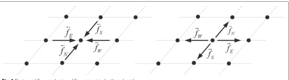
The MR-FDPF model is a deterministic radio propagation model. In this model, the simulated scenarios should be firstly discretized into a 2D grid-based structure and then it is assumed that the electric field corresponding to each grid point can be divided into four directive flows: the west, east, north, and south flow as shown in Fig. 1. The inward flows bring energy into the grid while the outward flows radiate energy out. In the conventional ParFlow model [16–18] which is a time-domain solver, the inward flows and outward flows are updated alternately according to a local scattering equation determined by the property of material of the grid. After a sufficient number of itera-tions in time domain, these flows will finally reach a steady state and then the steady-state radio coverage can be com-puted. However, in the MR-FDPF model, the steady-state radio coverage problem is solved directly in the frequency domain. Moreover, in the frequency domain, the MR-FDPF model introduces a multi-resolution structure and a preprocessing phase to reduce the computational load.
A calibration process is usually considered to be imper-ative for any radio wave propagation model since the properties of materials in the simulated scenarios are never exactly known. For the MR-FDPF model, the effect of materials in the simulated scenarios to the electromag-netic waves depends on two parameters: the refraction index nr and the normalized absorption coefficient ar. Hence, the two parameters of the materials in the sim-ulated scenarios need to be calibrated in the calibration process. It is noted that the absorption coefficient of the air aair plays an important role in the MR-FDPF model since it modifies the 2D free space path loss model from PL(d)∝dtoPL(d)∝d·a−aird/r, while a realistic 3D free space path loss model isPL(d)∝d2, wheredis the Tx-Rx (transmitter and receiver) separation distance andris the discretization space step. The approximation between PL(d)∝d·aair−d/randPL(d)∝d2can be effective over a finite range after an appropriate choice of theaair[19].
The calibration process of the MR-FDPF model is imple-mented in two steps. The first step is to estimate the constant offset as follows measurements and simulations, respectively, andKis the total number of samples. A constant offset always exists because of the numerical sources used in the MR-FDPF model, compared to the real transmitters in reality. The second step of the calibration process is to estimate the normalized absorption coefficient of airaair, the refraction index and normalized absorption coefficient of materials (nmat,amat)by minimizing the cost-functionQdefined by the root mean square error (RMSE) between measure-ments and predictions
are the mean powers from predictions. The minimization process is based on the direct search algorithm “DIRECT” by Jones et al. in [20]. A more detailed description about the calibration process of the MR-FDPF model can be found in [21].
In the following, we calibrate the MR-FDPF model with two sets of measurement data so that we can observe which level of accuracy the MR-FDPF model can normally achieve. The set of channel measurement conducted at Stanford University has been chosen, and specifically it corresponds to the “I2I stationary” scenario measurement therein [22].
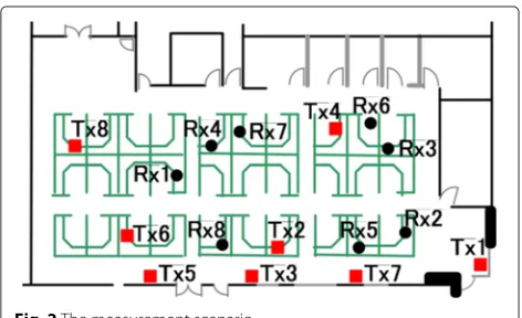
The scenario was a typical 16×34 m office environment made of 30 cubicles and 7 small separated rooms. Eight transmitters and 8 receivers were distributed in the office as illustrated in Fig. 2. All of them were equipped with omnidirectional antennas and were fixed in their locations during the measurement. Four materials were mainly used in the office, i.e.,concretefor the main walls,plasterfor the internal walls,glassfor the external glass wall, andwood for the cubicles located in the central part of the office.
In this channel measurement, 8 × 8 multiple-input multiple-output (MIMO) channels at a center frequency of 2.45 GHz were measured simultaneously with a RUSK MEDAV channel sounder [23]. For the measurement data, totally 120 time blocks covering a time duration of 32 s and 220 frequency bins covering a bandwidth of 70 MHz were recorded.
In the following, we calibrate the MR-FDPF model in two cases. The first case is to calibrate the MR-FDPF model with all the available measurement data, while the second case is to calibrate it with only a part of the avail-able measurement data. Intuitively, the prediction per-formance of the MR-FDPF model calibrated with all the measurement data should be better than that calibrated with only a part of the measurement data since more measurement data are used.
2.1 Calibration with the measurement data from the links between all Txs and all Rxs
This calibration is performed with the measurement data from all the 64 links, i.e., the links between all the 8 Txs and all the 8 Rxs. The measurement data used to perform the calibration are taken only from the center frequency of 2.45 GHz but are averaged along the time axis, i.e., averaged over the 120 time blocks.
The parameter values of materials obtained from the calibration process are listed in Table 1.
Then, these parameter values are configured to run the MR-FDPF simulation at 2.45 GHz with 0 dBm transmit power. The simulation step is 2 cm. The radio coverage
Table 1Parameter values of materials optimized from calibration A
nmat amat
Air 1.0 0.9999335
Absorbant 1.0 0.96879673
Wood 4.002058 0.9999999
Plaster 1.5 0.9999999
Concrete 5.4 0.9999999
Glass 2.1042523 0.9999999
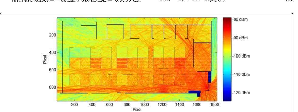
map of Tx1 simulated with the MR-FDPF model is shown in Fig. 3 as an example.
The obtained offset and the RMSE computed from the 64 links compared to the measurement data are: offset= −60.3912 dB; RMSE=4.6618 dB;
2.2 Calibration with the measurement data from the links between only Tx1 and all Rxs
This calibration is performed with the measurement data from 8 links, i.e., the links between the Tx1 and all the 8 Rxs. The same as above, the measurement data used to perform the calibration are taken only from the center fre-quency of 2.45 GHz but are averaged over the 120 time blocks.
The obtained parameter values of materials from the calibration process are listed in Table 2.
Similarly, these parameters are also configured to run the MR-FDPF simulations at 2.45 GHz. Thus, we can com-pute the offset and the RMSE between the simulation and measurement as follows:
• The offset and the RMSE computed only from the 8 links are: offset= −62.1031dB; RMSE= 4.3858dB; • The offset and the RMSE computed from all the 64
links are: offset= −60.2297dB; RMSE= 8.5705dB;
Comparing the two RMSEs computed both from the 64 links in the above two different cases A and B, it is obvi-ous that we obtain a smaller RMSE when all the simulated points are calibrated with the measurement data than only a part of them are calibrated, which is consistent with our intuition.
3 Generation of the 2D correlated random
shadowing
In this section, we talk about how to generate the 2D correlated random shadowing based on the MR-FDPF model.
As is known, when expressed in dB, the instantaneous path loss can be expressed as the sum of the mean path loss, the shadow fading, and the small-scale fading as follows
PL(d)=L(d)+Xσ+F (4)
where PL(d),L(d), Xσ, and F denote the instantaneous path loss, the mean path loss, the shadow fading, and the small-scale fading, respectively. The mean path lossL(d) and the shadow fading Xσ characterize the signal varia-tions over large distances, so they are usually called the large-scale propagation characteristics. On the contrary, theFis called the small-scale fading since it characterizes the rapid signal fluctuations over very short distances, e.g., over several wavelengths.
3.1 Extraction of the 2D deterministic shadowing from the MR-FDPF model
In (4), the termL(d)is considered to be deterministic and thus it can be described in a deterministic manner. Typ-ically, the mean path loss L(d) is log dependent on the Tx-Rx separation distancedas follows
L(d)=L0+10n·log10(d) (5)
Table 2Parameter values of materials optimized from calibration B
nmat amat
Air 1.0 0.9999997
Absorbant 1.0 0.96879673
Wood 2.3888888 0.9999999
Plaster 1.5 0.9999999
Concrete 5.4 0.9999999
Glass 2.0438957 0.9999999
whereL0is a constant which accounts for system losses andnis the path loss exponent depending on the specific propagation environment. For instance,n=2 for the free space propagation. The mean path loss is the main factor which determines the coverage area of a transmitter.
The shadow fading Xσ is normally a Gaussian dis-tributed random variable (in dB) with zero mean and standard deviationσX[2].
At last, the small-scale fadingFin linear scale is typically either a Rayleigh random variable (for NLOS propaga-tion) or a Rician random variable (for LOS propagapropaga-tion). However, for real propagation scenarios, it is sometimes very difficult to tell whether it is a pure NLOS or a LOS propagation. Thus, here we would like to model the small-scale fading by the Nakagami-m fading which includes the Rayleigh fading and Rice fading as special cases [24].
Moreover, recently the Nakagami-mfading has received more and more attention because it gives the best fit to many measurement data, such as land-mobile and indoor-mobile multipath propagation [2, 25].
As stated above, the small-scale fading represents the rapid signal fluctuations over short distances, so they can be removed by averaging over local areas. After remov-ing the small-scale fadremov-ing, we obtain the local mean path loss. The local mean path loss includes the mean path loss and the shadow fading as shown in Fig. 4. Since we already know that the mean path loss is log dependent on the Tx-Rx separation distancedaccording to (5), we can obtain the mean path loss by using the Matlab curve fitting tool. And finally, the shadow fading can be easily obtained by subtracting the mean path loss from the local mean path loss. The above procedures can be applied to the simu-lation results of the MR-FDPF model in order to obtain the large-scale propagation characteristics, which is one of our previous works published in [26].
Since the simulation results provided by the MR-FDPF model are deterministic, the extracted shadow fading from the MR-FDPF model is also deterministic.
3.2 Generation of the 2D correlated random shadowing
Since the MR-FDPF model is a 2D deterministic radio propagation model and it takes the specific propagation environment into account, the extracted shadow fading from the MR-FDPF model is a 2D correlated deterministic
shadow fading. However, for real systems, shadow fading should only be modeled statistically due to the difficulty in modeling the randomly moving people and moving objects present in real environments. Thus, a random shadow fading is considered to be more realistic and more accurate than a deterministic shadow fading. In fact, in modern mobile telecommunications, shadow fading has to be modeled to be 2D correlated random shadowing since shadow fading may present both cross-correlation and spatial correlation due to the presence of similar obstacles during the propagation. For instance, nearby receivers are probable to experience very similar shadow fadings, i.e., their shadow fadings are correlated.
Now, we detail how to generate the 2D correlated ran-dom shadowing model based on the 2D correlated deter-ministic shadow fading provided by the MR-FDPF model. It is based on the method of Fraile et al. in [8]. Assume that there are totallyItransmitters in the simulated sce-nario. The MR-FDPF model can provide a deterministic shadow fading map for each of these transmitters, e.g., shadow fading map i for transmitteri. For each point (x,y)(i.e., where the virtual receiver is) in the simulated scenario, the shadow fading experienced by signals trans-mitted fromItransmitters can be modeled byI+1 inde-pendent Gaussian random variables{G0,G1· · ·GI}which have zero mean and the same standard deviationσX. To make sure that the generated shadow fading exhibits the same cross-correlation as presented in real systems, the shadow fading can be generated as follows:
Xσij= √ρij·G0+
1−ρij·Gi (6)
where Xσij is the generated shadow fading for transmit-teriwhile taking into account its cross-correlation from transmitterj, withi,j∈ {1, 2· · ·I}.
From the above, it is easy to know that
EXσij =0 (7)
SXσij =σX (8)
whereE(·)andS(·)denote the expectation and the stan-dard deviation. Thus, it guarantees that the generated shadow fading is still a Gaussian random variable with zero mean and standard deviation equal to σX. Mean-while, it also guarantees that the cross-correlation of shadow fadings between any pair of transmittersi,jis equal to
Thus, in this approach, the common component G0 is used to model the receiver-position-dependent cross-correlation of shadow fadings from different transmitters. Since the same procedure above can be repeated at each point(x,y)in the simulated scenario to generate the correlated shadow fading, the generated 2D cross-correlated shadow fading map can be rewritten as:
Xσij(x,y)=
Although the above generated 2D shadow fadings are cross-correlated, there is not any spatial correlation inside (the correlation of the shadow fadings is zero when their positions are different). In order to generate the spatial correlation, a 2D filter can be applied to the 2D cross-correlated shadow fading map.
The impulse response of the 2D filter is denoted by h(x,y). The input of the 2D filter is supposed to be the above generated 2D cross-correlated shadow fading map, i.e., a(x,y) = Xijσ(x,y). The output b(x,y) is the expected shadow fading map which presents both the cross-correlation and the spatial correlation. As we know, if the impulse responseh(x,y)of the 2D filter is known, the outputb(x,y)can be easily obtained by a 2D convo-lution between the inputa(x,y)and the impulse response h(x,y). Thus, the main task we should do here is to try to obtain the impulse responseh(x,y)of the 2D filter.
According to the theory of random processes and linear systems, the power spectral density ofb(x,y)is related to the power spectral density ofa(x,y)according to
Sbb(fx,fy)=Saa(fx,fy)·H(fx,fy)2 (11)
whereSbb(fx,fy),Saa(fx,fy)are the power spectral density of b(x,y) and that ofa(x,y), respectively.H(fx,fy) is the system transfer function of the 2D filter. Since the input a(x,y)=Xσij(x,y)is a white shadow fading map, its auto-correlation functionRaa(x,y)is non-zero only at the position(0, 0). Thus, its power spectral density is flat
Saa
After a simple mathematical derivation, we can find σ2
a = σX2. Therefore, the system transfer function can be obtained by obtained by performing a 2D inverse Fourier transform to the system transfer function.
Rbb(x,y). Here, the deterministic shadow fading map provided by the MR-FDPF model is considered to be one realization of the random process ofb(x,y).
4 A complete 2D semi-deterministic path loss
model
Based on the generated 2D correlated random shadowing above, a complete 2D semi-deterministic path loss model can be structured as follows
PLij(x,y)=L(d)+b(x,y)+F(x,y) (14)
where PLij(x,y) is the 2D path loss at position(x,y) of the transmitter i while taking into account the cross-correlation of the shadow fading from the transmitter j,
and d =
(x−xi)2+(y−yi)2 is the distance to the transmitteriat position of(xi,yi),L(d)is the mean path loss,b(x,y)is the generated 2D correlated random shad-owing, and F(x,y) is the small-scale fading which can be determined by the m parameter of the Nakagami-m fading.
Specifically, the above mean path loss L(d), shadow fading b(x,y), and the small-scale fadingF(x,y) can be determined as follows:
• The mean path lossL(d)is deterministic and it can be determined from the MR-FDPF model as detailed in Section 3.1.
• The shadow fadingb(x,y)can be generated as detailed in Section 3.2 which is a 2D correlated random shadowing.
• The small-scale fadingF(x,y)is a Nakagami-m distributed random variable in linear scale. Since here F(x,y)is in dB, a variable transformation
F=10·log10α2is needed (αis Nakagami-m
distributed). Therefore, the probability density function ofF is finally
PF(F) =
wherem is the estimated m parameter of the Nakagami-m fading and=E10F/ 10.
This 2D semi-deterministic path loss model is com-plete because it takes into account both the large-scale fading and the small-scale fading. Moreover, it also takes into account the cross-correlation and the spatial correla-tion of the shadow fading. We call it a semi-deterministic model because it is mainly based on the deterministic MR-FDPF model, but it also introduces a random part to model the randomness of realistic radio channels.
5 Simulation and experimental evaluation
In order to verify the proposed approach, we still choose the Stanford’s office scenario to perform the MR-FDPF simulation which has been detailed in Section 2. The MR-FDPF simulation is performed with the material parame-ter values listed in Table 1. It is simulated at the frequency of 2.45 GHz and with the transmit power of 0 dBm. The simulation step is 2 cm. An example of the radio cover-age map simulated with the MR-FDPF model has been presented in Fig. 3.
As described previously, the small-scale fading can be modeled by the Nakagami-mfading and it can be removed by doing averaging over local areas. Moreover, the sever-ity of the small-scale fading can be indicated by the m parameter of the Nakagami-m fading which can be efficiently estimated by the Greenwood’s method [27].
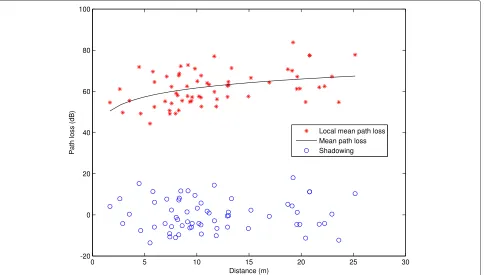
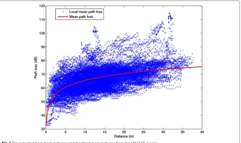
Fig. 6The extracted local mean path loss and the fitted mean path loss from the MR-FDPF model
Figure 5 shows the estimatedmparameter map which is obtained by doing exactly the same processes as in our previous work [28], e.g., each m parameter is obtained over a local area with dimensions 23×23 pixels and its estimation performance has been verified by conducting the Kolmogorov-Smirnov goodness of fit test. For more details, readers can refer to [28].
After averaging out the small-scale fading over local areas, we obtain the local mean path loss from the MR-FDPF simulation as shown in Fig. 6 by the blue crosses. In this figure, the local mean path loss is obtained from all the
8 transmitters and all the local areas in the scenario. Thus, by using the Matlab curve fitting tool, we obtain the fitted mean path loss for the whole scenario from simulation as shown in Fig. 6. It is
Lsim(d)=49.05+10×1.653·log10(d) (16)
On the other hand, the fitted mean path loss from the Standord’s channel measurement is [26]
Lmeas(d)=47.25+10×1.442·log10(d) (17)
Comparing them two, we can see that the obtained L0 and path loss exponentnfrom the simulation and
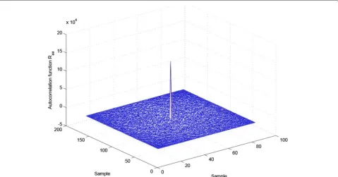
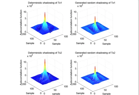
Fig. 8The autocorrelation function of the extracted 2D deterministic shadowing from the MR-FDPF model
surement are comparable, which demonstrates that the MR-FDPF simulation result is accurate.
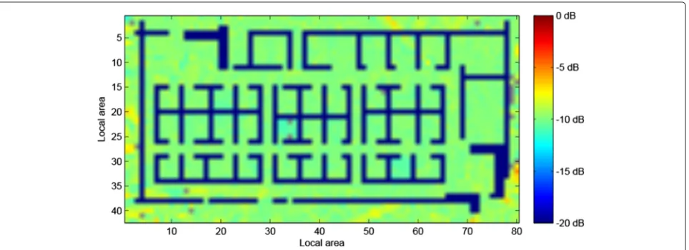
When we have both the local mean path loss and the mean path loss, we can easily obtain the deterministic shad-owing from the MR-FDPF model by just subtracting the
mean path loss from the local mean path loss. Figure 7 shows the 2D deterministic shadowing from the MR-FDPF model. From this figure, we can see that the 2D deterministic shadowing from the MR-FDPF model is correlated. This is reasonable since the MR-FDPF model is
Fig. 10The generated 2D random shadowing with cross-correlation
a site-specific model, i.e., it takes into account for instance, the walls, the furniture, and so on in the propagation environments.
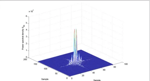
Although it is obvious in Fig. 7 that the 2D determinis-tic shadowing from the MR-FDPF model is correlated, we want to know how much it is correlated. Thus, we check the 2D autocorrelation function of the extracted deter-ministic shadowing from the MR-FDPF model which is presented in Fig. 8. Since the autocorrelation function and the power spectral density are a Fourier transform pair, we can easily obtain the power spectral density by applying
a 2D Fourier transform to the autocorrelation function as shown in Fig. 9.
Now in the following part, the generated 2D ran-dom shadowing results are presented. In Fig. 10, we present the generated 2D random shadowing of Tx1 which has taken into account the cross-correlation from Tx2 as an example. It is generated according to (10). We can also check its autocorrelation function as shown in Fig. 11. As is seen, since the generated 2D random shadowing here has only taken into account the cross-correlation but not yet the spatial cross-correlation, the
Fig. 12The generated 2D random shadowing with both the cross-correlation and the spatial correlation
correlation function is almost non-zero only at the center.
The generated 2D random shadowing with both the cross-correlation and the spatial correlation is presented in Fig. 12. From this figure, we can easily see that there
is a spatial correlation inside the generated 2D random shadowing. Although it is obvious that there exists a spatial correlation in Fig. 12, it tells nothing about how the spatial correlation is, especially how the spatial cor-relation matches that of the deterministic shadowing
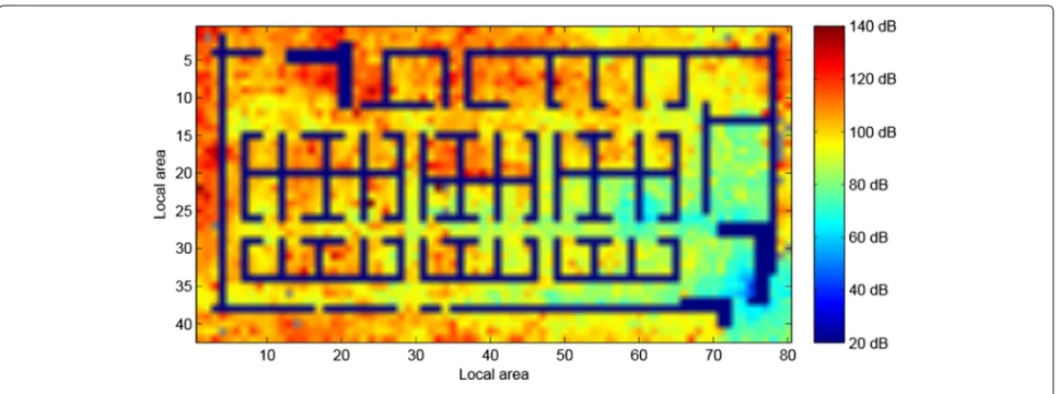
Fig. 14The generated 2D semi-deterministic path loss for Tx1
extracted from the MR-FDPF model. Hence, we com-pare the autocorrelation function of the generated 2D correlated random shadowing to that of the determin-istic shadowing extracted from the MR-FDPF model in Fig. 13. From this figure, we can see that although the autocorrelation functions do not match each other exactly, they show some similarities.
At the end of this section, we present the result of the generated 2D semi-deterministic path loss. Here in Fig. 14, we show the generated 2D semi-deterministic path loss for Tx1 as an example. It is obtained according to (14), whereL(d) = 49.05+10×1.653·log10(d),Xσij(x,y)is the above generated 2D correlated random shadowing and F(x,y)is generated according to (15).
6 Conclusions
In this paper, the generation of a realistic shadow fading for small cells is mainly addressed. Since a one-dimensional lognormal shadow fading cannot well rep-resent the shadow fading for real systems, for instance, it can not model the cross-correlation and the spatial correlation presented in the realistic shadow fading, a 2D correlated random shadowing is generated in this paper. It is generated based on the extracted deter-ministic shadowing from the MR-FDPF model which is considered to be one realization of the 2D corre-lated random shadowing. Since the deterministic MR-FDPF model is a site-specific model, the extracted deterministic shadowing from it is efficient, which has been also been verified by comparison to the channel measurement.
Based on the generated 2D correlated random shadowing, a complete 2D semi-deterministic path loss model is also pro-posed at the end. This 2D path loss model is complete because it takes into account not only the large-scale
fading and the small-scale fading but also the cross-correlation and the spatial cross-correlation of the shadow fading.
The methodology proposed in this paper can be implemented into system-level simulators and it will be very useful for them due to its ability to generate realistic shadow fading.
Competing interests
The authors declare that they have no competing interests.
Acknowledgements
This work is funded by the FP7 IPLAN Project.
Received: 10 December 2014 Accepted: 10 August 2015
References
1. WC Lee,Mobile Communications Engineering. (McGraw-Hill Professional, New York, 1982)
2. MK Simon, MS Alouini,Digital Communication over Fading Channels86. (Wiley-IEEE Press, Hoboken, 2004)
3. SR Saunders, A Aragón-Zavala,Antennas and Propagation for Wireless Communication Systems. (Wiley, Hoboken, 2007)
4. V Graziano, Propagation correlations at 900 MHz. IEEE Trans. Veh. Technol. 27(4), 182–189 (1978)
5. J Van Rees, Cochannel measurements for interference limited small-cell planning. AEU. Archiv für Elektronik und Übertragungstechnik.41(5), 318–320 (1987)
6. AJ Viterbi, AM Viterbi, E Zehavi, Other-cell interference in cellular power-controlled cdma. IEEE Trans. Commun.42(234), 1501–1504 (1994) 7. M Gudmundson, Correlation model for shadow fading in mobile radio
systems. Electron. Lett.27(23), 2145–2146 (1991)
8. R Fraile, JF Monserrat, J Gozálvez, N Cardona, Mobile radio bi-dimensional large-scale fading modelling with site-to-site cross-correlation. Eur. Trans. Telecommun.19(1), 101–106 (2008)
9. JF Monserrat, R Fraile, D Calabuig, N Cardona. Complete shadowing modeling and its effect on system level performance evaluation, (2008), pp. 294–298. http://ieeexplore.ieee.org/xpl/login.jsp?tp=&arnumber= 4525629&url=http%3A%2F%2Fieeexplore.ieee.org%2Fxpls%2Fabs_all.jsp %3Farnumber%3D4525629
http://ieeexplore.ieee.org/xpl/login.jsp?tp=&arnumber=1651489&url= http%3A%2F%2Fieeexplore.ieee.org%2Fxpls%2Fabs_all.jsp%3Farnumber %3D1651489
11. I Forkel, M Schinnenburg, M Ang, Generation of two-dimensional correlated shadowing for mobile radio network simulation. WPMC, sep. 21, 43 (2004)
12. X Cai, GB Giannakis, A two-dimensional channel simulation model for shadowing processes. IEEE Trans. Veh. Technol.52(6), 1558–1567 (2003) 13. J-M Gorce, K Jaffres-Runser, G de la Roche, Deterministic approach for fast
simulations of indoor radio wave propagation. IEEE Trans. Antennas Propag.55(3), 938–948 (2007). doi:10.1109/TAP.2007.891811 14. D Umansky, JM Gorce, M Luo, G De La Roche, G Villemaud,
Computationally efficient MR-FDPF and MR-FDTLM methods for multifrequency simulations. IEEE Trans. Antennas Propag.61(3), 1309–1320 (2012)
15. K Runser, J-M Gorce, in61st IEEE Vehicular Technology Conference. Assessment of a new indoor propagation prediction method based on a multi-resolution algorithm (Stockholm, Sweden, 2005).
doi:10.1109/VETECS.2005.1543244, http://ieeexplore.ieee.org/xpl/login. jsp?tp=&arnumber=1543244&url=http%3A%2F%2Fieeexplore.ieee.org %2Fiel5%2F10360%2F32958%2F01543244.pdf%3Farnumber %3D1543244
16. B Chopard, P Luthi, J-F Wagen, inThe Ninth IEEE International Symposium on Personal, Indoor and Mobile Radio Communications. Multi-cell coverage predictions: a massively parallel approach based on the parflow method, vol. 1, (1998), pp. 60–64. doi:10.1109/PIMRC.1998.733511, http:// ieeexplore.ieee.org/xpl/login.jsp?tp=&arnumber=733511&url=http%3A %2F%2Fieeexplore.ieee.org%2Fxpls%2Fabs_all.jsp%3Farnumber %3D733511
17. B Chopard, PO Luthi, J-F Wagen, Lattice Boltzmann method for wave propagation in urban microcells. IEE Proc. Microwaves Antennas Propag. 144(4), 251–255 (1997). doi:10.1049/ip-map:19971197
18. PO Luthi (1998). http://cuiwww.unige.ch/~luthi/a.pdf
19. G de la Roche, K Jaffres-Runser, J-M Gorce, On predicting in-building WiFi coverage with a fast discrete approach. Int. J. Mob. Netw. Des. Innov.2(1), 3–12 (2007)
20. DR Jones, CD Perttunen, BE Stuckman, Lipschitzian optimization without the Lipschitz constant. J. Optim. Theory Appl.79(1), 157–181 (1993) 21. GDL Roche, K Jaffrès-Runser, J-M Gorce, G Villemaud, The Adaptive
Multi-Resolution Frequency-Domain ParFlow AR-MDPF method for 2D Indoor radio wave propagation simulation. part II : Calibration and experimental assessment. Tech. Rep. (2005). http://raweb.inria.fr/ rapportsactivite/RA2006/ares/bibliography.html. INRIA, Nov 2006 22. N Czink, B Bandemer, G Vazquez-Vilar, A Paulraj, L Jalloul (2008). http://
www.gonzalo-vazquez-vilar.eu/files/08cost-TD(06)620-compressedimg. pdf
23. RUSK MEDAV channel sounders (2008). http://www.channelsounder.de 24. M Nakagami, inStatistical Method in Radio Wave Propagation, ed. by WC Hoffman. The m-distribution-A general formula of intensity distribution of rapid fading (Pergamon Oxford UK, 1960), pp. 3–36
25. A Sheikh, M Abdi, M Handforth, in43rd IEEE Vehicular Technology Conference. Indoor mobile radio channel at 946 MHz: measurements and modeling (Secaucus, NJ, USA, 1993). http://ieeexplore.ieee.org/xpl/ articleDetails.jsp?arnumber=507014
26. M Luo, N Lebedev, G Villemaud, G De La Roche, J Zhang, JM Gorce, in6th European Conference on Antennas and Propagation (EUCAP). On predicting large scale fading characteristics with the MR-FDPF method (Prague, Czech Republic, 2012). http://ieeexplore.ieee.org/xpl/login.jsp?tp= &arnumber=6206282&url=http%3A%2F%2Fieeexplore.ieee.org%2Fxpls %2Fabs_all.jsp%3Farnumber%3D6206282
27. JA Greenwood, D Durand, Aids for fitting the gamma distribution by maximum likelihood. Technometrics.2(1), 55–65 (1960)
28. M Luo, G Villemaud, J Weng, J-M Gorce, J Zhang, inIEEE Wireless Communications and Networking Conference (WCNC 2013), Shanghai, China, April. Realistic prediction of BER and AMC Woth MRC diversity for indoor wireless transmissions, (2013). http://ieeexplore.ieee.org/xpl/login. jsp?tp=&arnumber=6555227&url=http%3A%2F%2Fieeexplore.ieee.org %2Fiel7%2F6548699%2F6554525%2F06555227.pdf%3Farnumber %3D6555227
Submit your manuscript to a
journal and benefi t from:
7 Convenient online submission 7 Rigorous peer review
7 Immediate publication on acceptance 7 Open access: articles freely available online 7 High visibility within the fi eld
7 Retaining the copyright to your article