R E S E A R C H
Open Access
A new high-order compact ADI finite
difference scheme for solving 3D nonlinear
Schrödinger equation
Rena Eskar
1*, Pengzhan Huang
1and Xinlong Feng
1*Correspondence: [email protected] 1College of Mathematics and System Sciences, Xinjiang University, Urumqi, P.R. China
Abstract
In this paper, firstly, we solve the linear 3D Schrödinger equation using Douglas–Gunn alternating direction implicit (ADI) scheme and high-order compact (HOC) ADI scheme, which have the orderO(τ2+h2) andO(τ2+h4), respectively. Secondly, a fourth-order compact ADI scheme, based on the Douglas–Gunn ADI scheme combined with second-order Strang splitting technique, is proposed for solving 3D nonlinear Schrödinger equation. Stability analysis has demonstrated that these schemes are unconditionally stable. Finally, numerical results show that these schemes preserve the conservation laws and provide accurate and stable solutions for the 3D linear and nonlinear Schrödinger equations.
Keywords: 3D Schrödinger equation; Compact ADI finite difference method; Conservation law; Stability; High-order scheme
1 Introduction
The nonlinear Schrödinger (NLS) equation has been used extensively in underwater acoustics, quantum mechanics, plasma physics, nonlinear optics, electromagnetic wave propagation, etc. [1–4]. In this paper, we consider the following 3D Schrödinger equation:
i∂u
∂t = –a(uxx+uyy+uzz) +β|u|
2u+v(x,y,z)u, (x,y,z,t)∈×(0,T], (1.1)
with the initial and boundary conditions
u(x,y,z, 0) =u0(x,y,z), (x,y,z)∈, (1.2) u(x,y,z,t) = 0, (x,y,z)∈∂,t∈(0,T], (1.3) whereu=u(x,y,z,t) is a complex-valued function,v(x,y,z) is an arbitrary real-valued po-tential function,aandβ are real constants. Here, we suppose= [L1,L2]3,∂ is the
boundary of,u0is a given sufficiently smooth function, andi= √
–1. There have been different kinds of numerical methods on the solution for various Schrödinger equations [5–10]. For example, Bao and Cai [11] established uniform error estimates of finite differ-ence methods for the NLS equation perturbed by the wave operator. Chang et al. [12] stud-ied several finite difference schemes and compared them for the generalized NLS
tion. Kurkinaitis and Ivanauskas [13] investigated several types of finite difference schemes for solving a system of the NLS equations. Besides, Sulem et al. [14] proposed several fi-nite difference schemes, including spectral method, to study the singular solutions to the two-dimensional cubic NLS equations.
In the past years, high-order compact (HOC) methods, which feature high-order accu-racy and smaller stencils, have been proposed to solve multi-dimensional partial differen-tial equations [15–18]. For the 2D Schrödinger equations, Wang et al. [19] studied fourth-order compact and energy conservative difference schemes, which are fourth-fourth-order in space and second-order in time. Mohebbi and Dehghan [20] developed a compact bound-ary value method for solving a 2D Schrödinger equation, and this method has fourth-order accuracy in both space and time. Mahdi [21] used a compact finite difference scheme to get fourth-order solution for the 2D unsteady Schrödinger equation.
The alternating direction implicit (ADI) method is widely used to solve the multi-dimensional Schrödinger equations due to its unconditional stability and efficiency in sav-ing CPU time, see for instance Xu and Zhang [22] and the references given there. In order to reduce the computational cost of HOC method, there has been growing work to de-velop HOC-ADI method. Tian and Yu [23] studied a HOC-ADI method for the solution of the unsteady 2D Schrödinger equation. Gao and Xie [24] proposed a fourth-order ADI compact finite difference scheme for two-dimensional Schrödinger equation. Liao et al. [25] established a compact ADI scheme for solving linear Schrödinger equations. These three articles are second-order in time and fourth-order in space with less computational cost. Li et al. [26] proposed a sixth-order ADI method based on the combined compact method for solving two-dimensional Schrödinger equations. Kong et al. [27] investigated HOC-ADI schemes for the multi-dimensional Schrödinger equations. In [28], Christian Hendricks et al. proposed high-order ADI finite difference schemes for parabolic equa-tions in the combination technique with application in finance. These methods assimilate the advantages of the HOC method and ADI skill. There is very little literature concerning application of the HOC-ADI method to the 3D Schrödinger equation. This paper is just an effort on this subject. In this paper, we apply the standard Douglas–Gunn ADI method and HOC-ADI method to solve the 3D linear Schrödinger (LS) equation. Then, we com-bine the second-order standard Strang splitting [29] skills with the above methods to solve the 3D nonlinear Schrödinger (NLS) equation.
The rest of our paper is organized as follows: In Sect.2, we present a standard Douglas– Gunn ADI scheme and a new HOC-ADI scheme for the 3D LS equation, and the stability of the standard Douglas–Gunn ADI scheme and the new HOC-ADI scheme is investi-gated. In Sect.3, we develop the Douglas–Gunn ADI splitting scheme and the new HOC-ADI splitting scheme for the 3D NLS equation. In Sect.4, we present numerical examples and detailed numerical results to verify our theoretical analysis. Finally, the conclusion will be made in Sect.5.
2 A new high-order compact ADI finite difference scheme for LS equation
In this section, we consider the 3D LS equation by choosingβ= 0 andv(x,y,z) = 0 in (1.1):
i∂u
with the initial and boundary conditions
u(x,y,z, 0) =u0(x,y,z), (x,y,z)∈, (2.2) u(x,y,z,t) = 0, (x,y,z)∈∂,t∈(0,T], (2.3)
where u0 is a smooth function. If we discretize the region 1 ={(x,y,z,t)|(x,y,z,t)∈
[L1,L2]3 ×[0,T]} with mesh of points with coordinatesxj =L1+jh,yk =L1+kh,zl=
L1+lh(hx=hy=hz=h), j=k=l= 0, 1, . . . ,M, tn=nτ,n= 0, 1, . . . ,N, whereh=L2M–L1
andτ = TN are mesh sizes and time step, respectively. Letun
jkl be the approximation of
u(xj,yk,zl,tn). Applying Crank–Nicolson implicit discretization to (2.1), we have
unjkl+1–unjkl
τ –
a
2i
δx2+δy2+δz2unjkl+1+unjkl= 0, (2.4)
whereδ2
xunjkl= (unj+1,kl– 2unjkl+unj–1,kl)/h2, andδ2yujkln ,δ2zunjklare defined similarly. It is easy to
see that (2.4) has second-order accuracy both in space and time. Adding the term
τ
4a
2i2δ2
xδ2y+δ2xδ2z+δ2yδz2
–τ
2
8a
3i3δ2
xδ2yδ2z
unjkl+1–unjkl
to the left-hand side of (2.4), we get a second-order scheme
1 –τ 2aiδ
2
x
1 –τ 2aiδ
2
y
1 –τ 2aiδ
2
z
unjkl+1–unjkl
=τaiδ2x+δy2+δz2unjkl. (2.5)
Introducing three intermediate variablesu∗,u∗∗, andu, we obtain the following second-order standard Douglas–Gunn ADI scheme (D–G ADI scheme):
1 –τ 2aiδ
2
x
u∗jkl=τaiδ2x+δ2y+δ2zunjkl, (2.6a)
1 –τ 2aiδ
2
y
u∗∗jkl=u∗jkl, (2.6b)
1 –τ 2aiδ
2
z
ujkl=u∗∗jkl, (2.6c)
un+1
jkl –unjkl=ujkl. (2.6d)
We note that the intermediate values ofu∗∗andu∗at the boundary are easily obtained by (2.6c) and (2.6b).
Proof Eliminating the intermediate variables in the D–G ADI scheme (2.6a)–(2.6d), we
By the Taylor expansion, it is easy to check that the truncation error of the above scheme is
However, scheme (2.6a)–(2.6d) is only second-order accurate in both space and time, so we want to use the fourth-order compact finite difference method to improve the accuracy of space.
Using the fourth-order accurate compact finite difference space discretization [23] and the Crank–Nicolson time discretization to (2.1), we obtain
un+1
Adding the extra term
to the left-hand side of (2.8), we get the following scheme:
Introducing the intermediate variables, we obtain the new HOC-ADI scheme
For this method, intermediate values ofu∗∗andu∗at the boundary are easily obtained
by (2.10c) and (2.10b).
Theorem 2 Suppose that the exact solution u of problem(2.1)is smooth enough,then the truncation order of the new HOC-ADI scheme(2.10a)–(2.10d)is O(τ2+h4).
Proof Eliminating the intermediate variables in the new HOC-ADI scheme (2.10a)– (2.10d), we have
For the above scheme using Taylor expansion, we have the following truncation error:
We now investigate the stability of D-G ADI scheme using the Fourier analysis method. The D-G ADI scheme (2.6a)–(2.6d) can be written as the following product form:
We assume that the numerical solution can be expressed by using a Fourier series, whose typical term is
unjkl=ρnei(jθxh+kθyh+lθzh), (2.12)
where i=√–1,ρn is the amplitude at time leveln, andθx,θy,θz are the wave numbers
in thex,y,zdirections, respectively. Substituting (2.12) into (2.11), we have the following growth factor:
Therefore, it meets the unconditional stability criterion (|G| ≤1) and the D-G ADI scheme (2.6a)–(2.6d) is unconditionally stable.
Next, we study the stability of the new HOC-ADI scheme in a similar way used above. The new HOC-ADI scheme (2.10a)–(2.10d) can be rewritten as
× (1 –
stable. Therefore, the above results prove the following theorem.
Theorem 3 The D-G ADI scheme(2.6a)–(2.6d)and the new HOC-ADI scheme(2.10a)–
(2.10d)are unconditionally stable.
3 A new HOC-ADI splitting scheme for the NLS equation
In this section, we extend the D-G ADI splitting scheme and the new HOC-ADI splitting scheme which combines the D-G ADI skill and the HOC-ADI skill with splitting strategy to the initial-boundary problems of three-dimensional NLS equations (by choosinga=12 in (1.1)): Here, we use the standard Strang splitting method [30,31] with second-order splitting error. To this end, we split (3.1) into the following two subequations.
•Linear equation: where (3.4) will be solved by the D-G ADI scheme and the HOC-ADI scheme, respectively, which are proposed in the previous section, and the nonlinear equation (3.5) is solved ex-actly. If we discretize1={(x,y,z,t)|(x,y,z,t)∈[L1,L2]3×[0,T]}with mesh of points with
coordinatesxj=L1+jh,yk=L1+kh,zl=L1+lh(hx=hy=hz=h),j=k=l= 0, 1, . . . ,M,
tn=nτ,n= 0, 1, . . . ,N, whereh=L2M–L1 andτ =TN are the mesh sizes and time step,
re-spectively. Letun
jkl be the approximation ofu(xj,yk,zl,tn), and use the D-G ADI scheme
for linear equation (3.4), then we can derive the D-G ADI splitting scheme for the above 3D nonlinear equations (3.1)–(3.3) as follows:
In the same way, if we use the HOC-ADI scheme for linear equation (3.4), then we can derive the new HOC-ADI splitting scheme for the above 3D nonlinear equations (3.1)– (3.3) as follows:
⎧ ⎪ ⎪ ⎪ ⎪ ⎪ ⎪ ⎪ ⎪ ⎪ ⎪ ⎪ ⎨ ⎪ ⎪ ⎪ ⎪ ⎪ ⎪ ⎪ ⎪ ⎪ ⎪ ⎪ ⎩
u(1)jkl =e–i(vjkl+β|unjkl|2)τ/2un
jkl,
(Lx–τ4iδ2x)u
(2)
jkl =
τi
2(LyLzδx2+LxLzδ2y+LxLyδz2)u
(1)
jkl,
(Ly–τ4iδy2)u
(3)
jkl=u
(2)
jkl,
(Lz–τ4iδz2)u
(4)
jkl=u
(3)
jkl,
u(5)jkl–u(1)jkl =u(4)jkl,
un+1
jkl =e
–i(vjkl+β|u(5)jkl|2)τ/2u(5)
jkl, j,k,l= 0, 1, 2, . . . ,M.
(3.7)
The accuracy of the D-G ADI splitting scheme (3.6) is of second-order in time and space. The new HOC-ADI splitting scheme (3.7) has a truncation error of orderO(τ2+h4). In the following we study the stability of the above two methods.
Theorem 4 The D-G ADI splitting scheme(3.6)and the new HOC-ADI splitting scheme
(3.7)are unconditionally stable.
Proof We define the norm and error term as follows:
u∞=max
jkl |ujkl|,
= uexact(x,y,z,t) –uapprox(x,y,z,t) .
(3.8)
Because nonlinear equation (3.5) is solved exactly, by substituting (3.8) into the first equa-tion of (3.6), we have
n∞=(1)∞, (3.9)
and also, for the sixth equation of (3.6), we can write
n+1∞=(5)∞. (3.10)
For the linear equation (3.4), by using Theorem3, we get
(5)∞≤(1)∞. (3.11)
Combining (3.10), (3.11) with (3.9) we conclude that
n+1∞≤n∞. (3.12)
Hence the D-G ADI splitting scheme (3.6) is unconditionally stable. Similarly, the new HOC-ADI splitting scheme (3.7) is also unconditionally stable.
4 Numerical results
a Lenovo L450 computer (CPU is Intel Core i7-5500U, and Memory is 4.00 GB). It is well known that NLS equation has two conservation laws (mass and energy) [31].
Proposition 1 If the wave function u is the solution of(1.1),then this wave function satisfies the following conservation laws:
(1) Mass conservation
The above conservation laws (4.1) and (4.2) are approximated by
h3
which will be used to verify the conservation laws of our scheme numerically.
Example1 (3D LS equation) We consider (2.1) with parametersa= 1 and the initial con-dition
We are now applying the D-G ADI scheme (2.6a)–(2.6d) and the new HOC-ADI scheme (2.10a)–(2.10d) to solve this example. Table1 gives the maximum of numerical errors
Table 1 Numerical comparison results of the D-G ADI scheme and the new HOC-ADI scheme for Example1, atT= 2, time stepτ= 0.001
D-G ADI scheme New HOC-ADI scheme
h Error Order CPU(s) Error Order CPU(s)
π
5 0.167 – 9.750 3.403e-3 – 20.68
π
10 4.918e–2 1.766 65.58 2.445e–4 3.799 124.0
π
20 1.233e–2 1.996 475.8 1.524e–5 4.004 848.0
π
40 3.084e–3 1.999 3882.8 9.515e–7 4.001 6020.7
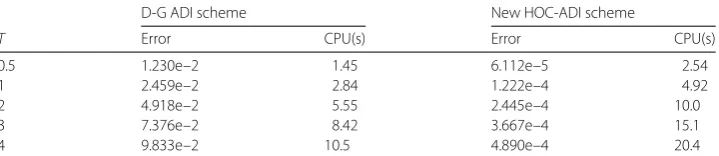
Table 2 Comparison of maximum errors at different timeTfor the equation in Example1,
h= 2π/20, time stepτ= 0.01
D-G ADI scheme New HOC-ADI scheme
T Error CPU(s) Error CPU(s)
0.5 1.230e–2 1.45 6.112e–5 2.54
1 2.459e–2 2.84 1.222e–4 4.92
2 4.918e–2 5.55 2.445e–4 10.0
3 7.376e–2 8.42 3.667e–4 15.1
4 9.833e–2 10.5 4.890e–4 20.4
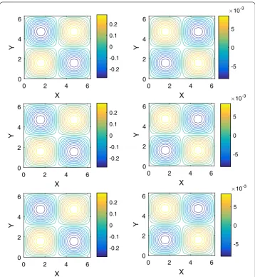
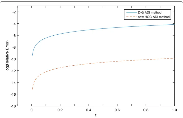
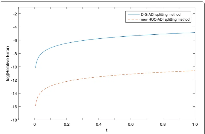
the maximum of numerical errors until timeT= 4 using two methods. Figure1shows the contour plot of exact solution and numerical solutions by the D-G ADI scheme and the new HOC-ADI scheme in thex–yplane atT = 0.01,z= 0.5 withN= 100 andM= 20. Figure2gives relative errors for the two methods, whereτ= 0.005,h= 2π/25. The relative errors are defined by
Relative Error =uexact(x,y,z,t) –uapprox(x,y,z,t)∞
uexact(x,y,z,t)∞ .
In Fig.3, we use the two methods to investigate the discrete mass and energy conservation errors for Example1, whereτ= 0.005,h= 2π/25. The errors are measured by
Error ofQ(t) =Qn–Qo, Error ofE(t) =En–Eo.
The results in Table1, Table2, and Fig.1show that the new HOC-ADI scheme is more accurate than the D-G ADI scheme, and the new HOC-ADI scheme and D-G ADI scheme have the orderO(τ2+h4) andO(τ2+h2), respectively. From Fig.3we can observe that two
schemes for this linear problem preserve the mass and energy conservation.
Example 2 (3D NLS equation) For this example, we consider the following three-dimensional NLS equation:
i∂u(x,y,z,t)
∂t = –
1 2
∂2
∂x2 +
∂2
∂y2+
∂2
∂z2
u(x,y,z,t)
+β u(x,y,z,t) 2u(x,y,z,t) +v(x,y,z)u(x,y,z,t), (x,y,z)∈[0, 2π]×[0, 2π]×[0, 2π],t∈(0,T],
Figure 1The contour plot of exact solution and numerical solutions to Example1atT= 0.01,z= 0.5 with N= 100 andM= 20. Left panel for real part and right panel for imaginary part correspond to the exact solution, solutions by the D-G ADI scheme, and solutions by the new HOC-ADI scheme, respectively)
wherev(x,y,z) = 1 –sin2xsin2ysin2zandβ= 1. The exact solution for this equation is in the following form:
uexact(x,y,z,t) =sinxsinysinzexp(–i5t/2).
We solved the equation by both D-G ADI splitting scheme (3.6) and the new HOC-ADI splitting scheme (3.7) with homogeneous boundary conditions. Table3illustrates the maximum error of|uexact(x,y,z,t) –uapprox(x,y,z,t)|and orders from the two methods at T= 2, and we can see that the new HOC-ADI splitting scheme and the D-G ADI splitting scheme have the orderO(τ2+h4) andO(τ2+h2), respectively. Table4shows the maximum
Figure 2Comparison of relative error using D-G ADI scheme and new HOC-ADI scheme for Example1
Figure 3Discrete conservation errors using two methods for Example1underτ= 0.005,h= 2π/25
Table 3 Numerical comparison results of the D-G ADI splitting scheme and the new HOC-ADI splitting scheme for Example2, atT= 2, time stepτ= 0.001
D-G ADI scheme New HOC-ADI scheme
h Error Order CPU(s) Error Order CPU(s)
π
5 6.790e–2 – 23.31 9.495e– – 36.56
π
10 1.709e–2 1.989 153.1 5.888e–5 4.011 218.7
π
20 4.281e–3 1.997 1123.0 3.672e–6 4.003 1547.4
π
40 1.071e–3 1.999 9307.0 2.294e–7 4.001 12,116.5
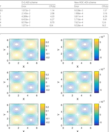
Table 4 Comparison of maximum errors at different timeTfor the equation in Example2,
h= 2π/15, time stepτ= 0.01
D-G ADI scheme New HOC-ADI scheme
T Error CPU(s) Error CPU(s)
0.5 1.072e–2 1.14 9.528e–5 1.57
1 2.145e–2 2.08 1.906e–4 3.16
2 4.289e–2 4.20 3.811e–4 6.29
3 6.433e–2 6.27 5.716e–4 9.41
4 8.576e–2 8.70 7.621e–4 12.6
5 1.071e–1 10.4 9.526e–4 16.5
Figure 4The contour plot of exact solution and numerical solutions to Example2atT= 0.01,z= 0.5 with N= 100 andM= 20. (Left panel for real part and right panel for imaginary part corresponding to the exact solution, solutions by the D-G ADI splitting scheme, and solutions by the new HOC-ADI splitting scheme, respectively)
5 Conclusions
Figure 5Comparison of relative error using D-G ADI splitting scheme and new HOC-ADI splitting scheme for Example2
Figure 6Discrete conservation errors using two methods for Example2underτ= 0.005,h= 2π/25
results show that the proposed methods are efficient and accurate for numerically solving 3D Schrödinger equations.
Acknowledgements
The authors would like to express their sincere thanks to the anonymous referees and associated editor for his/her careful reading of the manuscript.
Funding
This work is partially supported by the Natural Science Foundation of Xinjiang Province (No. 2017D01C052), the National Natural Science Foundation of China (No. 11671345), the Key Laboratory Project of Xinjiang Province (No. 2017D04030), Excellent Doctor Innovation Program of Xinjiang University (No. XJUBSCX-2013005).
Competing interests
Authors’ contributions
All authors have read and approved the final manuscript.
Publisher’s Note
Springer Nature remains neutral with regard to jurisdictional claims in published maps and institutional affiliations.
Received: 15 March 2018 Accepted: 26 June 2018
References
1. Arnold, A.: Numerically absorbing boundary conditions for quantum evolution equations. VLSI Des.6(1), 313–319 (2014)
2. Dodd, R.K., Eilbeck, J.C., Gibbon, J.D.: Solitons and Nonlinear Wave Equations. Academic Press, New York (1982) 3. Hajj, F.Y.: Solution of the Schrödinger equation in two and three dimensions. J. Phys.
4. Sulem, C., Sulem, P.L.: The Nonlinear Schrödinger Equation: Self-Focusing and Wave Collapse. Springer, New York (1999)
5. Akrivis, G.D.: Finite difference discretization of the cubic Schrödinger equation. IMA J. Numer. Anal.24(1), 115–124 (1993)
6. Bratsos, A.G.: A linearized finite-difference method for the solution of the nonlinear cubic Schrödinger equation. Korean J. Comput. Appl. Math.8(3), 459–467 (2001)
7. Dehghan, M.: Finite difference procedures for solving a problem arising in modeling and design of certain optoelectronic devices. Math. Comput. Simul.71(1), 16–30 (2006)
8. Dehghan, M., Shokri, A.: A numerical method for two-dimensional Schrödinger equation using collocation and radial basis functions. Comput. Math. Appl.54(1), 136–146 (2007)
9. Dehghan, M., Mirzaei, D.: Numerical solution to the unsteady two-dimensional Schrödinger equation using meshless local boundary integral equation method. Int. J. Numer. Methods Eng.76(4), 501–520 (2008)
10. Dehghan, M., Abbaszadeh, M., Mohebbi, A.: Numerical solution of system of n-coupled nonlinear Schrödinger equations via two variants of the meshless local Petrov–Galerkin (MLPG) method. Comput. Model. Eng. Sci.100(5), 399–444 (2014)
11. Bao, W., Cai, Y.: Uniform error estimates of finite difference methods for the nonlinear Schrödinger equation with wave operator. SIAM J. Numer. Anal.50(2), 492–521 (2012)
12. Chang, Q., Jia, E., Sun, W.: Difference schemes for solving the generalized nonlinear Schrödinger equation. J. Comput. Phys.148(2), 397–415 (1999)
13. Kurtinaitis, A.I.F.: Finite difference solution methods for a system of the nonlinear Schröinger equations. Nonlinear Anal., Model. Control9(3), 247–258 (2004)
14. Sulem, P.L., Sulem, C., Patera, A.: Numerical simulation of singular solutions to the twe-dimensional cubic Schrödinger equation. Commun. Pure Appl. Math.37(6), 755–778 (2010)
15. Dehghan, M., Mohebbi, A., Asgari, Z.: Fourth-order compact solution of the nonlinear Klein–Gordon equation. Numer. Algorithms52(4), 523–540 (2009)
16. Deng, D., Zhang, C.: Analysis and application of a compact multistep adi solver for a class of nonlinear viscous wave equations. Appl. Math. Model.39(3–4), 1033–1049 (2015)
17. Deng, D.: The study of a fourth-order multistep adi method applied to nonlinear delay reaction-diffusion equations. Appl. Numer. Math.96, 118–133 (2015)
18. Deng, D., Jiang, Y., Liang, D.: High-order finite difference methods for a second order dual-phase-lagging models of microscale heat transfer. Appl. Math. Comput.309, 31–48 (2017)
19. Wang, T., Guo, B., Xu, Q.: Fourth-order compact and energy conservative difference schemes for the nonlinear Schrödinger equation in two dimensions. J. Comput. Phys.243, 382–399 (2013)
20. Mohebbi, A., Dehghan, M.: The use of compact boundary value method for the solution of two-dimensional Schrödinger equation. J. Comput. Appl. Math.225(1), 124–134 (2009)
21. Mahdi, S.: Fourth order compact finite difference scheme for two dimension Schrödinger equation. Basrah J. Sci. 25(2), 142–149 (2007)
22. Xu, Y., Zhang, L.: Alternating direction implicit method for solving two-dimensional cubic nonlinear Schrödinger equation. Comput. Phys. Commun.183(5), 1082–1093 (2012)
23. Tian, Z.F., Yu, P.X.: High-order compact ADI (HOC-ADI) method for solving unsteady 2D Schrödinger equation. Comput. Phys. Commun.181(5), 861–868 (2010)
24. Gao, Z., Xie, S.: Fourth-order alternating direction implicit compact finite difference schemes for two-dimensional Schrödinger equations. Appl. Numer. Math.61(4), 593–614 (2011)
25. Liao, H., Sun, Z., Shi, H., Wang, T.: Convergence of compact ADI method for solving linear Schrödinger equations. Numer. Methods Partial Differ. Equ.28(5), 1598–1619 (2012)
26. Li, L.Z., Sun, H.W., Tam, S.C.: A spatial sixth-order alternating direction implicit method for two-dimensional cubic nonlinear Schrödinger equations. Comput. Phys. Commun.187, 38–48 (2015)
27. Kong, L., Duan, Y., Wang, L., Yin, X., Ma, Y.: Spectral-like resolution compact adi finite difference method for the multi-dimensional Schrödinger equations. Math. Comput. Model.55(5–6), 1798–1812 (2012)
28. Hendricks, C., Heuer, C., Ehrhardt, M., Günther, M.: High-order ADI finite difference schemes for parabolic equations in the combination technique with application in finance. J. Comput. Appl. Math.316, 175–194 (2017)
29. Strang, G.: On the construction and comparison of difference schemes. SIAM J. Numer. Anal.5(3), 506–517 (1968) 30. Wang, H.: Numerical studies on the split-step finite difference method for nonlinear Schrödinger equations. Appl.
Math. Comput.170(1), 17–35 (2005)