R E S E A R C H
Open Access
Cooperative spectrum-sensing algorithm
in cognitive radio by simultaneous sensing
and BER measurements
Yingqi Lu
1, Donglin Wang
1,2*and Michel Fattouche
1Abstract
This paper considers spectrum utilization, the probability of detection in cognitive radio (CR) model based on cooperative spectrum sensing with both simultaneous adaptive sensing and transmission at a transmitting secondary user (TSU), and the bit error rate (BER) detection with variation checking at a receiving user (RSU). In this paper, a novel detecting model is proposed in the being considered scenario for the full-duplex TSU’s simultaneous sensing and transmitting. A spectrum sensing scheme with an adaptive sensing window is designed to improve the spectrum utilization with a high SNR. At RSU, the BER variation is used further to detect whether a PU is active or not. Data fusion based on the proposed adaptive sensing scheme and the BER detection is processed for better decison on the spectrum holes. Simulation results show that (1) simultaneous spectrum sensing with an adaptive window improves the spectrum utilization compared with a periodical sensing and (2) cooperative spectrum sensing with the
BER-assisted detection improves the probability of detection and spectrum utilization compared with the single simultaneous sensing at TSU.
Keywords: Cognitive radio, Cooperative spectrum sensing, Spectrum utilization, Adaptive window, BER-assisted detection
1 Introduction
Cognitive radio (CR) is an important strategy to enhance spectrum efficiency, allowing the secondary user (SU) to utilize the licensed spectrum of the primary user (PU) when PU is inactive. This kind of time slot is called as a spectrum hole [1, 2]. CR has two important functionali-ties: spectrum sensing and adaption [1]. Energy detection is conventionally used for spectrum sensing [3]. Tradition-ally, SU firstly detects the spectrum band using energy collection periodically. If a spectrum hole is found, SU will immediately utilize this time interval to transmit data by upconverting to the PU’s frequency band. Once SU senses the activity of PU, it will immediately stop transmitting and give the spectrum back to PU. Then SU keeps detect-ing the spectrum in its own period till the comdetect-ing of next spectrum hole.
*Correspondence: [email protected]
1ECE Department, University of Calgary, 2500 University Drive, T2N 1N4 Calgary, Canada
2ECE Department, New York Institute of Technology, Old Westbury, NY, USA
Different from the model described above where SU executes sensing only when it does not transmit data [4, 5], a couple of full-duplex spectrum sensing schemes have been proposed in which the SU can simultaneously imple-ment transmitting and sensing whether PU is active or not. Researchers present a new design paradigm for future CR by exploring the full-duplex techniques to achieve the simultaneous spectrum sensing and data transmis-sion in [6] , published in a magazine to explore key research directions, and proposed an adaptive scheme to improve SUs’ throughput by switching between the “Listen-and-Talk” and “Listen-before-Talk” protocols in [7]. Non-time-slotted CR has been investigated in [8] and [9] and the full duplex spectrum sensing scheme is pre-sented for non-time-slotted cognitive radio networks in [8]. Afifi and Krunz [10] exploits self-interference sup-pression for improved spectrum awareness/efficiency in simultaneous transmit-and-receive mode. Results in [11] show the performance of antenna for the full-duplex
transmission in CR. The possibility of extending full-duplex designs to support multiple input, multiple out-put (MIMO) systems using commodity hardware has been discussed in [12]. Tsakalaki et al. [13] describes the basic design challenges and hardware requirements that restrain CRs from simultaneously and continuously sens-ing the spectrum while transmittsens-ing in the same frequency band.
This paper also considers the full-duplex spectrum sens-ing and utilization in CR. The besens-ing considered CR in this paper consists of two SUs. One SU transmits data and another SU receives the data. The SU which is used to transmit the data is called TSU while the one receiv-ing the data is called RSU. Both TSU and RSU are radio transceivers. In this paper, a novel detecting algorithm is proposed by combining an adaptive sensing in TSU and the BER detection in RSU, where a dedicated line is required for the transmission of the result of BER detec-tion to the TSU and data fusion is processed in the TSU. The difference of our algorithm from the existing full-duplex cognitive radio lies in the adaptiveness of the sensing window, the feedback of BER detection and the data fusion of the sensing in TSU and the BER detec-tion in RSU. One point to be noted is that we ignore the overhead effect in this paper because the data is less and negligible. The corresponding probability of detec-tion as well as the false alarm are provided, on the basis of which the utilization of spectrum holes is mathemat-ically derived. With the proposed spectrum detecting algorithm, a spectrum sensing scheme with an adaptive sensing window is designed to improve the spectrum utilization. Several schemes based on the adaptive sens-ing window have been proposed in literature [14, 15]. In this paper, the novel detection algorithm is followed by an adaptive spectrum sensing algorithm to provide an improved CR. Furthermore, in order to enhance the over-all detection accuracy, this paper feeds back the detection results based on the estimated bit error rate (BER) by RSU to TSU. By data fusion, this information is com-bined with the detection algorithm using an adaptive sensing window at TSU. The combined detection algo-rithm provides a better probability of detection and con-sequently a higher spectrum hole utilization. Although there is a trade-off between spectrum sensing and data transmission, it is also important to improve its spectrum utilization [16].
The rest of this chapter is organized as follows. Section 1 mentions the problems associated with recent develop-ments in spectrum sensing. Section 2 describes the system model and the spectrum sensing procedure that is pro-posed in our novel P2P cognitive radio. Section 3 shows the energy detection algorithm at TSU and derives its cor-responding probability of detection as well as false alarm, spectrum utilization and our proposed adaptive sensing
algorithm. Section 4 describes the detection algorithm that is based on estimating the BER at RSU. Section 5 gives the derivations of spectrum utilization under peri-odical sensing, simultaneously sensing with fixed win-dow and adaptive winwin-dow, as well as cooperative sensing with simultaneous sensing and BER detection. Simulation results are reported in Section 6 followed by a conclusion in Section 7.
2 Problem statement
Most existing spectrum-sensing technologies have two main problems. First, at TSU, periodical spectrum sens-ing cannot determine the periodical duration of spec-trum sensing. Here, we consider simultaneous specspec-trum sensing and transmitting. Secondly, spectrum sensing at TSU often brings miss-detection of PU signals when PU becomes a hidden node compared to TSU. Thus, we propose a novel BER-assisted detection to improve the spectrum sensing.
2.1 Simultaneous sensing/transmitting at full-duplex TSU
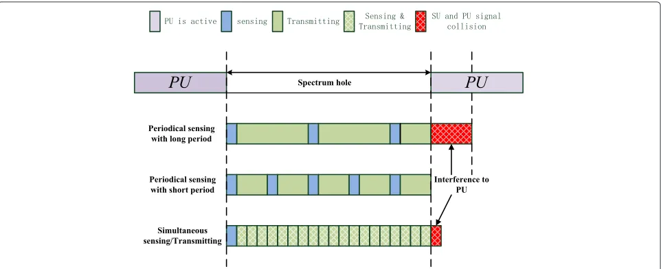
In the majority of existing spectrum-sensing technologies, spectrum sensing at TSU is executed periodically without the transmission of SU signals. However, this periodi-cal sensing exists a problem when selecting its periodiperiodi-cal duration. As shown in Fig. 1, if the duration is too long, the SU signal can represent interference to the PU sig-nal. It is obvious that this interference will decrease when the periodical duration decreases. However, if the period-ical duration is too short, it will cost more time to execute spectrum sensing instead of transmitting SU signals which will decrease the utilization of spectrum holes. In order to overcome this problem, we propose a solution to execute spectrum sensing while transmitting SU signals. When SU detects the existence of a spectrum hole, it transmits its signal over the licensed channel. Meanwhile, it will start to detect whether PU is active or not in order to min-imize interfering with the SU signal. TSU in cognitive radio is a full-duplex system which can transmit data while simultaneously perform spectrum sensing.
2.2 Assisting detection based on BER At SU receiver
We have proposed the concept of cooperative spectrum sensing between TSU and RSU based on estimating the BER at RSU. This is useful because a PU transmitter some-times becomes a hidden node compared to TSU which means that TSU cannot detect the existence of PU. There are two kinds of hidden nodes. The two cases are shown below.
2.2.1 Case I: TSU is out of the transmitting range of a PU transmitter
Fig. 1Periodical spectrum sensing and simultaneous sensing/transmitting. Compare the periodical spectrum and simultaneous sensing/transmitting at the same spectrum hole duration, we can find that the simultaneous sensing provides a higher spectrum utilization and less interference to PU
PU no matter whether PU is active or not. TSU will con-tinue to transmit data to its receiver. However, if RSU is in the transmitting range of a PU transmitter while hidden from it, the transmission between TSU and RSU can bring serious interference to PU.
2.2.2 Case II: PU signal is hidden from TSU
As shown in Fig. 3, the energy of the PU signal at TSU is lower than the minimum detection threshold possibly due to the existence of obstructions between TSU and PU. Thus, it is difficult to detect the existence of PU if the spectrum sensing only happens at TSU. In this case, there will still exist serious interference between RSU and
PU when RSU is close to PU and there is no obstruction between them.
From the two cases above, one can notice that it is necessary to assist spectrum sensing at TSU with addi-tional spectrum sensing at RSU based on BER measure-ment. If the BER at RSU is large enough, the presence of PU is detected even if the received energy of PU at TSU is below the detection threshold.
3 System model
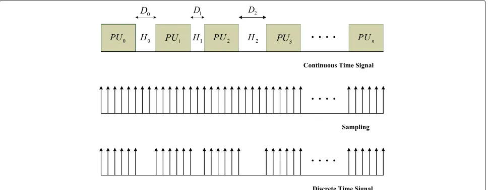
Spectrum sensing and transmitting at TSU in cognitive radio could be represented as shown in Fig. 4. Denoteh0,
h1, h2, · · ·, hm−1 as spectrum holes, i.e., PU is inactive
Fig. 3Hidden node case II. Both TSU and RSU are in the transmitting range of PU but there exists obstructions between TSU and PU
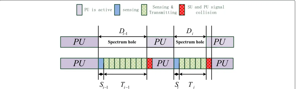
and the spectrum is idle during these time slots. The time duration of spectrum holehi is represented by Di, 0 ≤
i ≤ m−1, which is also the time interval between two adjacent transmissions by PU. In each spectrum hole, the TSU first senses whether the spectrum is being used or not. If the spectrum is unoccupied, the TSU borrows it to transmit data while simultaneously sense the start of a PU transmission. Therefore, the process consists of two stages: “sensing” only, followed by “transmitting and sens-ing”, as shown in Fig. 4.Sidenotes the duration that TSU takes to sense the spectrum before it can find a spectrum hole, and Ti represents the duration that TSU executes simultaneously sensing and transmitting. Spectrum sens-ing includes both spectrum senssens-ing at TSU by energy detection and spectrum sensing at RSU by BER estima-tion. The whole procedure of SU spectrum sensing and signal transmission can be summarized as follows:
• Step I: TSU senses the PU spectrum by energy detection.
• Step II: If TSU finds a spectrum hole, it awaits sensing of a spectrum hole at RSU by BER estimation. If not, it continues spectrum sensing by energy detection alone at TSU.
• Step III: If RSU also detects the existence of a spectrum hole, TSU starts to transmit data. At the same time, it continues to sense the spectrum band to detect when PU becomes active.
• Step IV: If TSU finds out that PU is active either by itself or with the help of RSU, it stops transmitting at once and goes back to Step I.
In the following section, we discuss spectrum sensing at TSU based on energy detection and at RSU based on BER estimation.
4 Energy detection at TSU
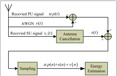
The block diagram corresponding to spectrum sensing using energy detection at TSU is shown in Fig. 5. The received signal is sampled to obtain a discrete time signal as shown in Fig. 6. Then, the system estimates the energy of the sampled signal during a sensing window. The length of the sensing window W can be a fixed value or a vari-able value. By comparing the threshold with the estimated energy, the system can conclude whether PU is active or not.
4.1 The energy detection algorithm and corresponding probability of detection at TSU
At theith “sensing” stage,Siin Fig. 4, the sensing signal at TSU can be expressed as:
y(n)=
v(n) forH0
αp(n)+v(n) forH1 , (1)
wherey(n), 0≤n≤N−1, denotes the received signal at TSU,N is the number of samples,αp(n)denotes the PU signal at TSU,v(n) denotes the AWGN with zero mean
Fig. 5The spectrum sensing system at TSU
and varianceσ2,α represents the channel gain between PU transmitter and TSU which depends on their relative positions and surrounding environment. HypothesisH0
indicates that PU is inactive while hypothesisH1indicates
that PU is active.
At theith “transmitting and sensing” stage,Tiin Fig. 4, the sensing signal at TSU can be expressed as:
y(n)=
s(n)+v(n) for H2
s(n)+αp(n)+v(n) for H3 , (2)
where y(n), p(n) ands(n), 0 ≤ n ≤ N − 1, have the same definition as the ones corresponding to the sens-ing stage, and s(n) denotes the received SU signal after going through the interference cancellation module in Fig. 7. HypothesisH2indicates that PU is inactive while
hypothesisH3indicates that PU is active. Without loss of
generality, it is assumed that p(n), s(n) and v(n) are all independent from each other.
The test statistic for energy detection under the four hypotheses,H0thoughH3, can be expressed as
T(y)= 1 W
W−1
n=0
|y(n)|2, (3)
wherey(n)is the TSU’s sensing signal as given in Eqs. (1) and (2), andW is the length of the sensing window, i.e., the number of baseband samples used for each detection decision. It can be described as:
W =fsτ, (4)
where fs is the sampling frequency at TSU and τ is the duration ofW. In order to estimate the energy, TSU esti-mates the energy for a time durationτ, which corresponds tofsτbaseband samples.
Fig. 7The duplex SU detector which applies antenna cancellation technique
Based on the theory described in [16], it is easily shown that the test statistic follows a normal distribution:
T(y)∼ denotes the power of the received PU’s signal,γ2 = σ
2
Based on Eqs. (5) and (6), at the “sensing” stage, the probability of detectionPd1 and of false alarmPf1 can be obtained as
where λ1 is the assumed threshold value which needs
to be selected appropriately and Q(·) represents the Q-Function.
Similarly, at the “sensing and transmitting” stage, the
probability of detectionPd2 and of false alarmPf2 can be obtained as
where λ2 is the assumed threshold value to be selected
appropriately. In the selection of thresholds, we hope to strike a balance between decreasing the probability of false-alarm and increasing the probability of detection. The threshold values λ1 and λ2 are constrained by the
equations below:
wherePm1 is the probability of miss-detection in hypoth-esisH1 whilePm2 is the probability of miss-detection in hypothesis H3. θ is a factor which is used to describe
the relationship between the miss-detection and the false alarm. It is called control factor. If θ is greater than 1, it means the probability of miss-detection is selected to be lower than the probability of false alarm. If θ is less than 1, it means the probability of miss-detection is selected to be greater than the probabil-ity of false alarm. If θ = 1, it means the probability of false alarm and the probability of miss-detection are selected to be the same. According to [14] and [17], we assume θ = 1 and substitute Eqs. (7)–(10) into (11). Then, we have
From Eq. (12), it is concluded that the threshold values λ1andλ2depend onσ2and on the SNRs:γ1,γ2andγ3,
but not on the length of the sensing windowW.
4.2 Discussion of power attenuation between PU and TSU
In this section, we discuss the power attenuation between PU and TSU according to the channel gain α between them. As previously discussed, we have known thatp(n)
denotes the amplitude of the PU signal at PU whileαp(n)
ρpu 1
W
W−1
n=0
|p(n)|2, (13)
ρsu 1
W
W−1
n=0
|αp(n)|2, (14)
whereρpurepresents the transmitting power at PU while
ρsu represents the received power at TSU. The relation-ship betweenρpuandρsuis as follows:
ρsu=α2ρpu, (15)
whereαdepends on the transmission channel which can include path-loss and shadow fading. According to a tra-ditional radio channel model, the equation to describe the fading of a radio signal can be expressed in a log scale (dB) as:
ρsu(dB)=ρpu(dB)−g1−g2log10zpu−zsu, (16)
wherezpuandzsurepresents the position of PU and TSU, respectively;zpu−zsuis the Euclidean distance which represents the relative distance,d,between PU and TSU whileρsu(dB)andρpu(dB) representsρsu andρpu in dB
g1/10 is called the fading constant, which is related to
shadow fading such as the position of obstructions in the transmission while g2/10 is a factor which depends on
the transmission environment and is referred to as path loss exponent. From Eq. (16), the channel gainα can be expressed as:
α2=10−g1/10d−g2/10, (17)
From Eqs. (15) and (17), one can expressα2as:
α2=PL−1zpu−zsu·ϕ=PL−1(d)·ϕ, (18)
where PL(d) = dg2/10 and ϕ = 10−g1/10. When the distance d becomes large, the value ofα2decreases. For Case I in Fig. 2, the path lossPL(d)is large when TSU is out of the transmission range of PU transmitter. Thus, the power gainα2 decreases to the point that TSU can-not detect the presence of PU. In Fig. 3, the value of ϕ is small because of obstructions between PU and TSU. Thus, the power gainα2is too small for PU signal to be detected.
4.3 Antenna cancellation technique in duplex TSU at P2P cognitive radio
In the P2P cognitive radio, because of the power atten-uation over the radio channel between PU and TSU, the power of the transmitted signals(n)at TSU, i.e., from its own transmit antenna, is much larger than the received signal at TSU from PUαp(n). This makes it difficult to realize a full duplex operation at TSU because of this large power difference. It is highly possible that TSU cannot
detect the energy of the weak received PU signal unless special care is undertaken. One way is to decrease such a power difference by makingαp(n)ands(n) of the same order of magnitude.
According to [18], a technique called antenna cancel-lation can be used for full-duplex operation. It com-bines the existing RF interference cancellation with digital baseband cancellation to reduce self-interference. Self-interference cancellation aims at decreasing the power difference between αp(n) and s(n). In Fig. 7, the value of s(n) is decreased to the same energy level as αp(n) using antenna cancellation technique. Thus, a full-duplex operation is enabled and TSU is able to detect the presence of PU while it is transmitting sig-nals. In other words, once the energy αp(n) is close to that of s(n), transmitting will not affect the detection of PU.
4.4 Spectrum sensing with adaptive window
In this section, we introduce the concept of an adaptive sensing window as applied to spectrum sensing based on energy detection, where the length of the sensing window,
W, varies fromWmaxtoWmin. Denote asWmaxthe maxi-mum allowed length of the sensing window. IfW>Wmax, there is no performance improvement. Denote as Wmin the minimum allowed length of the sensing window. If
W < Wmin, TSU cannot detect the PU signal due to an insufficient energy collection. In order to obtain a bet-ter sensing performance, the adaptive sensing algorithm is designed as follows:
• Step I: initialization - LetW =Wmaxso that TSU
can detect a real spectrum hole with high probability. • Step II: active PU - IfW >Wmin, assign
W =W−Wminto reduce the possibility of missing
spectrum holes with a small duration; ifW ≤Wmin,
assignW =Wmin.
• Step III: inactive PU - AssignW =Wmaxto enhance
the probability of detecting the coming PU.
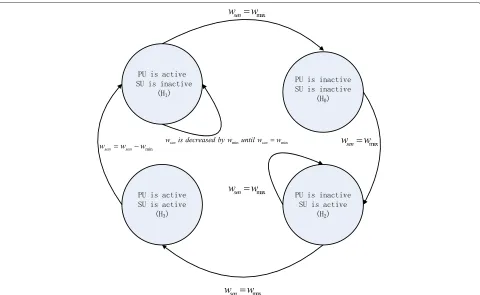
The state transition diagram in Fig. 8 can be used to represent the change in the value ofWwith the state tran-sition as a function of hypothesisH0toH3. The flowchart
of the adaptive sensing algorithm is shown in Algorithm 1. In this algorithm, we denotewcounteras a counter to keep track of the number of consecutive windows with an active PU and denoteCas the number of consecutive windows after which the length of the sensing window is decreased byWmin.
5 BER assisting detection at RSU
5.1 Novel TSU and RSU modules
Fig. 8State transition diagram among four hypothesis. The length of sensing windowWchanges betweenWmaxandWminwith the state transition
among hypothesisH0toH3
a new receiver architecture is proposed based on using a dedicated control channel.
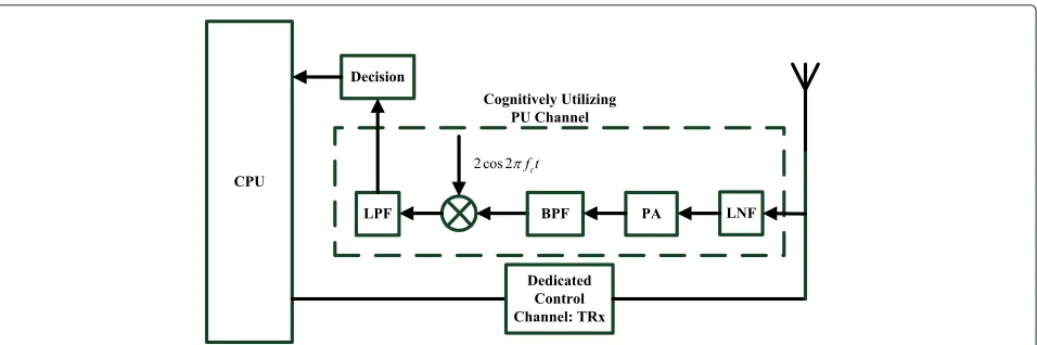
5.1.1 Proposed architecture for TSU
The proposed TSU architecture consists of three com-ponents as shown in Fig. 9. As previously discussed, one
component is used to sense PU’s activities, the second is used to transmit data by using the idle PU chan-nel while the last is used to exchange control informa-tion via a dedicated channel. The first component is used to estimate the energy of the received signal and to decide whether the PU channel is occupied or idle.
Algorithm 1 Spectrum sensing with adaptive window algorithm
1: W ←Wmax
2: wcounter←0
3: Initialize energy detection thresholdλ←λ1 4: ifT(y) < λthen
5: ifLast window find the spectrum holethen 6: Go to step 12;
7: else
8: W ←Wmax;
9: wcounter←0;
10: SU starts to transmit signal; 11: end if
12: λ←λ2; 13: Go to step 4;
14: else
15: ifLast window find PUthen 16: ifwcounter>=Cthen 17: ifW−Wmin<Wminthen
18: W ←Wmin;
19: else
20: W ←W−Wmin;
21: wcounter←0;
22: end if
23: else
24: wcounter←wcounter+1; 25: end if
26: else
27: SU stops transmitting;
28: W ←Wmax;
29: wcounter←0;
30: end if 31: Go to step 3 32: end if
This decision, as indicated by the dotted line in Fig. 9 controls a key “K1”; if the PU channel is idle, TSU starts to transmit data using the PU channel; otherwise, TSU does not transmit. The dedicated control chan-nel is used for transmitting the training sequence and for receiving the probability of detection based on BER estimation.
5.1.2 Proposed architecture for RSU
The corresponding RSU architecture consists of two components as shown in Fig. 10. The first compo-nent is used to receive the signal transmitted from TSU via the PU channel. The second component is the dedicated control channel which is used for receiv-ing the trainreceiv-ing sequence and for transmittreceiv-ing the esti-mated BER via a dedicated control channel. The BER is estimated using data sequences transmitted over the PU channel. These data sequences consist of useful information.
5.2 Modulation assumption
Without loss of generality, BPSK is assumed to be the modulation scheme for both TSU and PU. For analysis simplification, a perfect receiving process is considered and thus the continuous-time RF-received signal can be expressed as
y(t)=AP1(t)cos(2πfct)+v(t), (19)
whereAP1(t)=
−A Sending a bit “0”
A Sending a bit “1” for TSU signal,
whileAP1(t) =
−B Sending a bit “0”
B Sending a bit “1” for PU signal, where A and B are determined by their own transmit power and their propagation attenuation,fcis the carrier frequency andv(t)is the continuous-time white Gaussian noise with its discrete form v(n) in Eq. (1), with a zero
mean and a varianceσ2. It is also assumed that the
proba-bility of transmitting a bit “0” or “1” is equal for both TSU and PU, and that coherent detection is used at RSU.
5.3 BER with/without a PU signal
Without a PU signal, the BER is the well known BPSK expression given in [19], which is re-written here for convenience
where the optimal decision thresholdT =0 is used. On the other hand, when PU is active, the received signal at RSU can be expressed as
y(t)=AP2(t)cos(2πfct)+v(t), (21)
whereAP2(t)=
−A±B when TSU sends a “0”
A±B when TSU sends a “1”. The received signal after coherent detection is
ˆ ponent and quadrature component of v(t), a random process with a variance ofσ2. After the low-pass filter, the received signal can be obtained as
˜
The probability of error is derived below based on the probabilities in Eqs. (24) and (25). By choosing the deci-sion threshold value as T = 0, the probability of error decision when transmitting a bit “0”,Pˆe0, is given by
and the probability of error decision when transmitting a bit ‘1’,Pˆe1, is given by
Therefore, the overall BER can be obtained as
ˆ
5.4 Detection algorithm and probability of detection at RSU
Usually, a reliable communication system has a relatively low BER, e.g., lower than 10−3 level, [19], so Q Eq. (20) must be small. By looking at the Q-function table,
1 2
QA+σB+QA−σBin Eq. (26) is much higher than
QAσin Eq. (20). So, intuitively, the change of BER could be used for detecting the spectrum hole.
5.4.1 Method I
From Eqs. (20) and (26), one can conclude that BER estimation follows a nonnegative distribution with mean of QAσ for the case when PU is inactive and
1 2
QA+σB+QA−σBfor the case when PU is active. However, the variance is unknown and is represented by σb2 for both cases. Denote T as the threshold: if the BER measurement is greater than T, it says that PU is active; otherwise, it says that PU is inactive. The optimal threshold, T, must be selected in such a way that the minimum probability of decision error is reached. The probability of decision error PfT can be represented by
By calculating dPfT
Pf3 = P probability of detection Pd3 and a smaller probability of false alarm Pf3 .This makes sense because a higher
ˆ
Pe results in a bigger difference with Pe. It should be noted that whenPˆe >> Pe, the optimal threshold value
T ≈ Pˆe
2.
5.4.2 Method II
This algorithm is proposed by considering the ratio between the BER in Eq. (20) and the BER in Eq. (26), as a way to provide an obvious distinction between the two cases: inactive PU and active PU. The ratio of the real measurements of BER on Pe also follows a nonnegative distribution. The mean is obviously 1 for the case when
PU is inactive and Q for both cases. The optimal threshold corresponding to the minimum probability of decision error, which can be calculated as
Once again, by calculating dPˆfT
dT = 0, the optimal threshold value can be found, which can be approxi-mated as T = Pe+ˆPe
2Pe due to the low variance for this kind of measurements. As such, the probability of detec-tion and false alarm as defined in Secdetec-tion II can be represented by
which show the same performance as Method I.
5.5 Probability of detection based on a cooperative scheme between TSU and RSU
When TSU receives the BER which is estimated at RSU, it will make the final decision of whether PU is active or not based on a threshold. Here, we can obtain the prob-ability of detection based on such a cooperation between TSU and RSU. The condition for cooperative detection is that the spectrum hole is firstly detected at TSU. If PU is sensed by TSU, the training sequence will not be transmitted to RSU.
In hypothesisH1and hypothesisH3, the probability of
cooperative detection is the combination of two proba-bilities. The first is the probability of detection at TSU which we have already discussed in the previous section. The second is the probability when PU is detected at RSU though not at TSU. Thus, the probability of cooperative detection in hypothesis H1 andH3 can be expressed as
follows:
1 denotes the probability of cooperative detection in hypothesis H1 while Pcoopd2 represents the
probability of cooperative detection in hypothesis H2.
Because the probability of detection at TSU and the probability of detection at RSU are relatively inde-pendent, Eqs. (33) and (34) can be expressed as follows:
In Eqs. (35) and (36),Pd1 represents the probability of detection in hypothesisH1at TSU whilePd2 is the prob-ability of detection in hypothesisH3at TSU.Pd3 denotes the probability of detection based on BER estimation at RSU. All of these parameters have been discussed in the previous sections.
By the same principle, we can obtain the probabilities of false alarmPcoopf
1 andP coop
which are the probabilities that PU is detected though it is
According to the derivation from Eqs. (33)–(38), we can show that the new spectrum sensing scheme improves the probability of detection. It decreases the interference from SU. However, it also brings an increase in the prob-ability of false alarm which might decrease the spectrum utilization.
6 Spectrum utilization
6.1 Case I: ideally no noise or negligible noise
In order to measure spectrum utilization, and compare it to the traditional periodical sensing, it is necessary firstly to figure out how much time the “sensing” stage occupies and how much time the “transmitting” stage occupies dur-ing transmission. In our new full duplex TSU, it is also necessary to estimate the durations of the “sensing” stage “transmitting and sensing”. Assuming thatDH is the total duration of the spectrum holes in an observation interval, such as in Fig. 4, it can be written asDH = Ni=H0−1Di, where NH denotes the number of holes in the observa-tion interval, andDi, indicates the time duration of the
ithspectrum holehi. DenotingTHd as the total duration of the data transmission (i.e., the“transmitting ” stage in peri-odical sensing and the “transmitting and sensing” stage both at TSU) of all detected spectrum holes in an
obser-vation interval, it can be written as THd = N
d H−1 i=0 Ti, where NHd denotes the total number of spectrum holes detected by SU during the observation interval, whileTi, indicates the duration of the real data transmitting stage for theithspectrum holeh
i. Denoteηas the utilization of the spectrum holes. Spectrum utilization,η, can thus be calculated as
6.1.1 Ideally no noise or negligible noise in periodical spectrum sensing
In the traditional periodical spectrum sensing, the dura-tion of a spectrum hole, Di, which can be regarded as
a random variable, as in [16], follows an exponential distribution with an assumed mean μ. Its cumulative distribution function (CDF) can therefore be given as
FDi(D)=1−exp
−Dμ
, (40)
and its probability density function (PDF) can be described as
In addition,Tican also be regarded as a random vari-able, since:
Ti=Di−NiW =Di−DifsensW =Di(1−fsensW), (42)
wherefsensis the frequency of periodical spectrum sens-ing. It is a fixed value for a CR spectrum sensing system.
Niis the sensing instants in theith spectrum hole. In order to compute the CDF ofTi, for an arbitraryT,
Therefore, its CDF and PDF can be obtained, respec-tively, as
Furthermore, we have the expectation ofTi:
¯
One must note that fsensW ≤ 1 because the sensing periodf1
sensis always greater or equal to the lengthWof the sensing window. It is therefore reasonable to assume that when the sensing frequencyfsensincreases, the duration of data transmission decreases.
If there is no noise or negligible noise, each valid spec-trum hole is assumed to be detected. So, Eq. (39) can be written as
where W is a fixed value when the licensed channel is sensed by a sensing window with a fixed sized. In Eq. (47), one can conclude that the utilization of the spectrum decreases when the size of the sensing win-dow becomes larger. This result makes sense because the wasted time when the spectrum is not used is equal to the size of the sensing window during the sensing stage.
6.1.2 Ideally no noise or negligible noise when sensing and transmitting at the same time
Similar to traditional periodical spectrum sensing, the duration Di of a spectrum hole, at a full duplex TSU, can be regarded as a random variable foll an exponential distribution with an assumed mean μ whose cumula-tive distribution function (CDF) and probability density function (PDF) are shown in Eqs. (40) and (41).
Similarly, Ti can also be regarded as a random vari-able, indicating the duration of the “sensing and trans-mitting ” stage. In each spectrum hole, data transmission always happens except during the first spectrum sens-ing window. Thus, the transmission duration can be described as:
Ti=Di−W. (48)
In order to compute the CDF ofTi, for an arbitraryT, we have
P(Ti≤T)=P(Di≤T+W)=FD(T+W). (49)
Therefore, its CDF and PDF can be obtained, respec-tively, as
Furthermore, we have the expectation ofTias
¯
If there is no noise or negligible noise, each valid spec-trum hole is assumed to be detected. So, Eq. (39) can be written as sents the size of the first sensing window in one spectrum hole. The utilization of the spectrum also decreases when the size of the sensing windowW becomes larger. The size of the first sensing window is adaptive and change-able. Its range,Wadaptive should beWmin < Wadaptive <
Wmax. The aim of having an adaptive window is to decreaseWand improve spectrum utilization. It regulates the trade-off between the probability of detection and spectrum utilization because the probability of detection increases with W, while spectrum utilization decreases withW.
6.2 Case II: noisy environment
In general, there is non-negligible noise which increases the probability of false alarms. False alarms cause spec-trum holes not to be used. Thus, specspec-trum utilization is affected by the probability of false alarm.
First, when spectrum sensing is carried out only at TSU, spectrum utilization in Eq. (39) can be expressed as
ηnoise=
whereTilossdenotes the wasted durations in theith spec-trum holehiwhich are caused by false alarms whileD¯H =
μ,T¯Hd = ¯T− ¯Tloss,T¯lossis defined as the expected value of the wasted spectrum durationE{Tiloss}inith spectrum hole.
6.2.1 Noisy environment in periodical spectrum sensing In a periodical spectrum sensing scheme, E!Tiloss"
comes entirely from false-alarms during the “sens-ing” stage. It can be expressed as the expected value
E!Tilosssensing stage" of all wasted durations in one
period of spectrum sensing which denotes asW¯loss:
E!Tiloss"= ¯NE!Tilosssensing stage"= ¯NW¯loss, (54)
where N¯ is the expected value of the number of spec-trum sensing times in each specspec-trum hole. According to Eq. (42), we can obtain the expression below:
¯
Thus, the expected value of the number of spectrum sensing times in each spectrum holeN¯ is:
¯
N= 1 μ
fsens+ ¯Wloss
, (56)
probability of false alarmPf1. at TSU. It can be derived as
Here,Wis the size of the spectrum sensing window. Its value isW =Wmax. This is because, in our adaptive win-dow algorithm the size of the sensing winwin-dow does not change when PU is inactive.
According to Eqs. (55) and (56),E{Tiloss}is expressed as:
¯
Then, according to Eqs. (57) and (58), we can derive the utilization of the spectrumηperiodnoise in a periodical spectrum sensing system in a noisy environment as:
ηperiod
From Eq. (59), one can conclude that spectrum uti-lization ηperiodnoise decreases when the probability of false-alarm Pf1 increases. On the other hand, the utilization ηperiod
noise becomes lower when the size of the sensing win-dow W becomes larger which implies that Eq. (59) makes sense.
6.2.2 Noisy environment when sensing and transmitting at the same time
When sensing and transmitting at the same time in a full duplex TSU, the expected value of the wasted durations T¯duplexloss in each spectrum hole consists of two components. The first is the expected value of the wasted spectrum durations during the sensing stage. The other one is the wasted spectrum durations dur-ing the transmittdur-ing and sensdur-ing stage. In other words, we have
Tilosssensing and transmitting stage",
(60)
where Nduplex represents the number of sensing times in transmitting and sensing stage. In Eq. (60) ,
E{Tiloss|sensing stage}is the expected value of the wasted spectrum durations during the spectrum sensing in the sensing stage. Its expression is shown in Eq. (57). The sensing stage occurs once at the beginning of the spectrum hole.
In Eq. (60), E !
Tilosssensing and transmitting stage
"
denotes the expected value of the wasted spectrum dura-tions during the transmitting and sensing stage.
Similar to Eq. (57), we can obtain the expected value of the wasted spectrum durations during the transmitting and sensing stage as:
E!Tloss
i sensing stage and transmitting stage "
By comparing Eq. (57) with Eq. (61), one can see that the only difference betweenE!Tilosssensing stage"and
E{Tloss
i |transmitting and sensing stage}is that the proba-bility of false alarm in hypothesisH0is different from the
corresponding false alarm inH2.
In addition, in order to derive the utilization of a spec-trum hole, we need to know nduplex since the average duration of the “transmitting and sensing” stageT¯ is
¯
Thus,N¯duplexcan be expressed as:
¯
as the used spectrum in hypothesisH2. From Eq. (63), we
can obtain the following:
¯
We substitute Eqs. (51) and (64) into Eq. (53), to obtain an expression for the spectrum utilizationηduplexnoise :
ηduplex
In Eq. (65), when the probabilities of false alarmPf1and
Pf2 increase, the utilizationηduplexnoise becomes smaller. On the other hand, the utilizationηalso becomes lower when the size of the sensing windowW becomes larger. Thus, we can conclude that Eq. (65) makes senses.
6.3 Spectrum utilization in cooperative spectrum sensing between TSU and RSU
Next, we introduce the utilization of a spectrum hole when we use our new spectrum sensing scheme, i.e., when we combine BER estimation with energy detection to real-ize spectrum sensing. When we use the new spectrum sensing method, all relevant expressions are the same as Eqs. (60)–(65) except that we use Pfcoop
1 and P coop f2 to replace the originalPf1 andPf2. Moreover, the duration of the “transmitting and sensing” stage not only includes the wasted duration as well as the used spectrum in hypothesisH2, but also includes the length of the training
sequence which is used in BER estimation. So Eq. (62) can be rewritten as:
Here,W¯tsis the expected value of the length of the train-ing sequence andWts is the length of training sequence in each estimation of BER. Thus, the number of sensing timesN¯coopcan be expressed as:
¯
ThenT¯loss can be expressed according to Eqs. (66) and (67) as
Finally, it is easy to derive the utilization of the spectrum ηcoop
From Eqs. (68) and (69), we can conclude that the utilization of the spectrum depends on the probability of cooperative false-alarm Pfcoop
2 . The loss of spectrum
¯
Tlossbecomes larger when the cooperative probability of false-alarm at the “transmitting and sensing” stagePcoopf
for a CR full duplex system. IfPcoopf
2 increases, it implies that the CR transmitter will spend more time on spec-trum sensing instead of sensing and transmitting. In other words, some of the spectrum hole is missed without trans-mitting data at TSU. Thus, it is reasonable to assume that the utilization of the spectrumηcoopnoise decreases with the increase inPcoopf
2 in Eq. (69).
In addition, according to Eqs. (68) and (69), we can also conclude that spectrum utilizationηcoopnoiseis larger when the training sequenceWtsthat is used in BER estimation has a larger duration. However, it is possible that the longer length of the training sequence causes interference to PU especially at the end of a spectrum hole when PU might become active.
7 Numerical analysis and simulation results
7.1 Parameters
7.1.1 Basic parameters for the simulation
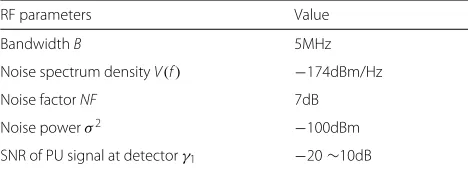
In this section, the proposed spectrum sensing at TSU is simulated using Matlab 2014b in a 64 bit computer with a core i7 and 8 GB RAM in order to demonstrate our proposed theory. The duration of a spectrum hole, which is also called appearance duration, follows an expo-nential distribution with a mean ofμ = 30000 samples. The arrival rate of a spectrum hole follows a Poisson distribution with an average arrival rate = 20000 sam-ples intervals. From [14], the maximum allowed length of the sensing windowWmax is 1000 samples. The min-imum allowed length of sensing window Wmin is 100 samples. The number of consecutive windows after which the length,C, of the sensing window is decreased byWmin, is set as 1, 2, or 5. In BER detection, the size of training sequence Wts is also 1000 samples. The RF parameters which include the bandwidth of the channelB, the ther-mal noise spectrum densityV(f), the noise factor of the receiverNFand the variance of AWGNσ2are all shown in Table 1.
7.1.2 Parameters for performance evaluation
The probability of detectionPd of a spectrum hole is an important factor when evaluating the performance of the proposed spectrum sensing algorithm. It is used to weigh the ability for TSU to avoid interfering with PU when PU is active. It is necessary to measurePdat TSU and RSU. That
Table 1RF simulation parameters
RF parameters Value
BandwidthB 5MHz
Noise spectrum densityV(f) −174dBm/Hz
Noise factorNF 7dB
Noise powerσ2 −100dBm
SNR of PU signal at detectorγ1 −20∼10dB
is why we need to obtain the probability of cooperative detection as well.
On the other hand, the probability of false alarm detec-tionPf is another important factor when PU is inactive. It affects the utilization of the spectrumη, which is another parameter when evaluating the performance of the pro-posed system. The utilization of the spectrum is also another parameter that plays a fundamental role in a CR system.
7.2 Probability of detection
In the simulations, we examine the probability of detec-tion at TSU first. As previously discussed, there exist two kinds of probabilities of detection and probabilities of false alarm: Pd1, Pf1 at “sensing" stage and Pd2, Pf2 at “sens-ing and transmitt“sens-ing” stage. Because the selection of the detection thresholdsλ1andλ2 is based on Eq. (12), the
value of Pd1 and of Pd2 increase while the value of Pf1 andPf2 decrease. Thus, when we evaluate the detection performance at TSU, we must examine the probability of detectionPd1andPd2 instead ofPd1,Pd2,Pf1, andPf2.
According to Eq. (7), Pd1 depends on the SNRγ1, the variance of the AWGN σ2 and the length of the sens-ing windowW.σ2is a constant in Table 1. The SNRγ1
depends on the PU transmitting power σp2 and factors which affect the channel gainαsuch as the transmission distanced, and shadow fadingϕin Eqs. (17) and (18). In our simulations, we evaluate the performance of CR for an SNR range from−20 to 10 dB. The length of the sensing windowW is regarded as a constant when the spectrum sensing work has a fixed window. The length of a fixed window is between Wmin andWmax. If spectrum sens-ing with an adaptive window as in Algorithm 1 is applied, the length of the sensing window will be a variable chang-ing from Wmax to Wmin. The simulation results on the probability of detection,Pd1, in Eq. (7) vs. SNR, γ1, are shown in Fig. 11. It makes sense that the probability of detection, Pd1, is always larger when W = Wmax than when W = Wmin. The reason is obvious: more energy is collected with a larger window, which has a higher probability to be greater than the preset threshold. When spectrum sensing uses an adaptive window, the average length of the sensing window for each sensing interval is betweenWmax andWmin. It depends on the value of C in Algorithm 1. The average W for each sensing inter-val becomes smaller asCbecomes larger. Thus, whenC
increases, it is reasonable to assume that the probability of detection Pd1 decreases. There is a gap between the
Fig. 11The probability of detectionPd1vs. SNRγ1. The probability of detection under hypothesisH1,Pd1, changes with different SNRγ1
theoretical result. Overall speaking, the simulation result approximately matches the derived theory (similar issue occurs again for the following simulation results).
Because a larger window leads to a better detection, for hypotheses H2/H3, the largest window W = Wmax is used to attain the best detection. Under this condition, the probability of detection,Pd1, in Eq. (7) for hypothe-sesH0/H1is compared with the probability of detection,
Pd2, in Eq. (9) for hypothesesH2/H3. Four cases are con-sidered: γ2
γ1 = 0.5, 1, 2, 4 with various transmitting power. Whenγ2
γ1 is greater than 1, it implies that the power of the SU signal is larger than the power of the PU signal. Fig. 12 shows the probability of detection versus SNRγ1. As seen,
Pd1 is always larger than the correspondingPd2 especially
Fig. 12The probability of detectionPd1andPd2vs. SNRγ1andγ2. The comparison ofPd1andPd2vs. SNRγ1are shown when the ratio of
γ2toγ1are 0.5, 1, 2, 4
when the TSU signal is larger than the PU signal. It is rea-sonable to assume that the PU signal is difficult to detect when the TSU signal is too large to exceed the PU signal. It also explains why we need to apply antenna cancella-tion techniques as previously discussed. It is reasonable to regardPd1as an approximation ofPd2when the PU signal αp(n)and the SU signals(n)are within the same or close order of magnitude. However, because both are based on energy detection,Pd1 and Pd2 are both imperfect when the SNR is relatively low. Thus, our proposed coopera-tive detection model provides a more precise detection. It requires detection at RSU which assists TSU in spectrum sensing.
From Section 4.4, the detection results at TSU depend on BER estimation using training sequences at RSU as well as using the optimal threshold which is a func-tion of the difference between the theoretical BER Pe when PU is inactive and Pˆe when PU is active. When the difference between Pe and Pˆe is large, it is easier to judge whether PU is active or not. From Eqs. (20) and (26), Pe and Pˆe are related to Aσ and σB. Because the variance of the AWGN σ2 is a fixed value,Pe and
ˆ
Pe depend on the relationship between the two signal amplitudes A and B. Here, we denote n = BA as the ratio between the PU signal amplitudeBand the SU sig-nal amplitude A. The difference between Pe and Pˆe vs. SNR are shown in Fig. 13. The difference between Pe andPˆe increases with the increase in n. This is reason-able because in this case PU adds more interference to the training sequence which causes bit errors when its transmitting power is large. In addition, whennis fixed, the difference betweenPeandPˆealso increases with the increase in SNR because the interference from the PU sig-nal is much larger than the effect of the AWGN. From Fig. 13,Pe andPˆe are always very close ifn = 0.25. In order to obtain a better detection based on BER estima-tion, we selectn=0.5, 1, 2 by transmitting power control signals.
According to our simulations, the probability of detec-tionPd3 based on BER estimation vs. SNR with different values ofn=0.5, 1, 2 is shown in Fig. 14.
In Fig. 14, increasingnimplies that the power of the PU signal becomes larger relative to that of the TSU signal. In this case, PU is easier to be detected which causesPd3
to increase. Actually, the ration between the PU signal power and the SU signal power can influence the exper-iment substantially. From Fig. 14, the simulation results are better than theory. This is reasonable because the the-oretical results are based on statistical assumptions while each instant of BER detection is carried out in a dis-crete and independent fashion in the simulations. Whenn
Fig. 13The Bit error ratePeandPˆevs. SNRγ1whenn=0.25, 0.5, 1, 2. The comparison ofPeandPˆevs. SNRγ1when the ratio of amplitudeBtoAare
0.25, 0.5, 1, and 2
simulation, we assume that the power of the SU signal is the same as the power of the PU signal. By comparingPd3 in Fig. 14 withPd1 andPd2 in Fig. 12, one can see that the detectionPd3 at RSU is greater than the detection at TSU in theory whenA ≥ BIt is helpful when a missed detection occurs at TSU such as in case I and case II in section 1.2.
So far, we have discussed the values ofPd1,Pd2, andPd3 vs. SNR. The probability of cooperative detection under hypothesis H1, Pcoopd1 and the probability of cooperative
detection under hypothesis H3, Pcoopd2 are presented in
Fig. 14The probability of detectionPd3and vs. SNRγ1when
n=0.5, 1, 2
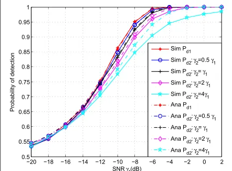
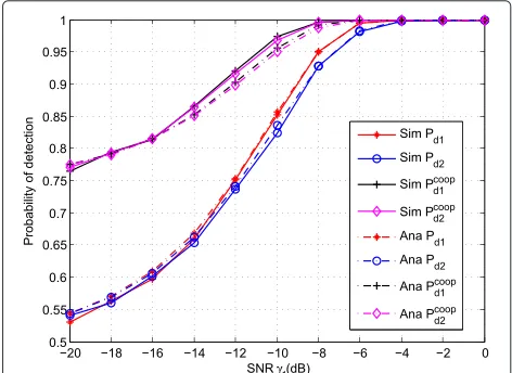
Fig. 15 using theoretical analysis from Eq. (35), Eq. (36), and practical simulation. They are to be compared with the probability of detectionPd1 andPd2. From Fig. 15, it is obvious that the performance of detection is improved using cooperative spectrum sensing between TSU and RSU, especially when the SNR is low. For instance, at an SNR = −20 dB, cooperative detection increases the probability of detection to around 77 from around 55 %. The probability of detection can be increased because a
Fig. 15The probability of detectionPd1,Pd2,P
coop d1 , andP
coop d2 vs. SNR
γ1. The probability of detectionPd1andPd2are compared with probability of cooperative detectionPdcoop
1 andP
missed detection at TSU is compensated by the detec-tion at RSU. When PU is not detected at TSU, there still exists a good probability for TSU to detect PU at RSU. Thus, the proposed cooperative detection at both ends of SU overcomes the shortcoming of energy detection and improves the performance of detection when the SNR is low. In addition, experimental results are better than the results obtained from theory because the theoreti-cal result are based on statistitheoreti-cal assumptions while each instant of spectrum sensing is carried out in a discrete and independent fashion in the simulations. The exper-imental results can not be fully described by theoretical analysis.
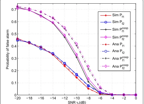
7.3 Probability of false alarm
False alarm happens when hypotheses H0 or H3 are
selected even though PU is inactive. It directly affects the utilization of the spectrum. When the probability of false alarm is high, a number of spectrum holes are missed by TSU. For this reason, we discuss the probability of false alarm before discussing the utilization of the spectrum. As in previous sections, the selection of the detection thresholdsλ1 andλ2 is based on Eq. (12). According to
Eqs. (37) and (38), the probabilities of false alarmPcoopf
1 and
Pfcoop
2 cannot be expressed byP coop d1 andP
coop
d2 directly even though they depend onPf1 andPf2. In Fig. 16, we com-parePfcoop
1 andP coop
f2 , withPf1 andPf2 which shows that the probability of false alarm increases when the coop-erative spectrum sensing is applied, especially when the SNR is low. Compared withPf1 andPf2, the total proba-bility of false alarmPcoopf
1 andP coop
f2 are greater because of the additional probability of false alarmPf3 at RSU. The simulation results are better than the theory because the
Fig. 16The probability of false alarmPf1,Pf2,P
coop f1 , andP
coop f2 vs. SNR
γ1. The probability of false alarmPf1andPf2are compared with probability of cooperative false alarmPcoopf
1 andP
coop f2
simulation results forPd1,Pd2andPd3are relatively higher than theory whilePf1,Pf2, andPf3 are relatively lower.
7.4 Spectrum utilization
In this section, we discuss the spectrum utilization by periodical spectrum sensing at TSU, simultaneously sens-ing/transmitting, and cooperative spectrum between TSU and RSU.
7.4.1 Simulation results for periodical sensing and simultaneous sensing
We first compare our proposed simultaneous sens-ing/transmitting with the traditional periodical sensing. For both cases, the sensing window is fixed. Its value is eitherWmax or Wmin. In periodical sensing, the ratio of the sensing window size W to the sensing period can be represented as fsensW. The value of fsensW is selected to be 23. Figure 17 indicates that the utilization of the spectrum ηnoiseduplex is always higher thanηperiodnoise in both simulation and theory. This is reasonable because the spectrum hole is not used to transmit data in each instance of periodical spectrum sensing while our pro-posed model can sense and transmit data at the same time. The duration of the wasted spectrum hole are shown as the blue blocks in Fig. 1. One can show that the simultaneous sensing/transmitting algorithm wastes less spectrum hole durations than periodical spectrum sensing.
When the SNR is relatively low (e.g., the SNR is from
−20 to−5 dB), in either of the two spectrum sensing algo-rithms, the utilization of spectrum becomes higher with the increase ofWfromWmintoWmax. This is reasonable because the probability of false alarm decreases and the probability of detection increases whenWincreases.
Fig. 17The utilization of spectrumηvs. SNRγ1when periodical and
When the SNR is greater than 0 dB, the spectrum uti-lization of periodical sensing ηnoiseperiodbecomes a constant value equal to 60 % regardless whether W is Wmax or
Wmin. In this case, the probability of false alarm is always 0 and the probability of detection is always 1 no matter how large the sensing window W is. ηperiodnoise depends on the ratio of sensing window size to sensing periodfsensW which is a constant.
For a fixed SNR greater than 0 dB, the spectrum utiliza-tion of simultaneous sensing/transmittingηnoiseduplexdepends on the duration of the only sensing stage. Figure 18 shows the spectrum holes before TSU senses and uses them in the simulation, and the usage of this spectrum after TSU senses and utilizes the spectrum holes. In each spectrum hole, the tiny white space shown in Fig. 18b is the only sensing stage which is at the beginning of each spectrum hole. The value of its duration depends on the correspond-ing size of the senscorrespond-ing window W. When W is larger, the spectrum utilization becomes lower. Thus, the energy detection withW = Wmaxhas the lowest utilization. Its bigger step causes more missing usage of the spectrum holes. Therefore, its spectrum utilization with high SNR cannot come close to 100 % (96.72 % from simulation). Conversely, energy detection withW =Wminleads to an approximate 100 % (99.67 % from simulation) hole utiliza-tion. It shortens the sensing durautiliza-tion. Hence, in order to obtain a high spectrum utilization at high SNR, we use the adaptive window algorithm to assist with simultaneous sensing at TSU.
7.4.2 Simulation on simultaneous sensing with adaptive window
Figure 19 indicates the comparison of spectrum utiliza-tion between sensing with a fixed window and sens-ing with an adaptive window. When C is reduced from 5 to 1, the sensing duration becomes smaller and the spectrum utilization becomes larger at high SNR. The best performance is obtained when C=1. In this case, the spectrum utilization improves from 96.72 % to 99.6 %.
Once again, the simulation results are better than the-ory because the expected value of the wasted dura-tion Tiloss in Eqs. (57) and (61) is larger than the one we obtain in the simulations. This is because it is less possible for false alarm to occur twice or more. The wasted duration in the simulations is mostly W
or 2W which is less than E!Tilosssensing stage" and
E!Tilosssensing stage and transmitting stage".
7.4.3 Simulation on cooperative spectrum sensing
Figure 19, indicates that the spectrum utilization is improved by using an adaptive window. In this case, spectrum utilization approaches 100 % when the SNR is between−5 and 10 dB. However, the spectrum utilization is still low when the SNR is between−20 and−10 dB. It is because we use energy detection to implement spectrum sensing at TSU. Energy detection has a poor detection per-formance when the SNR is low(i.e., it causes the increase of the probability of false alarm and the decrease of the
Fig. 19The utilization of the spectrumηvs. SNRγ1when simultaneous
spectrum sensing with fixed window and adaptive window are implemented
probability of detection). In order to improve the proba-bility of detection and consequently spectrum utilization, cooperative spectrum with BER estimation is introduced. In the simulations, Fig. 20 indicates that spectrum uti-lization at low SNR is improved when the BER is con-sidered as part of spectrum detection. For instance, at an SNR = −20dB, the proposed “adaptive sensing + BER” algorithm increases spectrum utilization from around 44 % to around 48 % using either a fixed or an adaptive sensing window in the simulations and increases spec-trum utilization from around 37 % to around 43 % in theory. Its spectrum utilization is greater than the peri-odical spectrum sensing.This is reasonable because, at low SNR, the BER detection uses the PU channel to transmit a training sequence. On one hand, the training sequence is used for PU detection in order to improve
Fig. 20The utilization of spectrumηvs. SNRγ1when sensing at TSU
with cooperative sensing between TSU and RSU
the probability of detection and decrease the probability of false alarm. On the other hand, the training sequence occupies the spectrum hole, which increases the spectrum utilization.
8 Conclusions
In this paper, a cooperative spectrum sensing between TSU and RSU is implemented in CR. Our novel adap-tive spectrum sensing scheme improves the spectrum utilization. Both the theoretical analysis and simulations show that the usage of an adaptive window improves the spectrum utilization from 96.72 to 99.6 %. Furthermore, BER-assisted detection greatly helps the adaptive spec-trum sensing. Simulation results demonstrate that coop-erative spectrum sensing can offer a better performance. It increases the utilization of the spectrum from around 44 % to around 48 % in the simulations and increases spectrum utilization from around 37 % to around 43 % in theory when SNR is−20dB.
Acknowledgements
A short version of this paper was presented in IEEE PIMRC 2014 [20].
Competing interests
The authors declare that they have no competing interests.
Received: 16 October 2015 Accepted: 9 May 2016
References
1. W Krenik, A Wyglinski, L Doyle, Guest editorial-cognitive radios for dynamic spectrum access. IEEE Commun. Mag.5(45), 64–65 (2007) 2. S Haykin, Cognitive radio: brain-empowered wireless communications.
Selected Areas Commun. IEEE J.23(2), 201–220 (2005)
3. JE Salt, HH Nguyen, Performance prediction for energy detection of unknown signals. Vehicular Technol. IEEE Trans.57(6), 3900–3904 (2008) 4. W Cheng, X Zhang, H Zhang, Full duplex wireless communications for
cognitive radio networks (2011). arXiv preprint arXiv:1105.0034 5. W Afifi, M Krunz, inDynamic Spectrum Access Networks (DYSPAN), 2014 IEEE
International Symposium On. Adaptive transmission-reception-sensing strategy for cognitive radios with full-duplex capabilities, IEEE, Tyson’s Corner, Virginia, USA, (2014), pp. 149–160
6. Y Liao, L Song, Z Han, Y Li, Full duplex cognitive radio: a new design paradigm for enhancing spectrum usage. Commun. Mag. IEEE.53(5), 138–145 (2015)
7. Y Liao, T Wang, L Song, Z Han, inGlobal Communications Conference (GLOBECOM), 2014 IEEE. Listen-and-talk: full-duplex cognitive radio networks, IEEE, Austin, USA, (2014), pp. 3068–3073
8. W Cheng, X Zhang, H Zhang, inMILITARY COMMUNICATIONS CONFERENCE, 2011-MILCOM 2011. Full duplex spectrum sensing in non-time-slotted cognitive radio networks, IEEE, Baltimore, USA, (2011), pp. 1029–1034 9. W Cheng, X Zhang, H Zhang, inProceedings of the 3rd ACM Workshop on
Cognitive Radio Networks. Imperfect full duplex spectrum sensing in cognitive radio networks (ACM, New York, USA, 2011), pp. 1–6 10. W Afifi, M Krunz, inINFOCOM, 2013 Proceedings IEEE. Exploiting
self-interference suppression for improved spectrum awareness/efficiency in cognitive radio systems, IEEE, Turin, Italy, (2013), pp. 1258–1266 11. E Ahmed, A Eltawil, A Sabharwal, inAntennas and Propagation Society
International Symposium (APSURSI), 2012 IEEE. Simultaneous transmit and sense for cognitive radios using full-duplex: A first study, IEEE, Memphis, USA, (2012), pp. 1–2
13. E Tsakalaki, ON Alrabadi, A Tatomirescu, E De Carvalho, GF Pedersen, Concurrent communication and sensing in cognitive radio devices: challenges and an enabling solution. Antennas Propag. IEEE Trans.62(3), 1125–1137 (2014)
14. D Treeumnuk, DC Popescu, inCommunications (ICC), 2012 IEEE International Conference On. Energy detector with adaptive sensing window for improved spectrum utilization in dynamic cognitive radio systems, IEEE, Ottawa, Canada, (2012), pp. 1528–1532
15. TS Shehata, M El-Tanany, inInformation Theory, 2009. CWIT 2009. 11th Canadian Workshop On. A novel adaptive structure of the energy detector applied to cognitive radio networks, IEEE, Ottawa, Canada, (2009), pp. 95–98
16. Y-C Liang, Y Zeng, EC Peh, AT Hoang, Sensing-throughput tradeoff for cognitive radio networks. Wireless Commun. IEEE Trans.7(4), 1326–1337 (2008)
17. DR Joshi, DC Popescu, O Dobre,et al, Gradient-based threshold adaptation for energy detector in cognitive radio systems. Commun. Lett. IEEE.15(1), 19–21 (2011)
18. JI Choi, M Jain, K Srinivasan, P Levis, S Katti, inProceedings of the Sixteenth Annual International Conference on Mobile Computing and Networking. Achieving single channel, full duplex wireless communication, ACM, New York, USA (ACM, New York, USA, 2010), pp. 1–12
19. TT Ha,Theory and Design of Digital Communication Systems. (ACM, New York, 2010)
20. Y Lu, D Wang, M Fattouche, inPersonal, Indoor, and Mobile Radio Communication (PIMRC), 2014 IEEE 25th Annual International Symposium On. Novel spectrum sensing scheme in cognitive radio by simultaneously sensing/transmitting at full-duplex tx and ber measurements at rx, IEEE, Pittsburg, USA, (2014), pp. 638–642
Submit your manuscript to a
journal and benefi t from:
7Convenient online submission 7Rigorous peer review
7Immediate publication on acceptance 7Open access: articles freely available online 7High visibility within the fi eld
7Retaining the copyright to your article