R E S E A R C H
Open Access
Robust stability analysis of impulsive
complex-valued neural networks with mixed
time delays and parameter uncertainties
Yuanshun Tan
1, Sanyi Tang
2*and Xiaofeng Chen
1*Correspondence:
2School of Mathematics and
Statistics, Shaanxi Normal University, Shaanxi, China
Full list of author information is available at the end of the article
Abstract
The robust stability for the impulsive complex-valued neural networks with mixed time delays is considered in this paper. Based on the homeomorphic mapping theorem, some sufficient conditions are proposed for the existence and uniqueness of the equilibrium point. By constructing appropriate Lyapunov–Krasovskii functions and employing modulus inequality techniques, the global robust stability theorem is obtained for the neural networks in complex domain. Finally, numerical simulations confirm the stability of the system and manifest that the complex-valued neural networks work efficiently on storing and retrieving the image patterns.
Keywords: Complex-valued neural networks; Modulus inequality techniques; Robust stability; Mixed time delays; Impulse
1 Introduction
Over the past few decades, the stability of real-valued neural networks (RVNNs) have been extensively investigated because of their widespread applications in various areas such as associative memory, pattern recognition, parallel computation, combinatorial op-timization and quantum communication [1–8], and a lot of existing work considers theμ -stability, power--stability, Lagrange stability and exponent-stability of the neural networks [9–13]. However, when designing neural networks, firstly the problem of robust stability should be investigated due to the parameter uncertainty in the system and the perturba-tion of parameters or system characteristics is often unavoidable. The reasons lie in two aspects: one is that the actual values of the characteristics or parameters will deviate from their initial values due to the inaccurate measurement, the other is that the characteristics or parameters will drift slowly in the course of system’s operation which is influenced by the environmental factors. These phenomena can be seen anywhere, such as image and signal processing, combinatorial optimization problems and pattern recognition [14]. So in recent years, the robustness of neural networks has become the most important topics in the control domain and attracted great attention of the scholars [12, 15–19].
For many applications of neural networks, the states are often objected to instantaneous disturbance and experienced abrupt changes at fixed time, which may be caused by switch-ing phenomenon, frequency changes or other sudden noise and often assumed to be in the form of impulses in the modeling process. Consequently, impulsive differential
tion provides a more natural description of such systems, the basic theorem of impulsive differential equation can be seen in [20]. There are also numerical and fruitful results as regards its applications; see [21–25] and the references therein. On the other hand, due to the neural processing and signal transmissions, the time delay is often occurred, and the existence of time delay may cause the instability and poor performance of the system [26]. For a specific neural network, delay may be caused by the measuring element or the mea-suring process, it may also be caused by the control element and the execution element. Strictly speaking, the time delay of the control system is common, therefore, many effort have been made devoted to the delay dependent stability analysis of neural networks [10, 27–30].
Comparing with RVNNs, the advantage of complex-valued neural networks (CVNNs) is that they can directly deal with the two-dimensional data, which can also be processed by RVNNs but needs double neurons. And in the application of CVNNS, the complex signals are proved to be more relevant [31–37], which is more natural to deal with the complex-valued date, weights and neuron activation functions. Consequently, as a class of complex-valued systems, CVNNs have received a growing number of studies and explored the application of neural networks. These fruitful results promote the rapid development of control theory. However, few articles consider the robust stability of neural networks with time delay and impulse in the complex domain. In [15], the authors investigated the existence, uniqueness and global robust stability of equilibrium point for complex-valued recurrent neural networks with time delays, in which the activation functions are sepa-rated by the real and imaginary parts, the analysis methods are skillful but cannot be used to dealt with complex-valued neural networks directly. In [19], the author also considered the dynamics of the same system, regretfully, the activation functions there are required to be bounded. So, the obtained stability criteria in [15, 19] cannot be applied if the acti-vation functions cannot be expressed by separating their real and imaginary parts or are unbounded. In [38], the robust stability with time delays and impulse in the complex do-main is considered, and the given stability criteria for complex-valued neural networks are obtained using different methods. However, the main conditions for the global ro-bust stability are restricted by two matrix inequalities, and there are only discrete delays in the model. Therefore, in this article, the robust stability of impulsive complex-valued neural networks with mixed time delays and parameter uncertainties is considered, the improved sufficient conditions are given for the existence, uniqueness and robust stabil-ity of the system in complex domain, moreover, numerical simulations manifest that the complex-valued neural networks work efficiently on storing and retrieving the image pat-terns.
The structure of this paper is arranged as follows. In Sect. 2, we introduce the CVNNs model and give some preliminaries, including some notations and important lemmas. The existence and uniqueness of the equilibrium will be proved using homeomorphic mapping principle in Sect. 3. The main part of Sect. 4 considers the global robust stability of the neu-ral networks by building the proper Lyapunov functions and using the modulus inequality technique. In Sect. 5, two numerical examples are presented to show the effectiveness of our theoretical analysis. Section 6 concludes the paper.
2 Problems formulation and preliminaries
real matrices and complex matrices. The subscripts T and ∗denote matrix transpo-sition and matrix conjugate transpotranspo-sition, respectively. For complex vectorz∈Cn, let |z|= (|z1|,|z2|, . . . ,|zn|)Tbe the module of the vectorz, andz=n
i=1|zi|2be the norm
of the vectorz. For complex matrixA= (aij)n×n∈Cn×n, let|A|= (|aij|)n×ndenote the
mod-ule of the matrixA, andA=ni=1nj=1|aij|2denote the norm of the matrixA.I
de-notes the identity matrix with appropriate dimensions. The notationX≥Y(respectively,
X>Y) means thatX–Yis positive semi-definite (respectively, positive definite). In addi-tion,λmax(P) andλmin(P) are defined as the largest and the smallest eigenvalue of positive
definite matrixP, respectively.
Motivated by [15], we will consider an impulsive complex-valued neural networks model with time delays whose dynamical behavior is governed by the following nonlinear differ-ential equations:
⎧ ⎪ ⎪ ⎨ ⎪ ⎪ ⎩ ˙
zi(t) = –dizi(t) +nj=1aijfj(zj(t)) +nj=1bijfj(zj(t–τj))
+nj=1cij t
–∞kj(t–s)fj(zj(s)) ds+Ji, t≥0,t=tk, zi(tk) =Iik(zi(t–
k)), k= 1, 2, . . . ,i= 1, 2, . . . ,n,
(1)
wherenis the number of the neurons,zi(t)∈Cdenotes the state of the neuroniat time
t,fj(t) is the complex-valued activation function,τj(j= 1, 2, . . . ,n) represents the discrete
transmission delay and satisfies 0≤τj≤ρ,di∈Rwithdi> 0 is the self-feedback
con-nection weight,aij∈Candbij∈Care the connection weights,kj(j= 1, 2, . . . ,n) is the distributed delay kernel function, Ji∈Cis the external input. Here Iik is a linear map,
zi(tk) =zi(tk+) –zi(tk–) is the jump ofziat momentstk and 0 <t1<t2<· · · is a strictly increasing sequence such thatlimk→∞tk= +∞.
Now we can rewrite (1) in an equivalent matrix-vector form as follows:
⎧ ⎨ ⎩ ˙
z(t) = –Dz(t) +Af(z(t)) +Bf(z(t–τ)) +C–∞t K(t–s)f(z(s)) ds+J,
z(tk) =I(z(t–
k)), k= 1, 2, . . . ,
(2)
where z(t) = (z1(t),z2(t), . . . ,zn(t))T ∈ Cn, D= diag{d1,d2, . . . ,dn}, A = (aij)n×n∈ Cn×n,
B = (bij)n×n ∈ Cn×n, f(z(t)) = (f1(z1(t)),f2(z2(t)), . . . ,fn(zn(t)))T, f(z(t – τ)) = (f1(z1(t – τ1)),f2(z2(t –τ2)), . . . ,fn(zn(t – τn)))T, K(t –s) = diag{k1(t –s),k2(t – s), . . . ,kn(t– s)}, J= (J1,J2, . . . ,Jn)T∈Cn,z(tk) = (z1(tk),z2(tk), . . . ,zn(tk))T, andI(z(t–k)) = (I1k(z(tk–)), I2k(z(tk–)), . . . ,Ink(z(tk–)))T.
We assume that system (1) or (2) is supplemented with the initial values given by
zi(s) =ϕi(s), s∈(–∞, 0],i= 1, 2, . . . , (3)
or in an equivalent vector form
z(s) =ϕ(s), s∈(–∞, 0], (4)
where ϕi(·) is complex-valued continuous function defined on (–∞, 0], and ϕ(s) =
(ϕ1(s),ϕ2(s), . . . ,ϕn(s))T∈C((–∞, 0],Cn) with the normϕ(s)=sups∈(–∞,0]ni=1|ϕi(t)|2.
Let us define a partial orderoverC: Forz1,z2∈C,z1z2if and only ifx1≤x2and
orderoverCn×n: ForA,B∈Hn×n,ABif only ifaijbij,i,j= 1, 2, . . . ,n, whereA= (aij)n×nandB= (bij)n×n.
The following assumptions will be needed throughout the paper:
(H1) The parametersD,A,B,C,Jin CVNNs (2) are assumed to be in the following sets, respectively:
DI= D∈Rn×nd : 0 <Dˇ D ˆD,
AI= A∈Cn×n:Aˇ A ˆA,
BI= B∈Cn×n:BˇB ˆB,
CI= C∈Cn×n:CˇC ˆC,
JI= J∈Cn:JˇJ ˆJ,
whereDˇ,Dˆ ∈Rn×nd ,Aˇ,Aˆ,Bˇ,Bˆ,Cˇ,Cˆ∈Cn×n, andJˇ,Jˆ∈Cn. Moreover, letAˇ= (aijˇ )n×n, ˆ
A= (aijˆ )n×n, Bˇ = (bijˇ )n×n, Bˆ = (bijˆ )n×n, Cˇ = (cijˇ )n×n, and Cˆ = (ˆcij)n×n. Then de-fine A˜ = (aij˜ )n×n, B˜ = (bij˜ )n×n and C˜ = (cij˜ )n×n, where aij˜ =max{|ˇaij|,|ˆaij|}, bij˜ = max{|ˇbij|,|ˆbij|},cij˜ =max{|ˇcij|,|ˆcij|}.
(H2) Forj= 1, 2, . . . ,n, the neuron activation functionfjis continuous and satisfies
fj(z1) –fj(z2)≤γj|z1–z2|,
for anyz1,z2∈C, whereγjis a real constant. Furthermore, define= diag{γ1,γ2,
. . . ,γn}.
(H3) Forj= 1, 2, . . . ,n, the delay kernelkjis a real value non-negative continuous function defined on[0, +∞)and satisfies,
+∞
0
kj(s) ds= 1,
+∞
0
sk(s) ds< +∞.
Remark1 For assumption (H1), the matrix intervalsDI,AI,BI,CI andJI represent the
allowed ranges of the parameters of the designed system due to parameter uncertainties caused by inaccurate measurements or environmental factors. For assumption (H2), the
assumption of Lipschitz condition is very general since the common activations, such as piece-wise linear function, logistic sigmoid function and hyperbolic tangent function, all satisfy the Lipschitz condition. For assumption (H3), it is a standardization assumption
for delay kernel functions. If the delay kernel functionkj˜ satisfies0∞kj˜(s) ds=K< +∞,kj
will satisfy assumption (H3) by lettingkj=kj˜/K.
Definition 1 A functionz(t)∈C((–∞, +∞),Cn) is a solution of system (2) satisfying the
initial value condition (4), if the following conditions are satisfied:
(i) z(t)is absolutely continuous on each interval(tk,tk+1)⊂(–∞, +∞),k= 1, 2, . . ., (ii) for anytk∈[0, +∞),k= 1, 2, . . .,z(tk+)andz(tk–)exist andz(t+k) =z(tk).
Definition 2 The neural network defined by (1) with the parameter ranges defined by (H1) is globally asymptotically robust stable if the unique equilibrium point zˇ =
Lemma 1([39]) For any a,b∈Cn,if P∈Cn×nis a positive definite Hermitian matrix,then a∗b+b∗a≤a∗Pa+b∗P–1b.
The following modulus inequalities of complex numbers play a central role for the re-sults of the paper.
Lemma 2 Suppose A∈Cn×n,Aˇ = (aˇij)n×n∈Cn×n,Aˆ = (aˆij)n×n∈Cn×n,andAˇ A ˆA. Then,for any x,y∈Cn,the following inequalities hold:
x∗A∗Ax≤ |x|∗|A|∗|A||x| ≤ |x|∗A˜∗A˜|x|, (5)
whereA˜= (aij˜ )n×n,aij˜ =max{|ˇaij|,|ˆaij|}.
Proof By Cauchy–Schwarz inequality, the modulus inequalities (5) can be obtained. The
proof is direct so we omit the details.
Lemma 3([39]) A given Hermitian matrix
S=
S11 S12 S21 S22
< 0,
where S∗11=S11,S∗12=S21and S∗22=S22,is equivalent to any one of the following conditions: (i) S22< 0andS11–S12S–1
22S21< 0, (ii) S11< 0andS22–S21S11–1S12< 0.
Lemma 4([39]) If H(z) :Cn→Cnis a continuous map and satisfies the following condi-tions:
(i) H(z)is injective onCn, (ii) limz→∞H(z)=∞,
then H(z)is a homeomorphism ofCnonto itself.
3 Existence and uniqueness of equilibrium point
In this section, we will derive sufficient conditions for the existence and uniqueness of equilibrium point of system (2). An equilibrium solution of (2) is a constant complex vec-torzˇ∈Cnwhich satisfies
–Dˇz+Af(zˇ) +Bf(ˇz) +Cf(zˇ) +J= 0, (6)
when the impulsive jumpsIk(·) as assumed to satisfyIk(ˇz) = 0,k= 1, 2, . . . .
Hence, to prove the existence and uniqueness of a solution of (6), it suffices to show that the following mapH:Cn→Cnhas a unique zero point,
H(z) = –Dz+Af(z) +Bf(z) +Cf(z) +J. (7)
Theorem 1 For the CVNNs defined by(2),assume that the network parameters and the activation function satisfy conditions(H1), (H2)and(H3). Then the neural network(2) has a unique equilibrium point for every input vector J= (J1,J2, . . . ,Jn)T∈Cn,if there exist two real positive diagonal matrices U and V such that the linear matrix inequality(LMI)
holds:
–DUˇ –UDˇ +V U(A˜+B˜+C˜) (A˜∗+B˜∗+C˜∗)U –V
< 0, (8)
whereA˜ = (a˜ij)n×n,B˜ = (b˜ij)n×n,C˜ = (˜cij)n×n,a˜ij=max{|ˇaij|,|ˆaij|},b˜ij=max{|ˇbij|,|ˆbij|}and ˜
cij=max{|ˇcij|,|ˆcij|}.
Proof To prove the existence and uniqueness of system (2), it suffices to showH(z) is a homeomorphism of Cnonto itself by using the homeomorphic mapping theorem on
complex domain.
First, we prove thatH(z) is an injective map onCn. Suppose that there existz,z˜∈Cn
withz=z˜, such thatH(z) =H(z˜). Then we can write
H(z) –H(z˜) = –D(z–z˜) + (A+B+C)f(z) –f(˜z)= 0. (9)
Multiplying both sides of (9) by (z–z˜)∗U, we can obtain
0 = –(z–z˜)∗UD(z–z˜) + (z–˜z)∗U(A+B+C)f(z) –f(z˜). (10)
Then, taking the conjugate transpose of (10) leads to
0 = –(z–z˜)∗DU∗(z–˜z) +f(z) –f(z˜)∗A∗+B∗+C∗U∗(z–˜z). (11)
Summing (10) and (11), applying Lemmas 1 and 2, we have
0 = –(z–z˜)∗(UD+DU)(z–z˜)
+ (z–z˜)∗U(A+B+C)f(z) –f(z˜)
+f(z) –f(z˜)∗A∗+B∗+C∗U(z–z˜)
≤–(z–z˜)∗(UD+DU)(z–z˜)
+ (z–z˜)∗U(A+B+C)V–1A∗+B∗+C∗U(z–z˜)
+f(z) –f(z˜)∗Vf(z) –f(z˜)
≤ |z–z|˜∗–DUˇ –UDˇ +U(A˜+B˜+C˜)V–1A˜∗+B˜∗+C˜∗U|z–z|˜
+f(z) –f(z˜)∗Vf(z) –f(z˜). (12)
SinceVis a positive diagonal matrix, from assumption (H2), we can get
f(z) –f(˜z)∗Vf(z) –f(z˜)≤(z–z˜)∗V(z–˜z)
It follows from (12) and (13) that
0≤ |z–z|˜∗ϒ|z–z|˜, (14)
whereϒ= –DUˇ –UDˇ+V+U(A˜+B˜+C˜)V–1(A˜∗+B˜∗+C˜∗)U. From Lemma 3 and the
LMI (8), we can see thatϒ< 0. Thenz–z˜= 0 from (14). Therefore,H(z) is an injective map onCn.
Second, we proveH(z) → ∞asz → ∞. LetH(z) =H(z) –H(0). By Lemma 1 and 2, we have
z∗UH(z) +H(z)∗Uz
= –z∗(UD+DU)z+z∗U(A+B+C)f(z) –f(0)
+f(z) –f(0)∗A∗+B∗+C∗Uz ≤–z∗(UD+DU)z
+z∗U(A+B+C)V–1A∗+B∗+C∗Uz
+f(z) –f(0)∗Vf(z) –f(0)
≤ |z|∗–DUˇ –UDˇ +U(A˜+B˜+C˜)V–1A˜∗+B˜∗+C˜∗U|z|+|z|∗V|z| ≤ |z|∗ϒ|z| ≤–λmin(–ϒ)z2.
An application of the Cauchy–Schwartz inequality yields
λmin(–ϒ)z2≤2z∗UH(z).
Whenz= 0, we have
H(z)≥λmin(–ϒ)z
2U .
Therefore,H(z) → ∞ asz → ∞, which implies H(z) → ∞asz → ∞. From Lemma 4, we know thatH(z) is a homeomorphism ofCn. Thus, the system (2) has a unique
equilibrium point. The proof is completed.
4 Global robust stability results
In the preceding section, we have shown the existence and uniqueness of the equilibrium point for system (2). In this section, to investigate the global robust stability of the unique equilibrium point, we should give the following assumption for the impulsive operators:
(H4) Fori= 1, 2, . . . ,nandk= 1, 2, . . ., the impulse operatorIik(·)satisfies
Iik
zi
tk–= –δik
zi
t–k–zˇi
,
Remark2 For (H4), the assumption can guarantee that the impulse is zero at the
equilib-rium point, i.e.,Iik(zˇ) = 0, which is one of the necessary conditions such that the equilib-rium point is asymptotically robust stable.
Theorem 2 Suppose the conditions(H1), (H2)and(H3)are satisfied.There exist four real positive diagonal matrices P,Q,R and S such that the following LMI holds:
= librium pointzˇ.Furthermore,if the condition(H4)is satisfied,the equilibrium pointz isˇ globally asymptotically robust stable.
Proof The theorem will be proved in two steps.
Step 1: We will show system (2) has a unique equilibrium point under LMI (15) by the matrix congruence method. Let
whereIis an identity matrix of ordern. It should be noted thatTis invertible and
1=T∗T.
Thus1andare congruent, which means that1is negative definite sinceis negative
definite. It should be also noted that2 is a principal submatrix of1. Therefore2is
negative definite, i.e.,
2< 0. (16)
Based on (16), we can see that there existU=P> 0 andV=S+Q+R> 0 such that LMI (8) holds. Consequently, system (2) has a unique equilibrium pointˇzby Theorem 1.
and then the system (2) can be transformed into
of (17), applying Lemmas 1 and 2, we get
+PCR–1C∗Pz˜(t)+g∗z˜(t–τ)Qgz˜(t–τ)
It follows from (23), (24) and (25) that
=
It follows from (26) and (27) thatV(t) is non-increasing fort≥0. According to assump-tion (H3), we can let
From (28) and (29), we obtain
z˜(t)≤
from which it can be concluded that the origin of (17), or equivalently the equilibrium point of system (2), is globally asymptotically robust stable by standard Lyapunov
theo-rem.
Corollary 1 Suppose the conditions(H1), (H2)and(H3)are satisfied.There exist four real positive diagonal matrices P,Q,R and S such that the LMI(15)holds.Then system(30)
has a unique equilibrium point which is globally asymptotically robust stable.
If the impulsive operatorI(·)≡0 andC≡0 in (2), we get the following complex-valued neural networks with discrete time delays:
˙
z(t) = –Dz(t) +Afz(t)+Bfz(t–τ)+J, (31)
whereD,A,B,Jandf(·) are defined as same as in (2). According to Theorem 2, we can obtain the following corollary on the global robust stability conditions of (31).
Corollary 2 Suppose the conditions(H1)and(H2)are satisfied.There exist three real pos-itive diagonal matrices P,Q and S such that the following LMI holds:
=
⎛ ⎜ ⎝
11 PA˜ PB˜
–S 0
–Q
⎞ ⎟
⎠< 0, (32)
where11= –DPˇ –PDˇ +(S+Q),A˜ = (aij˜ )n×n, B˜ = (bij˜ )n×n, aij˜ =max{|ˇaij|,|ˆaij|}and ˜
bij=max{|ˇbij|,|ˆbij|}.Then system(31)has a unique equilibrium point which is globally asymptotically robust stable.
IfDˇ=D=Dˆ,Aˇ=A=Aˆ,Bˇ=D=Bˆ,Cˇ =C=Cˆ andJˇ=J=Jˆin condition (H1), the
asymp-totical robust stability will reduced to the asympasymp-totical stability by Definition 2. Therefore, according to Corollaries 1 and 2, we can obtain the following corollaries on the global asymptotical stability conditions of (30) and (31).
Corollary 3 Suppose the conditions(H2)and(H3)are satisfied.There exist four real pos-itive diagonal matrices P,Q,R and S such that the following LMI holds:
=
⎛ ⎜ ⎜ ⎜ ⎝
11 P|A| P|B| P|C|
–S 0 0
–Q 0
–R
⎞ ⎟ ⎟ ⎟
⎠< 0, (33)
where11= –DP–PD+(S+Q+R).Then system(30)has a unique equilibrium point, which is globally asymptotically stable.
Corollary 4 Suppose the condition(H2)is satisfied.There exist three real positive diagonal matrices P,Q and S such that the following LMI holds:
=
⎛ ⎜ ⎝
11 P|A| P|B|
–S 0
–Q
⎞ ⎟
⎠< 0, (34)
Remark 3 In [40, 41], the criteria for stability of CVNNs are expressed in terms of complex-valued LMIs. As pointed out in [40], the complex-valued LMIs cannot be solved by MATLAB LMI Toolbox straightforwardly. An feasible approach is to convert complex-valued LMIs to real-complex-valued ones but this could double the dimension of the LMIs. In this paper, we express the stability criteria for CVNNs directly by terms of real-valued LMIs, which can be solved by MATLAB LMI Toolbox straightforwardly.
Remark 4 In [15], the authors investigate the problem of global robust stability of complex-valued recurrent neural networks with time delays and uncertainties. In The-orem 3.4 of [15], to check robust stability of complex-valued neural networks, the bound-edness of activation functionfiis required. However, in this paper, the boundedness con-dition is removed. See in Example 1 of next section the activation functionfiis unbounded.
5 Numerical examples
In this section, we will give two numerical examples to demonstrate the effectiveness and superiority of our results.
Example1 Assume that the network parameters of system (2) are given as follows:
ˇ the delay kernel functionsk1(·) andk2(·) satisfy assumption (H3), and the impulsive
func-tionsI1k(·) andI2k(·) satisfy assumption (H4) fork= 1, 2, . . . .
Thus, the specified network has a unique equilibrium point which is globally robust asymptotically stable. To perform numerical simulation, let us chooseD,A,BandCfrom the indicated intervals above, respectively, and obtain
D=
3 0 0 3
, A=
3 – 2i 1 + i –2 – i –1.5 + i
, B=
2 – 1.5i 1 + 1.5i 1.5 – 2i 2 + i
,
C=
1 + 1.2i 0.6 – 0.8i 1 – i 1.5 – 1.5i
, J=
3 – 2i 2 + 3i
.
(35)
Besides, we choose discrete delays, activation functions, delay kernel functions and im-pulse functions as follows:
τ1=τ2= 0.5, (36)
f1(u) =f2(u) = 0.2max{0,x}+max{0,y}, u=x+yi∈C, (37)
k1(s) =k2(s) =e–s, s∈[0, +∞), (38)
Iikzit–k= –δik
zitk––ziˇ, i= 1, 2, (39)
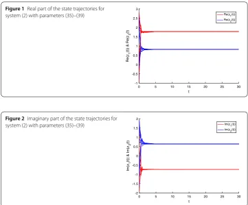
whereˇz1= 1.7813 – 0.7372i,ˇz2= 0.8132 + 0.6370i,δ1k= 1 +12sin(1 +k),δ2k= 1 +23cos(2k3), k= 1, 2, . . . , andt1= 0.5,tk=tk–1+ 0.2k,k= 2, 3, . . . . Figure 1 and 2 depict the real and imaginary parts of states of the considered system (2) with parameters (35)–(39), where the initial conditions are chosen by 10 random constant vectors.
Figure 1Real part of the state trajectories for system (2) with parameters (35)–(39)
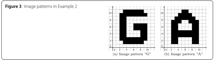
Figure 3Image patterns in Example 2
Remark5 In [15], the problem of global robust stability of CVNNs with discrete time delays but without distributed time delays. So the stability criteria obtained in [15] cannot be applied to check the robust stability of the system in Example 1.
Next we give a second numerical example on application of associative memories based on CVNNs.
Example2 Consider the image patterns “G” and “A” shown in Fig. 3 and design CVNNs in the form of (31) for associatively memorizing the images.
It should be noted that, as shown in Fig. 3, “G” and “A” are composed of 52 and 50 black block, respectively. Therefore, we need to design CVNNs (31) composed of 52 neurons, which have a 52-dimensional equilibrium point storing the coordinates of the black blocks. Design the parameters of CVNNs (31) as follows:
di= 9, di+1= 10, di+2= 7, i= 1, 4, 7, . . . , 49, and d52= 5, (40)
aij= ⎧ ⎨ ⎩
0.5 + 0.4i, i=j,
0.4 – 0.5i, i=j, (41)
bij= ⎧ ⎪ ⎪ ⎨ ⎪ ⎪ ⎩
0.2 + 0.3i, i<j,
0.5 + 0.3i, i=j,
–0.1 + 0.2i, i>j,
(42)
fj(u) = 0.8
1 +e–u, u∈C,j= 1, 2, . . . , 52. (43)
Then the activation functions satisfy the condition (H2) with= diag{0.2, 0.2, . . . , 0.2} ∈
R52×52. It is easy to check that LMI (34) in Corollary 4 has feasible solutions via YALMIP
with the solver of SDPT3 in MATLAB. Therefore, the designed CVNNs with parameters (40)–(43) are globally asymptotically stable by Corollary 4.
In order to store the image pattern “G”, the equilibrium point of the designed CVNNs should be
ˇ
z= (3 + i, 3 + 2i, . . . , 8 + 10i)T∈C52,
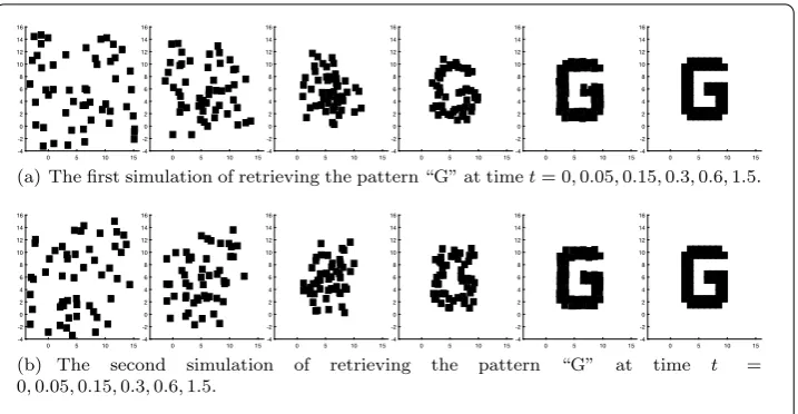
Figure 4Two simulations of retrieving the pattern “G” with random initial values
follows:
J= (–7.3442 + 17.2369i, –5.2027 + 29.3254i, . . . , 21.8742 + 33.4738i)T. (44)
Here we just list some of the elements ofzˇandJdue to space limitations. Two simula-tions with random initial values depicted in Fig. 4 show that the designed CVNNs with parameters (40)–(44) have the ability of recalling the above pattern “G” reliably.
Next, we take use of the above neural network with the same parameters (40)–(43) to memorize another image pattern “A”. However, the parameterJ should be recomputed since the positions of the black block in image pattern “A” are different from those in image pattern “G”. Noting that the pattern “A” composed of 50 black blocks, we should add 2 additional block such that there are 52 blocks. Then the equilibrium pointzˇis designed as
ˇ
z= (2 + i, 2 + 2i, . . . , –10 – 10i, –10 – 10i)T∈C52,
where the first 50 elements ofˇzcorrespond the 50 coordinates of the black block in image pattern “A”, and the last two elements are additional. According to the equilibrium point
ˇ
z, the external inputsJcan be computed as follows:
J= (–6.2332 + 8.3721i, –4.0371 + 19.3896i, . . . , –62.0099 – 46.0415i)T. (45)
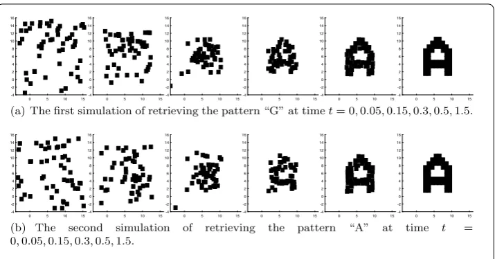
Two simulations with random initial values depicted in Fig. 5 show that the designed CVNNs with parameters (40)–(43) and (45) have the ability of recalling the above pat-tern “A” reliably.
Remark6 In Example 2, since the neurons are complex-valued, each neuron contains the horizontal and vertical coordinates of the black blocks in the images. Thus the designed CVNNs require less neurons than RVNNs to store the image patterns.
6 Conclusion
Figure 5Two simulations of retrieving the pattern “A” with random initial values
complex domain, we presented some sufficient conditions to guarantee the existence of a unique equilibrium point for the complex-valued neural networks. In addition, by con-structing appropriate Lyapunov–Krasovskii functionals, and employing the matrix in-equality techniques, we obtained several conditions for checking the robust stability of the complex-valued neural networks which are established in LMIs. Finally, two numer-ical examples have been given to illustrate the effectiveness of the proposed theoretnumer-ical results.
Funding
This work was supported in part by the National Natural Science Foundation of China under Grant 11471201, in part by the Program of Chongqing Innovation Team Project in University under Grant CXTDX201601022, in part by the Natural Science Foundation of Chongqing Municipal Education Commission under Grant KJ1705138, and in part by the Natural Science Foundation of Chongqing under Grant cstc2017jcyjAX0082.
Competing interests
The authors declare that they have no competing interests.
Authors’ contributions
All authors conceived of the study, participated in its design and coordination, read and approved the final manuscript.
Author details
1College of Mathematics and Statistics, Chongqing Jiaotong University, Chongqing, China.2School of Mathematics and
Statistics, Shaanxi Normal University, Shaanxi, China.
Publisher’s Note
Springer Nature remains neutral with regard to jurisdictional claims in published maps and institutional affiliations.
Received: 4 December 2017 Accepted: 9 February 2018 References
1. Hirose, A.: Complex-Valued Neural Networks: Theories and Applications. World Scientific, Singapore (2004) 2. Rao, V.S.H., Murthy, G.R.: Global dynamics of a class of complex valued neural networks. Int. J. Neural Syst.18(2),
165–171 (2008)
3. Tanaka, G., Aihara, K.: Complex-valued multistate associative memory with nonlinear multilevel functions for gray-level image reconstruction. IEEE Trans. Neural Netw.20, 1463–1473 (2009)
4. Zeng, Z., Zheng, W.X.: Multistability of neural networks with time-varying delays and concave-convex characteristics. IEEE Trans. Neural Netw. Learn. Syst.23(2), 293–305 (2012)
5. Yang, R., Wu, B., Liu, Y.: A Halanay-type inequality approach to the stability analysis of discrete-time neural networks with delays. Appl. Math. Comput.265, 696–707 (2015)
7. Rakkiyappan, R., Sivaranjani, R., Velmurugan, G., Cao, J.: Analysis of globalO(t–α) stability and global asymptotical
periodicity for a class of fractional-order complex-valued neural networks with time varying delays. Neural Netw.77, 51–69 (2016)
8. Liu, Y., Xu, P., Lu, J., Liang, J.: Global stability of Clifford-valued recurrent neural networks with time delays. Nonlinear Dyn.84(2), 767–777 (2016)
9. Chen, X., Song, Q., Liu, X., Zhao, Z.: Globalμ-stability of complex-valued neural networks with unbounded time-varying delays. Abstr. Appl. Anal.2014, Article ID 263847 (2014)
10. Gong, W., Liang, J., Cao, J.: Globalμ-stability of complex-valued delayed neural networks with leakage delay. Neurocomputing168, 135–144 (2015)
11. Tu, Z., Cao, J., Alsaedi, A., Alsaadi, F.E., Hayat, T.: Global Lagrange stability of complex-valued neural networks of neutral type with time-varying delays. Complexity21(S2), 438–450 (2016)
12. Shao, J., Huang, T., Wang, X.: Further analysis on global robust exponential stability of neuural networks with time-varying delays. Commun. Nonlinear Sci. Numer. Simul.17, 1117–1124 (2012)
13. Shi, Y., Cao, J., Chen, G.: Exponential stability of complex-valued memristor-based neural networks with time-varying delays. Appl. Math. Comput.313, 222–234 (2017)
14. Senan, S.: Robustness analysis of uncertain dynamical neural networks with multiple time delays. Neural Netw.70, 53–60 (2015)
15. Zhang, W., Li, C., Huang, T.: Global robust stability of complex-valued recurrent neural networks with time-delays and uncertainties. Int. J. Biomath.7, 79–102 (2014)
16. Samli, R.: A new delay-independent condition for global robust stability of neural networks with time delays. Neural Netw.66, 131–137 (2015)
17. Feng, W., Yang, S., Wu, H.: Further results on robust stability of bidirectional associative memory neural networks with norm-bounded uncertainties. Neurocomputing148, 535–543 (2015)
18. Chen, H., Zhong, S., Shao, J.: Exponential stability criterion for interval neural networks with discrete and distributed delays. Appl. Math. Comput.250, 121–130 (2015)
19. Li, Q., Zhou, Y., Qin, S., Liu, Y.: Global robust exponential stability of complex-valued Cohen–Grossberg neural networks with mixed delays. In: 2016 Sixth International Conference on Information Science and Technology (ICIST), pp. 333–340. IEEE (2016)
20. Bainov, D., Simenov, P.: System with Impulsive Effect: Stability, Theory and Applications. Wiley, New York (1989) 21. Tang, S., Chen, L.: Density-dependent birth rate, birth pulses and their population dynamic consequences. J. Math.
Biol.44, 185–199 (2002)
22. Song, Q., Yan, H., Zhao, Z., Liu, Y.: Global exponential stability of complex-valued neural networks with both time-varying delays and impulsive effects. Neural Netw.79, 108–116 (2016)
23. Chen, X., Li, Z., Song, Q., Hu, J., Tan, Y.: Robust stability analysis of quaternion-valued neural networks with time delays and parameter uncertainties. Neural Netw.91, 55–65 (2017)
24. Zhang, X., Li, C., Huang, T.: Impacts of state-dependent impulses on the stability of switching Cohen–Grossberg neural networks. Adv. Differ. Equ.2017(1), 316 (2017)
25. Wan, L., Wu, A.: Mittag-Leffler stability analysis of fractional-order fuzzy Cohen–Grossberg neural networks with deviating argument. Adv. Differ. Equ.2017(1), 308 (2017)
26. Zhu, Q., Cao, J.: Stability analysis of Markovian jump stochastic BAM neural networks with impulsive control and mixed time delays. IEEE Trans. Neural Netw. Learn. Syst.23, 467–479 (2012)
27. Hu, J., Wang, J.: Global stability of complex-valued recurrent neural networks with time-delays. IEEE Trans. Neural Netw. Learn. Syst.23, 853–865 (2012)
28. Zhang, Z., Lin, C., Chen, B.: Global stability criterion for delayed complex-valued recurrent neural networks. IEEE Trans. Neural Netw. Learn. Syst.25, 1704–1708 (2014)
29. Chen, X., Song, Q.: Global stability of complex-valued neural networks with both leakage time delay and discrete time delay on time scales. Neurocomputing121, 254–264 (2013)
30. Song, Q., Yan, H., Zhao, Z., Liu, Y.: Global exponential stability of impulsive complex-valued neural networks with both asynchronous time-varying and continuously distributed delays. Neural Netw.81, 1–10 (2016)
31. Rao, V., Murthy, G.: Global dynamics of a class of complex valued neural networks. Int. J. Neural Syst.18, 165–171 (2008)
32. Bohner, M., Rao, V., Sanyal, S.: Global stability of complex-valued neural networks on time scales. Differ. Equ. Dyn. Syst. 19, 3–11 (2011)
33. Nitta, T.: Orthogonality of decision boundaries of complex-valued neural networks. Neural Comput.16, 73–97 (1989) 34. Amin, M., Murase, K.: Single-layered complex-valued neural network for real-valued classification problems.
Neurocomputing72, 945–955 (2009)
35. Hirose, A.: Complex-Valued Neural Networks: Theories and Applications. World Scientific, Singapore (2004) 36. Huang, C., Cao, J., Xiao, M., Alsaedi, A., Hayat, T.: Bifurcations in a delayed fractional complex-valued neural network.
Appl. Math. Comput.292, 210–227 (2017)
37. Rakkiyappan, R., Udhayakumar, K., Velmurugan, G., Cao, J., Alsaedi, A.: Stability and Hopf bifurcation analysis of fractional-order complex-valued neural networks with time delays. Adv. Differ. Equ.2017(1), 225 (2017) 38. Tan, Y., Tang, S., Yang, J., Liu, Z.: Robust stability analysis of impulsive complex-valued neural networks with time
delays and parameter uncertainties. J. Inequal. Appl.2017, 215 (2017)
39. Chen, X., Song, Q., Liu, Y., Zhao, Z.: Globalμ-stability of impulsive complex-valued neural networks with leakage delay and mixed delays. Abstr. Appl. Anal.2014, Article ID 397532 (2014)
40. Zou, B., Song, Q.: Boundedness and complete stability of complex-valued neural networks with time delay. IEEE Trans. Neural Netw. Learn. Syst.24, 1227–1238 (2013)