J. Imaging 2019, 5, x; doi: FOR PEER REVIEW www.mdpi.com/journal/jimaging
Teleporting digital images
Mario Mastriani
Quantum Communications Lab, Qubit Reset LLC, 2875 NE 191, suite 801, Aventura, FL 33180, USA [email protected]
https://www.qubitreset.com http://orcid.org/0000-0002-5627-3935
Abstract: During the last 25 years the scientific community has coexisted with the most fascinating
protocol due to Quantum Physics: quantum teleportation (QTele), which would have been impossible if quantum entanglement, so questioned by Einstein, did not exist. In this work, a complete architecture for the teleportation of Computational Basis States (CBS) is presented. Such CBS will represent each of the possible 24 classical bits commonly used to encode every pixel of a 3-color-channel-image (red-green-blue, or cyan-yellow-magenta). For this purpose, a couple of interfaces: classical-to-quantum (Cl2Qu) and quantum-to-classical (Qu2Cl) are presented with two versions of the teleportation protocol: standard and simplified.
Keywords: Interfaces; Quantum Communications; Quantum Entanglement; Quantum Image
Processing; Quantum Teleportation; Superdense Coding.
1. Introduction
1.1 Quantum Teleportation
In 1993 a fundamental paper for the history of Physics was published [1], where a protocol for the teleportation of an unknown quantum state was proposed without violating the No-Cloning Theorem [2]. This protocol uses a strange phenomenon of Quantum Mechanics (QMech) known as Quantum Entanglement (QEnta), in which two or more particles leave their individualities to become part of something unique and integral. These particles retain the aforementioned attribute even if they are separated to opposite places in the universe.
Now, if we measure one of those particles, the entanglement disappears, the joint wave function collapses, and if the measured particle becomes a spin-up, the other instantaneously becomes a spin-down, and vice-versa. This instantaneity is given independently of the distance that mediates between both particles, contradicting the very essence of Special Relativity (SRela) [3], which postulates that nothing can travel faster than light. This curious result was called by Einstein as "spooky action at a distance", and constitutes the center of one of the most famous paradoxes in the history of Physics suggested by Albert Einstein, Boris Podolsky and Nathan Rosen known as EPR paradox [4]. There is a palliative to this controversy which consists in the impossibility of transmitting useful information through an instantaneous link based on entanglement [1]. This palliative constitutes a hot border between two of the main pillars of Physics: the SRela [3] and QMech [5].
In 1964 John Bell [6] tried to solve this controversy by proposing a theorem based on an inequality by which the non-locality of QMech could be established as long as it violated such inequality. Experiments carried out by Aspec [7-9] and others (with and without loop-holes) apparently established the non-locality of QMech, contradicting what was manifested by the EPR paradox. Part of the scientific community does not question the non-locality of QMech, since there is an absolute consensus, however, they are hesitant about the quality of the mentioned experiments.
Since 1997, a series of experiments have demonstrated the practical feasibility of QTele protocol (QTele) [10-18], even in the presence of noise [19-22]. Thirteen years later, Prof. Hotta [23] demonstrated how energy could be teleported, triggering all kinds of speculations about the possible teleportation of matter, by virtue of the close link between matter and energy starting from the famous Einstein equation, E = m c2, for a particle at rest. Currently, a simplified version of the original QTele protocol [24, 25] opens up a whole new range of possibilities in Quantum Communications (QComm) [26-29] thus completing the arsenal of essential tools for Quantum Technology to be used in the future.
1.2 Superdense Coding
A complementary protocol to the QTele, called Superdense Coding (SDC) [1], allows us to send classical bits through a quantum channel. Besides, SDC is the foundational basis of a couple of interfaces needed when handling CBS in a QComm context [27]. Recently, a new SDC protocol based on a simplified version of QTele has come out with remarkable results [25]. In fact, the mentioned protocol is presented as the most probable basis for secure communication between Earth and Mars, in a future mission to Mars.
1.3 Interfaces
The need for Cl2Qu and Qu2Cl interfaces in all branches of Quantum Information Processing (QIP) is evident [30], however, in no other case as in Quantum Image Processing (QImP) has it become so evident. Works like Quantum Boolean Image Denoising [31] highlight the imperative need for an efficient interface between each of the possible 24 classical bits commonly used to encode each pixel of an image with 3 color channels (red, green, blue) and the internal representation that said classical bits must have within the quantum computer, that is, as CBS. This conversion cannot result from a qubits preparation procedure because the images are too large, this must be done automatically thanks to an interface. For example, for an image of 1920 columns, 1080 rows, 8 bits-by-color, and 3 colors (an image of common size these days), we must prepare 49,766,400 qubits (in this particular case: CBS). This is highly impractical, since, how long would a similar amount of qubit preparations take us in a laboratory? The problem of Quantum Measurement (QuMe) [32] has confined the practicality of QImP to the exclusive use of CBS, as it is exposed in [33]. If we wanted to work in QImP with generic qubits, we would find ourselves with a problem that does not exist to date even with Cl2Qu interface for this type of qubit. Besides, it is impossible to recover exactly the Quantum Algorithm (QAlgo) result because of QuMe [32], as explained in [33]. It happens that the measurement noise due to QuMe is greater than that admissible in a standard process of Digital Image Processing (DIP) [34-37]. The distortion in the recovery of a qubit at the output of a QAlgo is greater than that normally accepted [33], being the Heisenberg Uncertainty Principle (HUP) and the complementarity [30], the exclusive responsible for it, as explained in [33]. This is the problem that fundamentally affects the internal representation technique known as Flexible Representation of Quantum Images (FRQI) [38] and all its variants. Besides, another famous technique within QImP is that known as Novel Enhanced Quantum Representation (NEQR) [39]. The problem with NEQR, as well as all its variants, is that it is not a Cl2Qu Interface, however, they need one. In fact, if we had a Cl2Qu interface, then why would we need NEQR? On the other hand, the reason why both techniques (FRQI and NEQR) are accepted within QImP resides in the fact that all the papers that mention them only involve implementations in a high-level interpreter such as MATLAB® [40], and not on an optical table as it should be. Under these circumstances everything seems to work, but when done on an optical table the real outcome is very different.
2. Materials and Methods
2.1 A brief of Quantum Information Processing
1
0
, (1)
where is called wave function, and are complex numbers such that 2 2 1, and
the states 0
1 0
T and 1
0 1
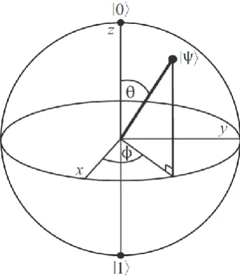
T (being [•]T the transpose of [•]) are understood asdifferent polarization states of light allocated at the poles of the Bloch’s sphere (Figure 1).
Figure 1. Bloch’s Sphere.
These states
0 ,1
constitute an orthonormal basis and they are known as CBS and can beexpressed in several ways:
Spin up = = 0 = 1 0
= 0 qubit basis state = North Pole (2)
and
Spin down = =1 = 0 1
= 1 qubit basis state = South Pole (3)
On the other hand, a more general analysis of the wave function allows us to establish that
0 1 0 1
2 2 2 2
i i i
ecos e sin ecos cos i sin sin
(4)
where 0 , 0 2 . We can ignore i
e from Equation (4), because it has no observable effects [30], therefore, we can effectively write:
0 1
2 2
i
cos e sin
The angles and define a point on the unit three-dimensional sphere (Figure 1), with,
2 2
i
cos, e sin
(6)
Except in the case where is one of the CBS 0 or 1 , in all other cases, the representation
needs to use the superposition principle [30]. The parameters and can be re-interpreted as spherical coordinates specifying a point
x y z
a a ,a ,a sin cos , sin sin , cos (7)
on the unit sphere in 3 (according to Equation 4). In other words, the state of a qubit is a unit
vector in the two-dimensional complex Hilbert’s space 2. Finally, a column vector is called a
ket vector
T, while a row vector is called a bra vector * *
, where, (•)* means
complex conjugate of (•).
2.2 Color decomposition and bit slicing
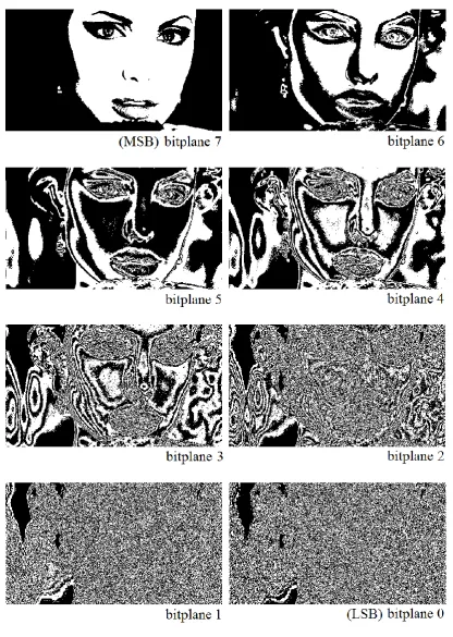
First, we need to decompose all digital images in their 3 color components (red, green, blue) [31]. Thus, we will obtain 24 bitplanes (8 bitplanes for every color) thanks to a procedure known as bit slicing [31]. We get 8 bitplanes per color, where the 7th bitplane (the closest to the observer) is called the Most Significant Bit (MSB) being the most morphologically committed bitplane with the original image [31] (Figure 2). Conversely, bitplane 0 (the furthest from the observer) is the Least Significant Bit (LSB) and the least morphologically committed bitplane with the original image. Below, we provide the MATLAB® code [40] necessary for slicing:
function Ibpp = slicer(I,bpp)
% Casting of the algorithm:
% bpp = bit-per-pixel
% I = Each color component of the image
% Ibpp = I in bpp bitplanes (strictly binary)
[ROW,COL] = size(I);
for r = 1:ROW
for c = 1:COL
aux = d2b(I(r,c)-1,bpp);
for b = 1:bpp
Ibpp(r,c,b) = aux(b);
end
end
end
return;
function bvpp = d2b(p,bpp)
% Casting of algorithm:
% d = bit depth
% p = pixel value
% bvpp = binary vector per pixel
bvpp = zeros(1,bpp);
d = 1;
while p > 0,
bvpp(d) = mod(p,2);
p = p/2;
p = floor(p);
d = d+1;
end
bvpp = rot90(rot90(bvpp));
Figure 2. Bitplanes of the red component for Angelina obtained by slicing, with special remarks for
MSB and LSB.
It is evident, from here on, that an element in black in every bitplane is a classical bit equal to 1
and will be represented with a qubit equal to
1
, while, an element in white in every bitplane is aFigure 3. Angelina and her 8 bitplanes, including MSB and LSB.
2.3 Standard Quantum Teleportation - noiseless analysis
QTele begins with the distribution of an EPR pair between Alice and Bob. We can choose any of the EPR of the complete set of Bell’s basis:
00 01
10 11
1 1
00 11 00 11
2 2
1 1
01 10 01 10
2 2
,
,
(8)
We normally choose
00 . This distribution constitutes the entanglement link between Aliceand Bob. After that, we continue with the complete sketch of QTele of Figure 4, where the green line indicates the border between Alice’s and Bob’s sides, that is, both extremes of the entanglement link. In Figure 4, a single fine line represents a wire carrying one qubit, while a double line represents a wire carrying one classical bit [30], while, the classical channel is really a control classical channel for disambiguation purposes (as we will see below through two bits), while the entanglement link is really an entanglement data link. On the other hand, in Figure 4, the following blocks mean: SPD (single photon detectors), {x , z} are Pauli’s matrices activated by the bits {b2, b1} respectively [1, 30],
and EPR is the source of
00
A B of Equation (8).Figure 4. Standard teleportation protocol using an EPR pair and two classical bits for
disambiguation.
Now, If 0 0 1 is an arbitrary and unknown state to be teleported with
2 2
1
and
of a Hilbert’s space, then, the initial state (3-partite state) will be,
0 00 00 0 1 1 2 00 11
1 0 00 11 1 00 11 1 000 011 100 111
2 2
0 0 0 0
2 2 2 2
T
(9)
where for simplicity (and from here on) we have adopted
x
y
x y
in a generic form, andNow, a CNOT gate is applied to Equation (9),
1
1
000 011 110 101
2
0 0 0 0
2 2 2 2
T
(10)
In practice, Kronecker’s product and CNOT gate are implemented together on the same beamsplitter [10, 11, 16-18]. Then, we apply a Hadamard’s gate to the elements of Equation (10),
0 0 1 0 0 1 1 1
2
0 0 1 0 0 1 1 1
0 0
0 1
1
00 01 10 11
2 1 2
2 2 2 2 2 2 2 2
0 0 0 0 0 0 00 00
2 2
0 0 0 0 0 0 10 10
2 2
0 0 0 0 0 0
2 2
x z x z x z x z
x z x z x z x z
T T x z T x z
1 0
1 1
01 01
0 0 0 0 0 2 0 2 11 11
T x z T x z (11)
The last rows of Equation (11) represent Alice’s options inside the SPD. Alice randomly selects one of the bases and performs the measurement, transmitting to Bob the corresponding classical bits through a classical channel. Alice's options within the SPD are equally probable and the random choice that she makes of the base has to do with being sure not to clone the original state between her and Bob [10, 11].
Table 1 synthesizes the complete process of QTele, where Alice measures two of the possible qubits of the basis of Equation (8), and therefore, she transmits the corresponding bits b1 and b2 via a
classical channel to Bob. The QMeas process is imperative to make the wave-function of the original arbitrary state collapse since this is necessary to do so as not to violate the No-Cloning Theorem [2]. In other words, the QMeas process destroys the original arbitrary state [30, 32] eliminating any possibility of cloning.
Table 1. Alice’s side: measurement of the base, classical transmission of bits, and the collapse of states,
Bob’s side: classical reception of bits, gates application for the final recovery of the arbitrary state.
Alice’s measurement
Alice transmits
This happens with
probability Collapsed state Bob applies
1 2 b b x z 00
b2 b1 = 00
2
0 0
1 1
2
x z
40 0
x z
0 0
x z
01
b2 b1 = 012
1 0
1 1
2 x z 4
1 0
x z
1 0
x z x
10
b2 b1 = 102
0 1
1 1
2
x z
40 1
x z
0 1
x z z
11
b2 b1 = 112
1 1
1 1
2
x z
41 1
x z
1 1
x z x z
The last column of Table 1 represents the local operations realized by Bob in t3 and t4 to
reconstruct the original state
. At this point, it is important to mention that in literature there are several concerns regarding the implementation of teleportation protocols using a bigger or smaller dimensional commitment but always with two classical bits for disambiguation. An interesting example can be found in [42], which shows that the one-qubit teleportation can be considered as a state transfer between subspaces of the whole Hilbert’s space of an indivisible eight-dimensional system. However, this as well as the rest of the papers that manipulate high dimensional quantum systems for the implementation of QTele protocols do it with two classical bits for disambiguation, except in the case of the new protocol presented here which does not use disambiguation bits.On Alice's side, the combination of the modules composed by the following gates: CNOT, H (Hadamard) and QMeas, constitute what is known as the Bell-State-Measurement (BSM), while on Bob's side, its modules are unitary operations necessary for the reconstruction of the teleported state. Alice’s measurement and transmission of the classical bits of disambiguation along with Bob's unitary operations are the clearest examples of Local Operations and Classical Communications (LOCC) [43].
2.4 Standard Quantum Teleportation - noisy analysis
Starting again from Figure 4, and considering noise in the EPR pair by a disturbance of the shape
00 n A00 B11
(12)
where subscript n means noise, and
2 2
1
A
B
, with
1
1
2 2
A
B
A
B
(13)Then, repeating Equation (9) but with 00
n
instead of 00 , we will have
0 00 0 1 00 11
000 100 011 111
n A B
A A B B
(14)
Now, a CNOT gate is applied to Equation (14), resulting in
1 A000 A110 B 011 B101
. (15)
Then, we apply a Hadamard’s gate to the elements of Equation (15),
2 1
000 100 010 110 011 111 001 101
2
00 0 00 1 10 0 10 1 01 0 01 1 11 1 11 0
2 2 2 2 2 2 2 2
1
00 0 1 10 0 1 01 1 0 11 1 0
2
A A A A B B B B
A B A B A B B A
A B A B B A B A
From here on, we will follow a procedure similar to that of Table 1 but taking into account how sensitively the state is affected by noise. In fact, seeing Equation (16), it is evident that it is almost impossible to recover the state in an exact way [19-22, 24, 25].
2.5 Simplified Quantum Teleportation - noiseless analysis
Unlike the standard version, the new protocol frees us from the use of a classical channel to transmit the disambiguation bits, and the use of Pauli’s matrices in Bob's side used to reconstruct the teleported state from the mentioned disambiguation bits. These simplifications are the underlying reasons for the title of this paper, that is, simplified protocol.
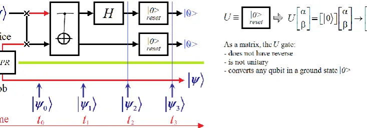
In the new protocol (Figure 5), block “
0
reset” does a strict reset of the qubit, while, we need to produce 00 instead of 00 used in the standard version. We must highlight as a fundamental contrast between both versions of QTele (the standard and the simplified) that the Kronecker product “
” is not commutative [30].Figure 5. Simplified teleportation protocol using an EPR pair but without classical bits for disambiguation.
0 00
1
00 11 0 1
2 1
000 001 110 111
2
0 0 0 0
2 2 2 2
T
(17)
Now, a CNOT gate is applied to Equation (17), and the result will be present on the Alice’s
lower branch, because in her upper branch will be
00 ,
1
1 1
000 001 100 101 00 0 1 10 0 1
2 2
1 1
0 1 00 10 0 1 0 1 0 0
2 2
(18)
Figure 5 shows that the Hadamard’s gate only involves to the Alice’s upper branch, then,
00
1 0 1 1 1 1
00 11
0 1 2 1 1 2
1
00 10 01 11
2
IH
It is clear from Equation (18) that no disambiguation is necessary. Alice blocks her two branch thanks to a qubit reset gate [|0>] pair in order to annul all the projections with |1> components in Eq.(18) and (19). The No-Cloning Theorem [2] is never violated. We can also see in Figure 5 that it is not necessary for Bob to apply any unitary transformation. This eliminates the classical channel that is responsible for making teleportation as a whole to be carried out in a time greater than zero, i.e., not being instantaneous.
Although this result seems to contradict the relativistic principle of causality [4], the reality is that this never happens. As we can see in [25], the instantaneity of entanglement is possible without the need to resort to superluminal signaling and without any contradictions between QMech and SRela. This last fact then covers the new protocol in a direct and complete way.
2.6 Simplified Quantum Teleportation - noisy analysis
For noisy EPR pairs we also resorted to Figure 5 using the same version of Equations (12) and (13). Then, repeating Equation (17) but with 00
n
instead of 00 , we will have
0 00 00 11 0 1
000 110 001 111
n A B
A B A B
(20)
Now, we apply a CNOT gate to Equation (20), and the result will be present on the Alice’s lower
branch again, because in her upper branch will be
00 ,
1 000 100 001 101
00 0 1 10 0 1
00 10 0 1
00 10
A B A B
A B A B A B C (21) where,
00 10
C A B (22)
In this case again, the Hadamard’s gate only involves to the Alice’s upper branch, then,
00
1 0 1 1 1
00 11
0 1 2 1 1
1
00 10 01 11
2 n
I H A B
A A B B
(23)
2.7 Interfaces
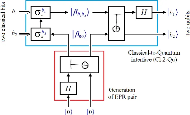
From SDC emerges an extraordinary set of interfaces for an efficient relationship between classical bits and CBS, and vice-versa. Figure 6 shows the SDC protocol, which is composed of two well-defined blocks: one which is light blue and the other one pink. The light blue block works as a Cl2Qu interface, while the pink block works as a Qu2Cl interface. All this, of course, is exclusively defined to be used with classical bits, and in consequence, CBS.
Figure 6. SDC protocol and the detail of its constituent interfaces.
Next, we will describe how the SDC protocol works from left to right, which is the correct way of describing how both interfaces (Cl2Qu and Qu2Cl) work. An important detail to highlight before starting is that we can work with: 2 classic bits to be transmitted (Figure 6), a single classic bit (b1) to
be transmitted and b2 which makes ancilla equal to zero, or N classic bits to be transmitted as a
natural extension of the protocol of Figure 6. This last case will be particularly useful in the practical application of the interfaces for the treatment of digital images, in such a way that N = 24 and each application of the protocol implies working with a complete pixel of a color image. For a better development of the idea, we will work with 2 classic bits extracting Cl2Qu from Figure 6 to form Figure 7.
We begin with both possibilities according to b2, i.e., 0 or 1. If b2 = 0, then, in t1 we will have
00
again (Figure 6). But, if b2 = 1, then, in t1 we will have,
1 1 2 2 1 2 00 1 2 1 1 2 20
0
1
0
0
0
0
0
1
1
0
0
0
0
1
0
0
1
0
0
1
1
0
0
0
0
1
0
0
0
x
I
(24)If in t2, b2 = 0 and b1 = 0, we will obtain
00 . But if b2 = 0 and b1 = 1, we will have,
1 1 1
2 2 2
00
1 1 1
2 2 2
1
0
0
0
0
0
0
1
0
1
0
0
1
0
0
0
0
0
0
1
0
1
0
0
1
0
0
0
0
1
z
I
(25)Now, if b2 = 1 and b1 = 1, we will use the result of Equation (24) to obtain the state in t2,
1 2 1 2 1 2 1 21 1 1 1
2 2 2 2
0
0
1
0
0
0
0
0
1
0
1
0
0
1
0
0
0
1
0
1
0
0
1
0
0
0
0
0
0
1
0
0
z
I
(26)Obviously, the result in t2 is the same as in t3 (Figure 6). The four obtained results, according to
the values of b2 and b1, travel through the optical channel of Figure 6 under the generic name of
1 2
b b
.Now, if we apply CNOT gate to these results, then, for b2 = 0 and b1 = 0, we will have,
1 1 2 2 1 2 1 2
1
0
0
0
0
0
1
0
0
0
0
0
0
0
1
0
0
1
0
0
(27)For b2 = 0 and b1 = 1,
1 1 2 2 1 2 1 2
1
0
0
0
0
0
1
0
0
0
0
0
0
0
1
0
0
1
0
0
For b2 = 1 and b1 = 0, 1 1 2 2 1 2 1 2
0
1
0
0
0
0
0
1
0
0
0
0
0
0
1
0
0
1
0
0
(29)For b2 = 1 and b1 = 1,
1 1 2 2 1 2 1 2
0
1
0
0
0
0
0
1
0
0
0
0
0
0
1
0
0
1
0
0
(30)At this point, it is important to clarify that the quantum channel of Figure 6 inside the Cl2Qu interface is obviously unnecessary (Figure 7). In fact, the definitive Cl2Qu interface is absolutely compact and henceforth it will be considered as a unified block. Finally, we will apply the Hadamard’s gate to the last set of equations according to Figures 6 and 7 [24, 25], thus,
for b2 = 0 and b1 = 0, we will have,
1 1
1 1 1
2 2
2 2 2
1 1 1 1
2 2 2 2
1 1 1 1
1 1 1
2 2 2 2
2 2 2
1 1
2 2
0
0
0
0
0
1
0
0
0
0
0
0
1
0
0
0
0
0
1
0
1
1
0
0
00
0
0
0
0
H
I
(31)for b2 = 0 and b1 = 1,
1 1
1 1 1
2 2
2 2 2
1 1 1 1
2 2 2 2
1 1 1 1
1 1 1
2 2 2 2
2 2 2
1 1
2 2
0
0
0
0
0
1
0
0
0
0
0
0
1
0
0
0
0
0
0
0
0
1
1
0
10
1
1
0
0
H
I
(32)
1 1
2 2
1 1 1 1 1 1 1
2 2 2 2 2 2 2
1 1 1 1
2 2 2 2
1 1 1 1 1
2 2 2 2 2
0
0
0
0
0
0
0
1
0
0
0
1
0
0
0
0
0
0
0
1
1
0
0
1
01
0
0
1
0
H
I
(33)for b2 = 1 and b1 = 1,
1 1
2 2
1 1 1 1 1 1 1
2 2 2 2 2 2 2
1 1 1 1
2 2 2 2
1 1 1 1 1
2 2 2 2 2
0
0
0
0
0
0
0
1
0
0
0
1
0
0
0
0
0
0
0
0
0
0
1
1
11
0
1
1
1
H
I
(34)Here Cl2Qu interface finalizes. Basically, Cl2Qu interface is a block that performs a transfer of type
b b1, 2
b1 ,b2
for CBS, i.e.,
0,1
0 , 1
.The pink block of Figure 6 constitutes the Qu2Cl interface. In fact, at the entrance of that block, we have
b1 , b2
, while at its exit we have
b b
1,
2
, i.e., QuMe is a Qu2Cl interface in itself. With this sequence Cl2Qu + Qu2Cl we complete the standard SDC. In this way, the circle closes, and at least in theory, we should recover at the exit of the pink block the same classical bits that we have entered at the entrance of the light blue block. Consequently, we can use a coincidence counter to evaluate the performance of the complete SDC protocol, and to know what the level of coupling between both interfaces is.A relevant detail to take into account is that when we measure a CBS, we completely recover its classical counterpart, a situation very different from what happens with a generic qubit, which does not have a classical counterpart and if it existed it would be unattainable to obtain it [30, 31, 33]. In fact, it is only necessary to make a measurement on the z-axis of the Bloch’s sphere (vertical) avoiding the typical problems associated with QuMe, HUP and reciprocity [30-33].
2.8 Complete architecture to be used
Figure 8 represents a complete architecture for an enhanced SDC. This figure shows both interfaces where we can appreciate a pair of green blocks labeled QTele between them. Actually, these blocks can represent the two types of seen teleportations: standard and simplified. Besides, these blocks constitute the imaginary boundary between Alice’s and Bob’s sides. It is important to mention that this configuration can be used to transmit a single classic bit at a time, where, b2 could
Figure 8. Enhanced SDC using Cl2Qu and Qu2Cl interfaces and two blocks of QTele.
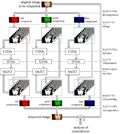
If we expand the idea of Figure 8 by involving the steps necessary to decompose a color digital image in their corresponding constituent bits, then, we will arrive to Figure 9. This is essentially the scheme we will use for the experiments in the next section. Figure 9 shows on top the original image to be teleported, then the three color channels (red, green and blue) of the image are separated. Later, each color channel is decomposed in 8 bitplanes. The bit of each bitplane is introduced into a Cl2Qu interface. The equivalent qubits are teleported. Bob receives each qubit with a Qu2Cl interface. With the obtained bits, the bitplanes are reconstructed, then the three color channels are reassembled and
finally the teleported image is obtained. The lower part of Figure 9 shows a comparison between the acquired bit of the original image and the recovered bit from the complete architecture.Finally, the complete comparison of all individual bits becomes the total comparison between both images: the original and the teleported one for the purpose of evaluating the level of degradation introduced by the complete procedure usingas a metric the coincidence counter. Notwithstanding the foregoing, in the following section, the intermediate instances of each step of the procedure will also be monitored and analyzed.
3. Results
3.1. Setup
All experiments of this section consist of implementations on Quirk® [44] simulator. In the complete architecture for the QTele of Angelina image (Figure 9), we randomly select 100 of the 1920x1080x3x8 bits of the original image, although fewer bits of alternate values (i.e., 0 and 1) and from different locations would be enough.
We will evaluate the performance in the reconstruction of such bits thanks to a coincidence counter, which can be seen in the lower part of Figure 9.
Finally, we will clarify the number of qubits used in each simulation carried out with the Quirk® simulator, as well as the corresponding circuit lay-out, in order to facilitate the reproduction of all the experiments done here.
3.2. Partial tests
These experiments involve evaluating separately each of the protocols to be used in the final configuration for the QTele of the image, before proceeding with it. Such experiments aim to unmask in an individual way the possible responsible for the collectively incorrect results.
3.2.1. Superdense coding
Based on the protocol of Figure 6, we will implement the complete SDC, which is equivalent to the union between Cl2Qu and Qu2Cl interfaces. Figure 10 represents the complete configuration for Quirk® simulator with the explicit results inside the figure through a series of activation (on) and deactivation (off) flags, from {b1,b2}={0,0} to {b1,b2}={1,1}.
Figure 10(a). SDC
Cl2Qu
Qu2Cl on Quirk® for {b1,b2}={0,0}.Figure 10(c). SDC
Cl2Qu
Qu2Cl on Quirk® for {b1,b2}={0,1}.Figure 10(d). SDC
Cl2Qu
Qu2Cl on Quirk® for {b1,b2}={1,1}.For this experiment, we used 4 qubits on the Quirk® simulator. The total coincidences of the flags (in on or off, at the entrance and exit of the protocol) in the four cases (i.e., 00, 01, 10 and 11) represent the success in the SDC process. The connection labelled as send represents the optical channel in yellow in Figure 6, although, as it is obvious, within the Cl2Qu interface such a connection does not exist. Finally, 3 points in a row represent the border between both blocks.
The experimental implementation for the transmission of 100 classical bits taken into pairs and their posterior recovering gave us as a result on Quirk® simulator a complete set of coincidences. It is evident that fewer pairs would have given the same results.
3.2.2. Standard QTele
Figure 11 shows the complete process of Standard QTele, which is only implemented thanks to 3 qubits on Quirk® simulator.
Figure 11(a) remits us to the case of a generic qubit, which has an arbitrary allocation on the Bloch’s sphere [30]. Figures 11(b) and 11(c) show a pair of particular cases where the qubits are both CBS, i.e., 0 and 1, respectively.
As in the case of Figures 4 and 5, a single fine line represents a wire carrying one qubit, while a double line represents a wire carrying one classical bit [30].
The possibility of a fast, precise and graphically expressive simulation on a complete toolbox environment, independently of the pertinent code makes Quirk® simulator an attractive choice.
Figure 11(b). Standard QTele for the teleportation of 0 .
Figure 11(c). Standard QTele for the teleportation of 1 .
3.2.3. Simplified QTele
Figure 12 shows the Simplified QTele with identical considerations to the previous case.
Figure 12(a). Simplified QTele for a generic qubit to be teleported.
Figure 12(b). Simplified QTele for the teleportation of 0 .
3.3. Standard QTele of a digital image
As we have said, this is the first implementation for the QTele of an image. Figure 13 represents such implementation on Quirk® simulator.
The architecture of Figure 13 shows the perfect complementation between the Standard QTele and both interfaces, i.e., Cl2Qu and Qu2Cl. This configuration required 8 qubits.
We must bear in mind that at a certain point the QTele must be separated a considerable distance between Alice's side and Bob's side. In Figure 13 that separation has not been incorporated so as not to complicate the graphic.
The 50 pairs of classic bits of type {00,01,10,11} were randomly taken from all those that makeup
Angelina image, in fact, 1920x1080x3x8, according to the procedure of Figure 9. The percentage of
coincidences reached 100 %.
Figure 13(a). Standard QTele on Quirk® of a pair {b1,b2}={0,0}.
Figure 13(b). Standard QTele on Quirk® of a pair {b1,b2}={0,1}.
Figure 13(d). Standard QTele on Quirk® of a pair {b1,b2}={1,1}.
3.4. Simplified QTele of a digital image
Figure 14 shows us the economy in the gates utilization of the Simplified version respect to the implementation based on the Standard version of QTele, however, we have obtained similar results in both cases with 8 qubits too.
For this case, we also used 50 pairs of bits randomly selected from the complete set of bits corresponding to the original image of Angelina. Figure 14 represents the four cases of possible pairs that we found during the random exploration of the image. These pairs are the same that we used in the previous case and for SDC, i.e., {00,01,10,11}.
This implementation, like the previous ones, demonstrates the effectiveness and ductility of the Cl2Qu and Qu2Cl interfaces, which can be successfully reused in other areas of QIP [30], such as QComp [45], QComm [26-29], and Quantum Internet [46-49], including undoubtedly, Quantum Cryptography [50], in general, and Quantum Key Distribution (QKD) [51-54], in particular.
Figure 14(a). Simplified QTele on Quirk® of a pair {b1,b2}={0,0}.
Figure 14(c). Simplified QTele on Quirk® of a pair {b1,b2}={1,0}.
Figure 14(d). Simplified QTele on Quirk® of a pair {b1,b2}={1,1}.
4. Discussion
The results of Section 3 show the absolute viability of the procedure consisting of the QTele of an image, as well as, the complete success of the new interfaces: Cl2Qu and Qu2Cl. Besides, the simplified version of QTele has demonstrated to have similar results to the standard version, which is plausible considering the fact that it has fewer quantum gates than the standard version. The two QTele versions were successful in both the partial and the collective experiments.
The fact that both integrating experiments begin and end with the binary bits belonging to the pixels of the image to be teleported and the teleported image, respectively, allowed us the use of a coincidence counter as a metric.This constituted an excellent strategy for evaluating the functional quality of the integrating architecture, with the same strictness than those individually used in both QTele protocols and both interfaces.
Another important strategy consisted of the use of Quirk® simulator in each experiment. It let us know the final outcome following a binary criterion: it works-or-it does not work. This is of great value since knowing the final outcome, whether or not a specific configuration or architecture works, is key before mobilizing a huge amount of human resources as well as purchasing and/or replacing expensive laboratory equipment for an eventual optical table.
The findings have deep implications in the context of all type of digital signal transmission, where, such signals can represent streaming, multi and hyper-spectral images, video or future TV broadcasting. Besides, the new interfaces have an excellent projection on QIP [30] in general and Quantum Computing [45] in particular, in configurations like Cl2Qu-Quantum-Algorithm-Qu2Cl.
disambiguation via a classical channel, while increasing considerably the level of security of QKD eliminating well an unnecessary exposition on one of the channels commonly used in it.
On the other hand, we must bear in mind that for both integrating architectures we must distribute 1920x1080x3x8/2 EPR pairs, in other words, a logistical nightmare. Besides, we must consider the following:
the short half-life of the entanglement due to decoherence [55],
the short half-life of the qubits [56],
the type of used qubit (trapped ion, superconductor, topological, etc.) [57], and
the way of distributing the EPR pairs: delivery vs take-out [25].
Finally, Figures 10 to 14 were edited specifically to incorporate the lower labels that demarcate each constituent block only for a better understanding of the original Quirk® simulator outcome.
Conflicts of Interest: The author declares that there are no competing interests.
Funding Statement: The author acknowledges funding by Qubit Reset LLC under contract QComm-06#5/1/
2015.
Acknowledgments: M. Mastriani thanks Dr. Craig Gidney of Google's quantum computing team for his
interesting commentaries and suggestions about Quirk quantum simulator, and boarding of Qubit Reset LLC
for his tremendous help and support.
References
1. Bennett, C.H. et al. Teleporting an unknown quantum state via dual classic and Einstein-Podolsky-Rosen channels. Phys. Rev. Lett., 1993, 70, 1895–1899. https://doi.org/10.1103/PhysRevLett.70.1895
2. Wootters, W.K., Zurek, W.H., A single quantum cannot be cloned, Nature, 1982, 299, 802–803. https://doi.org/10.1038/299802a0
3. Einstein, A., Lorentz, H.A., Minkowski, H., Weyl, H. (1952) The Principle of Relativity: a collection of original memoirs on the special and general theory of relativity. Courier Dover Publications. N.Y. 4. Einstein, A., Podolsky, B., Rosen, N. (1935) Can Quantum-Mechanical Description of Physical Reality Be
Considered Complete? Physical Review. 47:10, 777–780. https://doi.org/10.1103/PhysRev.47.777 5. Phillips, A.C., Introduction to Quantum Mechanics, 2003, Wiley. N.Y.
6. Bell, J. (1964) On the Einstein Podolsky Rosen paradox. Physics Physique Fizika. 1:3, 195-200. https://doi.org/10.1103/PhysicsPhysiqueFizika.1.195
7. Aspect, A., Grangier, P., Roger, G., Experimental Realization of Einstein-Podolsky-Rosen-Bohm Gedankenexperiment: A New Violation of Bell's Inequalities. Phys. Rev. Lett., 1982, 49, 2, 91–94. https://doi.org/10.1103/PhysRevLett.49.91
8. Aspect, A., Dalibard, J., Roger, G., Experimental Test of Bell's Inequalities Using Time-Varying Analyzers. Phys. Rev. Lett., 1982, 49, 25, 1804–1807. https://doi.org/10.1103/PhysRevLett.49.1804
9. Aspect, A., Quantum mechanics: To be or not to be local, Nature, 2007, 446, 7138, 866–867. https://doi.org/10.1038/446866a
10. Bouwmeester, D. et al, Experimental quantum teleportation, Nature, 1997, 390, 575–579. https://doi.org/10.1038/37539
11. Boschi, D. et al., Experimental realization of teleporting an unknown pure quantum state via dual classical and Einstein-Podolski-Rosen channels, Phys. Rev. Lett., 1998, 80, 1121-1125.
https://doi.org/10.1103/PhysRevLett.80.1121
12. A. Furusawa et al, Unconditional Quantum Teleportation, Science, 1998, 282:5389, 706-709. https://doi.org/10.1126/science.282.5389.706
13. M. D. Barrett et al, Deterministic quantum teleportation of atomic qubits, Nature, 2004, 429, 737-739. https://doi.org/10.1038/nature02608
15. Jacob F. Sherson et al, Quantum teleportation between light and matter, Nature, 2006, 443, 557–560. https://doi.org/10.1038/nature05136
16. Yang, J. et al, Experimental Quantum Teleportation and Multi-Photon Entanglement via Interfering Narrowband Photon Sources, arXiv 2009, arXiv:0901.0351v2.
17. Ma, X-S. et al, Experimental quantum teleportation over a high-loss free-space channel, Optics Express, 2012, 20:21, 23126-23137. https://doi.org/10.1364/OE.20.023126
18. van Houwelingen, J.A.W. et al, Experimental Quantum Teleportation with a 3-Bell-state Analyzer, Phys. Rev. A, 2006, 74, 11. https://doi.org/10.1103/PhysRevA.74.022303
19. Carlo, G.G., Benenti, G., Casati, G., Teleportation in a Noisy Environment: A Quantum Trajectories Approach, Phys. Rev. Lett., 2003, 91, 25. http://doi.org/10.1103/PhysRevLett.91.257903
20. Marzolino, U., Buchleitner, A., Performances and robustness of quantum teleportation with identical particles, Proc Math Phys Eng Sci., 2016, 472, 2185. https://doi.org/10.1098/rspa.2015.0621
21. Hedemann, S.R., Noise-Resistant Quantum Teleportation, Ansibles, and the No-Projector Theorem, arXiv 2016, arXiv:1605.09233v1
22. Huo, M. et al, Deterministic quantum teleportation through fiber channels, Sci. Adv., 2018, 4, 10. https://doi.org/10.1126/sciadv.aas9401
23. Hotta, M., Energy entanglement relation for quantum energy teleportation, Phys. Lett. A, 2010, 374, 34, 3416-3421. https://doi.org/10.1016/j.physleta.2010.06.058
24. Mastriani, M. Simplified Protocol of Quantum Teleportation. hal 2018, hal:01833706v6. 25. Mastriani, M. Every entangled stuff has its own avatar. hal 2018, hal:01655231v7.
26. Pathak, A., Elements of Quantum Computation and Quantum Communication, 2013, Taylor & Francis Group, Boca Raton.
27. Cariolaro, G., Quantum Communications, 2015, Springer International Publishing. N.Y. 28. Mishra, V.K., An Introduction to Quantum Communication, 2016, Momentum Press, N.Y.
29. Imre, S., Gyongyosi, L., Advanced Quantum Communications: An Engineering Approach, 2012, Wiley-IEEE Press, N.Y.
30. Nielsen, M.A., Chuang, I.L., Quantum Computation and Quantum Information, 2004, Cambridge University Press, Cambridge.
31. Mastriani, M., Quantum Boolean image denoising, Quantum Inf Process, 2015, 14:5, 1647-1673. https://doi.org/10.1007/s11128-014-0881-0
32. Busch, P. et al, Quantum Measurement, 2016, Springer, N.Y.
33. Mastriani, M., Quantum image processing?, Quantum Inf Process, 2017, 16:27. https://doi.org/10.1007/s11128-016-1457-y
34. Jain, A.K., Fundamentals of Digital Image Processing, 1989, Prentice-Hall, Englewood Cliffs
35. Gonzalez, R.C., Woods, R.E., Digital Image Processing, 2002, 2nd edn. Prentice-Hall, Englewood Cliffs 36. Gonzalez, R.C., Woods, R.E., Eddins, S.L., Digital Image Processing Using Matlab, 2004, Pearson Prentice
Hall, Upper Saddle River
37. Schalkoff, R.J., Digital Image Processing and Computer Vision, 1989, Wiley, New York
38. Le, P.Q., Dong, F., Hirota, K., A flexible representation of quantum images for polynomial preparation, image compression, and processing operations. Quantum Inf Process, 2011, 10, 63–84
https://doi.org/10.1007/s11128-010-0177-y
39. Zhang, Y. et al, NEQR: a novel enhanced quantum representation of digital images, Quantum Inf Process, 2013, 12, 2833–2860. https://doi.org/10.1007/s11128-013-0567-z
40. https://www.mathworks.com/products/matlab.html
41. Mastriani, M., Systholic Boolean Orthonormalizer Network in Wavelet Domain for SAR Image Despeckling, arXiv 2016, arXiv:1607.03105v1.
42. Kiktenko, E.O., Fedorov, A.K., Manko, V.I., Teleportation in an indivisible quantum system. arXiv 2016, arXiv:1512.05168.
43. Kiktenko, E.O., Popov, A.A. and Fedorov, A.K., Bidirectional imperfect quantum teleportation with a single Bell state, arXiv 2016, arXiv:1602.01420.
44. https://algassert.com/quirk
46. Wehner, S., Elkouss, D., Hanson, R., Quantum internet: A vision for the road ahead, Science, 2018, 362, 6412, eaam9288. https://doi.org/10.1126/science.aam9288
47. Castelvecchi, D., Here’s what the quantum internet has in store: Physicists say this futuristic, super-secure network could be useful long before it reaches technological maturity, Nature News, 2018. https://doi.org/10.1038/d41586-018-07129-y
48. Caleffi, M., Cacciapuoti, A.S., Bianchi, G., Quantum Internet: from Communication to Distributed Computing!, arXiv 2018, https://arxiv.org/pdf/1805.04360.pdf
49. Kimble, H.J., The quantum internet, Nature, 2008, 453, 1023–1030. https://doi.org/10.1038/nature07127 50. Sergienko, A.V. (ed), Quantum Communications and Cryptography, 2006, Taylor and Francis, London. 51. Liao, S-K et al, Satellite-to-ground quantum key distribution, Nature, 2017, 549, 43–47.
https://doi.org/10.1038/nature23655
52. Bedington, R., Arrazola, J.M., Ling, A., Progress in satellite quantum key distribution, npj Quantum Inf, 2017, 3, 30. https://doi.org/10.1038/s41534-017-0031-5
53. Sibson, P. et al , Chip-based quantum key distribution, Nature Comm, 2017, 8, 13984. https://doi.org/10.1038/ncomms13984
54. Lucamarini, M. et al, Overcoming the rate–distance limit of quantum key distribution without quantum repeaters, Nature, 2018, 557, 400–403. https://doi.org/10.1038/s41586-018-0066-6
55. Zurek, W.H., Decoherence and the Transition from Quantum to Classical — Revisited. In: Duplantier B., Raimond JM., Rivasseau V. (eds), Quantum Decoherence. Progress in Mathematical Physics, 2006, 48. Birkhäuser Basel. https://doi.org/10.1007/978-3-7643-7808-0_1
56. Popkin, G., Scientists are close to building a quantum computer that can beat a conventional one, 2016. http://doi.org/10.1126/science.aal0442