THE ELEMENTARY PROOF OF THE RIEMANN’S HYPOTHESIS
JAN FELIKSIAK
Abstract. This research paper aims to explicate the complex issue of the Rie-mann’s Hypothesis and ultimately presents its elementary proof. The method implements one of the binomial coefficients, to demonstrate the maximal prime gaps bound. Maximal prime gaps bound constitutes a comprehensive improve-ment over the Bertrand’s result, and becomes one of the key eleimprove-ments of the theory. Subsequently, implementing the theory of the primorial function and its error bounds, an improved version of the Gauss’ offset logarithmic inte-gral is developed. The inteinte-gral serves as the Supremum bound of the prime counting functionπ(n). Due to its very high precision, it permits to verify the relationship between the prime counting functionπnand the offset logarithmic integral of Carl Gauss’. The collective mathematical theory, via the Niels F. Helge von Koch [20] equation:
π(n)=Li(n)+O (√
n log(n)) enables to prove the Riemann’s Hypothesis conclusively.
c
⃝2012 Jan Feliksiak
2000Mathematics Subject Classification. 01A50, 05A10, 0102, 11A41, 11K65, 11L20, 11N05, 1102, 1103.
Key words and phrases. Cram´er’s conjecture, distribution of primes, elementary proof of the Riemann’s hypothesis, Landau’s problems, Littlewood’s proof 1914, logarithmic integral, maximal prime gaps, Prime Number Theorem, tailored logarithmic integral, the primorial, the Supremum of the prime counting functionπ(n).
1
1. Definitions section
Within the scope of the paper, prime gap of the sizeg∈N| g≥2 is defined as an interval between two primes (pi, pi+1], containing (g−1) composite integers. Maximal prime gap of the size g, is a gap strictly exceeding in size any preceding gap. In this document, all computations pertaining to the logarithmic integral, were carried out using the Gauss’ offset logarithmic integral : ∫2nlogdtt.
All calculations and graphing were carried out with the aid of M athematicar software.
1.1. Mathematical constants definitions. Definition 1.1 (Golden Mean).
GM=
√
5−1
2 ≈0.618033988749894848204586834365638117720309180
Definition 1.2 (Lambda constant). λ=
(
14π 29 +GM
)
≈2.1346649249656571012555181228453981307810116485
Definition 1.3 (Khinchin’s constant).
K= exp
(
1 log 2
∞
∑
i=2
(−1)i(2−2i)
i ζ
′
(i)
)
≈2.685452001065306445309714835482
where ζ′ is the derivative of the Riemann zeta function.
Definition 1.4 (Beta constant).
β= (1 + (exp (1)−K))≈1.0328298273937387900505726358708668039369
where Kis the Khinchin’s constant.
Definition 1.5 (Glaisher - Kinkelin constant).
A= exp
(
1 12−ζ
′(−1)
)
≈1.28242712910062263687534256886979172776768893
Definition 1.6 (Double Twin primes constant).
T C= 2∏
p>2
(
1− 1
(p−1)2
)
2. The binomial expansion 2(n+G(n))
2.1. Preliminaries.
Bertrand’s Conjecture is a well known mathematical theorem concerning the size of the prime gaps. The first elementary proof of the Bertrands Conjecture regarding the existence of at least one prime within the interval from n to 2n was due to Srinivasa Ramanujan, who in 1919 presented his elegant proof. Paul Erd¨os at the age of 19 improved Ramanujan’s proof in 1932. In his proof of the Bertrand’s conjecture Paul Erd¨os utilized the largest binomial coefficient of the binomial expansion 22n:
N =
(
2n n
)
=
(
(2n)! (n!×n!)
)
=
(
(n+ 1)(n+ 2)· · ·(2n) n!
)
The problem of existence of at least one prime within the interval from n to n+c=tis substantially more difficult than the Bertrand’s Conjecture. The issue pertains to the considerably shorter interval length of the function G(n), as com-pared to the length of the intervaln, pertinent to the research that both Srinivasa Ramanujan and Paul Erd¨os worked on.
One of the major step-stones of this paper is the comprehensively improved bound on the maximal prime gaps. This goal is achieved by an implementation of a binomial expansion coefficient pertinent to the functionG(n). For alln ∈ N|n≥5, we make the following definitions:
Definition 2.1 (Interval length). c=G(n)=
⌊
5 (log10 n)2
⌋
Definition 2.2 (Interval endpoint). t= (n+G(n)) = (n+c)
Definition 2.3 (Inverse definition of n). n=⌈10a⌉ where a=√c
5
The binomial coefficient M(t) related to the current research is a part of the associated binomial expansion:
2t>>
(
n+c n
)
Definition 2.4 (Binomial coefficient).
M(t)=
(
n+c n
)
=
(
(n+c)! (n!c!)
)
Definition 2.5 (Logarithm of the binomial coefficient). logM(t)= log
(
(n+c)! (n!×c!)
)
= log (t!)−log (n!)−log (c!) =
c ∑
k=1
log (n+k)−
c ∑
k=1 logk
2.2. Bounds on the logarithm of the binomial coefficient. Lemma 2.6 (Upper and Lower bounds on the log ofn!).
The bounds on the logarithm ofn!are given by:
Proof. Evidently,
(2.2) log (n!) =
n ∑
k=1
log(k) ∀n ∈ N| n≥2
Now, the pertinent integrals to consider are:
(2.3)
∫ n
1
log(x)dx≤log (n!)≤
∫ n
0
log(x+ 1)dx ∀n ∈ N|n≥5
Accordingly, evaluating those integrals we obtain:
(2.4) nlog (n)−n+ 1≤log (n!)≤nlog
(
(n+ 1) e
)
+ log
(
(n+ 1) e
)
+ 1
= (n+ 1) log (n+ 1)−n
Concluding the proof of Lemma 2.6.
Remark 2.1.
Observe that logM(t)is a difference of logarithms of factorial terms: logM(t)= (log (t!)−log (n!)−log (c!))
Consequently, implementing the lower/upper bounds on the logarithm ofn! for the bounds on logM(t), results in bounds of the form:
(2.5) log
(
(t+k)(t+k) (n+k)(n+k) (c+k)(c+k)
)
for∀ k∈N∪ {0}
Keeping the values ofc, nandtconstant and letting the variablekto increase un-boundedly, results in an unbounded monotonically decreasing function. When im-plementing the lower/upper bounds on the logarithm ofn! for the Supremum/Infimum bounds on logM(t), the variablekappears only with valuesk={0,1}respectively. The combined effect of the difference of the logarithms of factorial terms in logM(t) and the decreasing property of the function 2.5, imposes a reciprocal interchange of the bounds 2.1, when implementing them for the bounds on logM(t).
Lemma 2.7 (logM(t) Supremum Bound).
The Supremum Bound on the logarithm of the binomial coefficientM(t)is given by:
(2.6) logM(t)≤log
(
tt
nn cc )
−1 =UB(t) ∀n ∈ N| n≥5
Proof.
Evidently, by Lemma 2.6 we have:
(2.7) (nlog (n)−n+ 1)≤log (n!)
Substituting from the inequality 2.7 into the Definition 2.5 we obtain:
(2.8) (log (t!)−log (n!)−log (c!))
≤((tlog (t)−t+ 1)−(nlog (n)−n+ 1)−(clog (c)−c+ 1))
=tlog (t)−nlog (n)−clog (c)−1 = log
(
tt
nn cc )
Consequently,
(2.9) logM(t)≤log
(
tt nn cc
)
−1 =UB(t)
The Supremum boundUB(t)produces an increasing, strictly monotone sequence in R. At n= 5, the difference UB(t)−logM(t) attains 0.143365 and diverges as
n→ ∞. Therefore, Lemma 2.7 holds as specified.
Lemma 2.8 (logM(t) Infimum bound).
The Infimum Bound on the natural logarithm of the binomial coefficient M(t) for alln ∈ N| n≥5 is given by:
(2.10) logM(t)≥log
(
(t+ 1)(t+1) (n+ 1)(n+1) (c+ 1)(c+1)
)
=LB(t)
Proof.
From Lemma 2.6 we have:
(2.11) log (n!)≤nlog (n+ 1)−n+ log (n+ 1)
Substituting from the inequality 2.11 into the Definition 2.5 we obtain:
(2.12) (log (t!)−log (n!)−log (c!))
≥tlog (t+ 1)−nlog (n+ 1)−clog (c+ 1) + log (t+ 1)−log (n+ 1)−log (c+ 1)
= log
(
(t+ 1)t (n+ 1)n (c+ 1)c
)
+ log
(
(t+ 1) (n+ 1) (c+ 1)
)
Consequently,
(2.13) logM(t)≥log
(
(t+ 1)(t+1) (n+ 1)(n+1) (c+ 1)(c+1)
)
=LB(t)
The Infimum bound LB(t) produces an increasing, strictly monotone sequence in R. At n= 5, the difference logM(t)− LB(t) attains 0.455384 and diverges as
n→ ∞. Therefore, Lemma 2.8 holds as specified.
Consequently, from Lemma 2.8 and 2.7 we have:
(2.14) log
(
(t+ 1)(t+1) (n+ 1)(n+1) (c+ 1)(c+1)
)
≤logM(t)≤log
(
tt
nn cc )
−1
Inequality 2.14 presents very well streamlined Supremum/Infimum bounds on the logM(t).
3. Maximal prime gaps
From the Prime Number Theorem we have that an average gap between consec-utive primes is given by lognfor anyn∈N. There exist however prime gaps much shorter - containing only a single composite number, and gaps which are much longer than average - the maximal prime gaps. In 1929 R. Backlund [1] published a paper in which he proved the lower bound on the maximal prime gaps:
Figure 1. The left drawing shows the graphs of the lower (blue) and upper (red) bounds vs logM(t) (black). The right drawing shows the graph ofG(n)(red) and the actual maximal gaps (black) with respect to ξ as given by the Definition 5.3. The graph has been produced on the basis of data obtained from C. Caldwell as well as from T. Nicely tables of maximal prime gaps.
This was the first major result in this area. It had been improved upon in 1935 by Paul Erd¨os [14] who proved that:
p(n+1)−p(n)>
c(logp(n)) log(logp(n)) (log(log(logp(n))))2
However, it was the pioneering work of H. Cram´er [12] using sophisticated prob-abilistic techniques, who attempted to establish the upper bound on the maximal prime gaps:
p(n+1)−p(n)≤(logp(n))2
We begin with a preliminary derivation. Since the integers from 1 to n contain
⌊ n p ⌋
multiples of the prime number p,
⌊ n p2 ⌋
multiples of p2 etc. Thus it follows that:
n! =∏
p
pu(n,p); where u
(n,p)=
∑
m≥1
⌊
n pm
⌋
In accordance with the definitions 2.1 ofG(n), 2.2 of tand 2.4 ofM(t)we obtain:
M(t)=
∏
p≤t
pKp
where
Kp=
∞
∑
m=1
(⌊
t pm
⌋ −
⌊
n pm
⌋ −
⌊G
(n) pm
⌋)
it follows that
Kp≤ ⌊
logt logp
⌋
and so by the above, Lemma 2.7 and 2.8 we have:
(3.1) LB(t)≤logM(t)= log
∏
p≤t
pKp=∑
p≤t
Kplogp ≤ UB(t) ∀n∈N|n≥5
Definition 3.1. s=⌊2t⌋
Lemma 3.2 (Prime Factors ofM(t)).
The case when there does not exist any prime factor p ofM(t)within the interval from n to (n+G(n)) = t for any n ∈ N | n ≥8, imposes an upper limit on all prime factors pof M(t). Consequently in this particular case, every prime factor
pmust be less than or equal tos=⌊2t⌋.
Proof.
Let p be a prime factor ofM(t)so thatKp ≥ 1 and suppose that every prime
factorp ≤ n. If
s < p ≤ n
then,
p < (n+G(n)) < 2p and
p2 >
(
(n+G(n)) 2
)2
> (n+G(n))
and so Kp = 0. Therefore p ≤ s for every prime factor p of M(t), for any
n ∈ N|n≥8.
3.1. Maximal prime gaps standard measure. The binomial coefficientM(t):
2t/2 < nc2 < exp (LB(t)) ≤ M(t) = (
(n+c)! (n!×c!)
)
≤ exp (UB(t)) < n
2c
3 < 2t
∀n ∈ N|n≥22 The bounds on the logarithm ofM(t) are given by Lemma 2.7 and 2.8:
(3.2) LB(t) = log
(
(t+ 1)(t+1) (n+ 1)(n+1) (c+ 1)(c+1)
)
≤ logM(t) =
c ∑
k=1
log (n+k)−
c ∑
k=1
logk ≤ log
(
tt
nn cc )
−1 = UB(t)
∀n ∈ N|n≥5
Remark 3.1.
• The proof of the Maximal Gaps Theorem implements the Supremum bound functionUB(ts). Due to the fact that the Supremum functionUB(t)applies values ofn,candt directly, it imposes a technical requirement to generate a set of pertinent values, to correctly approximate the intervals. This is to ascertain that the generated interval is at least equal or greater thans as given by Definition 3.1, as well as the corresponding value ofc. Respective definitions follow:
Definition 3.3. ns= n2
Definition 3.4. cs= 5 (log10 (ns))
2 + 1
• The function Gs(n) due to the implementation of the Floor function in-creases stepwise. The sudden increase in value of the functionGs(n)is mir-rored by an analogous, simultaneous increase in both, implemented bounds on the function logM(t)as well as the function logM(t)itself.
Theorem 3.6 (Maximal Prime Gaps Bound and Infimum for primes).
For anyn ∈ N|n≥8 there exists at least onep ∈ N| n < p≤n+G(n)=t; where p is as usual a prime number and the maximal prime gaps standard measure
G(n) is given by:
(3.3) G(n)=
⌊
5 (log10 n)2
⌋
∀n ∈ N|n≥8
Equivalently, pi+1−pi ≤ G(pi)
Proof.
Suppose that there is no prime within the interval fromnto t. Then in accor-dance with the hypothesis, by Lemma 3.2 we have that, every prime factor p of
M(t) must be less than or equal tos=
⌊t
2
⌋
. Invoking Definitions 3.3, 3.4 and 3.5, Lemma 2.7, 2.8 and the inequality 3.1 we obtain for alln∈N|n≥8:
(3.4) LB(t)= log
(
(t+ 1)(t+1) (n+ 1)(n+1) (c+ 1)(c+1)
)
≤logM(t)= log
∏
p≤t(s)
pKp= ∑
p≤t(s)
Kplogp ≤ log (
(ts)ts
(ns)ns (cs)cs )
−1 =UB(ts)
In accordance with the hypothesis therefore, it must be true that:
(3.5) log
(
(t+ 1)(t+1) (n+ 1)(n+1) (c+ 1)(c+1)
) −log
(
(ts)ts
(ns)ns (cs)cs )
+ 1<0
However, at n = 43 the difference 3.5 attains ∼ 9.45885151 and diverges as n increases unboundedly. Since it generates a positive sequence inR, we may therefore apply the Cauchy’s Root Test forn≥43:
(3.6) lim sup
c→∞
c
√
|ac|= lim sup c→∞
c
√
LB(t)− UB(ts)→1
Atn= 43 the Cauchy’s Root Test attains≈1.17851 and tends asymptotically to 1 decreasing strictly from above. Thus, by the definition of the Cauchy’s Root Test, the series formed from the terms of the differenceLB(t)− UB(ts)diverges to infinity ascincreases unboundedly. This implies that for alln ∈ N| n≥43:
(3.7) LB(t)− UB(ts) > 0
Hence, we have a contradiction to the initial hypothesis. Necessarily therefore, there must be at least one prime within the interval c for all n ∈ N | n ≥ 43. Table 1 lists all values ofns.t. 8≤n≤47. Evidently, every possible sub-interval contains at least one prime number. Thus we deduce that Theorem 3.6 holds in this range as well. Consequently Theorem 3.6 holds as stated for alln ∈ N|n≥8,
Table 1. Low rangeG(n)vs primes within the range
n G(n) primes n G(n) primes
8 4 11 29 10 31, 37
11 5 13 31 11 37, 41
13 6 17, 19 37 12 41, 43, 47 17 7 19, 23 41 13 43, 47, 53
19 8 23 43 13 47, 53
23 9 29, 31 47 13 53, 59
Remark 3.2.
From now on, we may relax the functionG(n), by dropping the floor function. Corollary 3.7(Cram´er’s Conjecture).
There exist at least one primep ∈ N|n < p≤(n+ (logn)2)∀n ∈ N|n≥8. Proof.
By Theorem 3.6 we have that there exist at least one primep∈N|n < p≤t. Since,
G(n)= 5 (log10n)
2
<((log 10) (log10n))2 ∀n ∈ N|n≥8
Therefore the Cram´er’s Maximal Gaps Conjecture follows ipso facto.
Corollary 3.8(Legendre’s Conjecture).
There exist at least one primep ∈ N|n2< p≤(n+ 1)2∀n ∈ N|n≥2 Proof.
Suppose that Theorem 3.8 is false for somen∈N|n >10. This implies that
πn2 =π(n+1)2
By Theorem 3.6 we have that
πn2 < π(n2+G (n2 )) ∀
n ∈ N|n≥8
Therefore, in accordance with the hypothesis it must be true that:
(n+ 1)2<(n2+G(n2) )
Thus,
(3.8) 2n+ 1
5 (log10n
2)2 <1
However, for anyn ∈ N| n >10, the limit of 3.8 by the L’Hˆopital’s rule is:
lim
n→∞
2n+ 1
5 (log10n2)2 = limn→∞
n(log 10)2
20 → ∞
Hence the ratio 3.8 increases unboundedly as n tends to infinity. At n= 10, the value of the inequality 3.8 equals 1.05. It implies that:
(n+ 1)2>(n2+G(n2) )
∀n ∈ N|n≥10
Hence we have a contradiction to the initial hypothesis. Consequently, Theorem 3.8 is satisfied for alln ∈ N|n≥10. For alln ∈ N|2≤n <10 a simple computer verification shows that Theorem 3.8 holds in this range as well, thus concluding the
4. Theory of the Primorial Function
4.1. Upper Bound on the logarithm of the primorial function.
The natural logarithm of the primorial function is a key element of the definition of the tailored logarithmic integral. It paves the way for the estimation of the prime counting function π(n) with unparalleled accuracy. First, we define the primorial function for allk∈N:
Definition 4.1. pk♯= ∏k
i=1(pi) Definition 4.2. log (pk♯) = log (
∏k
i=1(pi)) = ∑k
i=1(logpi)
Lemma 4.3 (Upper Bound on the logarithm of the primorial).
The natural logarithm of the primorial function is strictly less than the respective prime numberp∈N:
(4.1) logp(n)♯ < p(n)≤n ∀n∈N|n≥2, where pn is the largest prime p≤n
In particular the natural logarithm of the primorial function is asymptotic (from below) to the respective prime number:
(4.2) logp(n)♯∼p(n)
For the purpose of the proof we may assume that the twin primes continue indefinitely, the proof validity will not be affected by this. This issue will be expounded on in the Remark 4.2 below.
Proof.
From the inequality 4.1 we have:
(4.3) p(n)♯ <exp
(
p(n)
)
≤exp (n) ∀n∈N|n≥2 Since prime numbers continue indefinitely, bothp(n)♯and exp
(
p(n)
)
, are mono-tonically increasing divergent sequences of positive real numbers for alln∈N|n≥2 Suppose that Lemma 4.3 is false, in accordance with the hypothesis it implies that:
(4.4) exp(p(n)
)
−p(n)♯ <0
However, atpn= 13 the difference 4.4 attains∼412383.39201 and further diverges
exponentially. Therefore, we apply the d‘Alemberts Ratio Test. Define a sequence for all prime numbersp(n−1), p(n) ∈N|p(n) ≥ 13:
Definition 4.4. a(n)=
exp(p(n))−p(n)♯
exp(p(n−1))−p(n−1)♯
Remark 4.1. The sequencea(n)given by the Definition 4.4, has the least value at the twin primes as the differencep(n)−p(n−1)= 2. Consequently, it is therefore both necessary and sufficient, to consider the sequence a(n) at the twin prime numbers only, withp(n) = 6i + 7|i ∈ N, i ≥ 1.
At the twin primes:
(4.5) exp(p(n)
)
= exp(p(n−1)+ 2
)
= exp(p(n−1)
)
×exp (2) Further,
(4.6) p(n)♯ = p(n−1)♯
(
p(n)
Thus, at the twin primes the sequencea(n)equals: (4.7)
a(n)=
exp(p(n)
) −p(n)♯ exp(p(n−1)
)
−p(n−1)♯
= exp (2)×
[
(exp(p(n−1)
)
)−(p(n−1)♯)
p(n)
exp (2) exp(p(n−1)
)
−p(n−1)♯ ]
The bracketed expression on the RHS, at the twin primes approaches the limit:
(4.8) lim
n→∞ [
(exp(p(n−1)
)
)−(p(n−1)♯)
p(n)
exp (2) exp(p(n−1)
)
−p(n−1)♯
] → 1
at the twin primes therefore, the sequencea(n) must clearly approach the limit: (4.9)
lim
n→∞a(n)= limn→∞ [
exp (2)×
(
(exp(p(n−1)
)
)−(p(n−1)♯)
p(n)
exp (2) exp(p(n−1)
)
−p(n−1)♯
)]
→ exp (2)
Consequently by the d‘Alemberts Ratio Test, the series formed from the terms of the difference exp(p(n)
)
−p(n)♯, diverges asp(n) increases unboundedly. Thus, it logically follows that:
(4.10) p(n)♯≤exp
(
p(n)
)
∀p(n) ∈ N|p(n) ≥ 13
Necessarily therefore, we have a contradiction to the initial hypothesis. Since at the twin primes the sequence exp(p(n)
)
−p(n)♯approaches:
(4.11) [exp(p(n)
) −p(n)♯
]
∼ exp (2)[exp(p(n−1)
)
−p(n−1)♯ ]
Rearranging the above, we obtain that at the twin primes the primorial approaches:
(4.12) p(n)♯ ∼ exp
(
p(n)
)
−exp (2)[exp(p(n−1)
)
−p(n−1)♯
]
This in turn implies that a strict inequality holds:
(4.13) p(n)♯ < exp
(
p(n)
)
Since increasing the gap between the consecutive primes has the effect of exponen-tially increasing the value that the sequencea(n)attains, therefore this result holds for allp(n) ∈ N|p(n) ≥ 13. By taking the logarithms, we obtain:
(4.14) log(p(n)♯ )
< p(n) ∀p(n) ∈ N|p(n) ≥ 13
Thus, Lemma 4.3 holds for allp(n) ∈ N| p(n) ≥ 13. Direct computation verifies that Lemma 4.3 holds for all p(n) ∈ N|2 ≤ p(n) ≤ 13. Therefore, Lemma 4.3 holds as stated:
(4.15) log(p(n)♯
)
< p(n) ≤ n ∀n ∈ N| n ≥ 2
Consequently, this implies that the sequence of the natural logarithm of the primo-rial function is asymptotic from below:
(4.16) log(p(n)♯
)
∼ p(n)
Concluding the proof of Lemma 4.3.
Lemma 4.3 also implies that:
(4.17) (p(n) )√(p
(n)♯
)
< (p(n) )
√
exp(p(n)
)
By the PNT, (Ruiz, 1997; Finch, 2003), and Lemma 4.3 we obtain therefore:
(4.18) lim
n→∞ (
(p(n) )√(p
(n)♯
))
→exp (1)
Remark 4.2. The sequence:
(4.19) a(n)=
exp(p(n)
) −p(n)♯
exp(p(n−1)
)
−p(n−1)♯
as it has been demonstrated for the twin primes example in the proof of Lemma 4.3; for primes such that(p(n)−p(n−1)=d|d ∈ N
)
for some given particulard, the sequencea(n)at the respective prime pairs, converges to the limit:
(4.20) lim
n→∞a(n)= limn→∞ [
exp(p(n)
) −p(n)♯ exp(p(n−1)
)
−p(n−1)♯
]
→ exp (d)
The approximation improves rapidly asp(n) increases. This is the reason why the validity of the twin primes conjecture is not essential.
4.2. The estimation error bounds on the difference of(p(n)−logp(n)♯
)
. Lemma 4.5 (Lower Estimation Error Bound On The Differencepn−logpn♯).
The error of estimation of the primorial function by the use of the value ofp(n) imposes the following lower bound:
(4.21) LBp(n)= (√
5−1) (4γ2−2γ) (logp(n)
) 3 √p
(n)<
(
p(n)−logp(n)♯
)
∀p(n)∈N|p(n)≥2
whereγ≈0.57721566490153286060651209 is the Euler-Mascheroni constant.
Proof.
Both exp(p(n)
)
and p(n)♯ as well as exp (LBp(n)) are monotone, divergent
se-quences of positive real numbers for allp(n) ∈N| p(n)≥2. Suppose that Lemma 4.5 is false. From inequality 4.21 therefore, in accordance with the hypothesis we derive:
(4.22) exp(p(n)
)
−(p(n)♯
)
exp (LBp(n)) < 0
However, at pn = 13 the difference 4.22 attains∼ 328977.240182 and further
di-verges exponentially. Therefore we apply the d‘Alemberts Ratio Test. Define a sequence for all prime numbersp(n−1), p(n) ∈N|p(n) ≥ 13:
Definition 4.6. a(n)=
exp(p(n))−(p(n)♯)exp (LBp(n))
exp(p(n−1))−(p(n−1)♯)exp (LBp(n−1)) ∀
p(n)∈N|p(n)≥13
Remark 4.3. The terms of the sequencea(n)given by the Definition 4.6 have the least value at the twin primes since the differencep(n)−p(n−1)= 2. Consequently, it is both necessary and sufficient, to consider the sequence 4.6at the twin primes only, withp(n) = 6i + 7|i ∈ N, i ≥ 1.
At the twin primes:
(4.23) exp(p(n)
)
= exp(p(n−1)+ 2
)
= exp(p(n−1)
)
Further:
(4.24) p(n)♯ = p(n−1)♯
(
p(n)
)
Thus, at the twin primes the sequencea(n)equals:
(4.25) a(n)= exp (2)×
[
(exp(p(n−1)
)
)−(p(n−1)♯) exp (LBp(n)) p(n)
exp (2) exp(p(n−1)
)
−p(n−1)♯exp (LBp(n−1)) ]
The bracketed expression on the RHS, at the twin primes approaches the limit:
(4.26) lim
n→∞ [
(exp(p(n−1)
)
)−(p(n−1)♯) exp (LBp(n)) p(n)
exp (2) exp(p(n−1)
)
−p(n−1)♯exp (LBp(n−1)) ]
→ 1
at the twin primes therefore, the sequencea(n) must clearly approach the limit:
(4.27) lim
n→∞a(n)
= lim
n→∞ [
exp (2)×
(
(exp(p(n−1)
)
)−(p(n−1)♯) exp (LBp(n)) p(n)
exp (2) exp(p(n−1)
)
−p(n−1)♯exp (LBp(n−1)) )]
→ exp (2)
Consequently, by d‘Alemberts Ratio Test, the series formed from the terms of the difference exp(p(n)
)
−p(n)♯exp (LBp(n)) diverges, as p(n) increases unboundedly.
Thus, it logically follows that:
(4.28) p(n)♯exp (LBp(n))≤exp (
p(n)
)
∀p(n) ∈ N|p(n) ≥ 13
Necessarily therefore, we have a contradiction to the initial hypothesis. Since at the twin primes the sequence exp(p(n)
)
−p(n)♯exp (LBp(n)) approaches:
(4.29)[ exp(p(n)
)
−p(n)♯exp (LBp(n)) ]
∼ exp (2)[exp(p(n−1)
)
−p(n−1)♯exp (LBp(n−1)) ]
Rearranging the above we obtain that, at the twin primes the primorial approaches: (4.30)
p(n)♯exp (LBp(n)) ∼ exp (
p(n)
)
−exp (2)[exp(p(n−1)
)
−p(n−1)♯exp (LBp(n−1)) ]
This in turn implies that a strict inequality holds:
(4.31) p(n)♯exp (LBp(n)) < exp (
p(n)
)
Since increasing the gap between the consecutive primes has the effect of exponen-tially increasing the value that the sequencea(n)attains, therefore this result holds for allp(n) ∈ N|p(n) ≥ 13. By taking the logarithms, we obtain:
(4.32) LBp(n) < (
p(n)−logp(n)♯
)
∀ p(n) ∈ N|p(n) ≥ 13
Thus, Lemma 4.5 holds for allp(n) ∈ N| p(n) ≥ 13. Direct computation verifies that Lemma 4.5 holds for all p(n) ∈ N|2 ≤ p(n) ≤ 13. Therefore, Lemma 4.5
holds as stated, concluding the proof.
Lemma 4.7(Upper Estimation Error Bound On The Differencepn−logpn♯). The
error of estimation of the primorial function by the use of the value ofp(n) imposes the following upper bound:
(4.33) (p(n)−logp(n)♯
)
<2√p(n)=UBp(n) ∀p(n)∈N| p(n)≥2
Proof.
Both exp(p(n)
)
and p(n)♯ as well as exp (UBp(n)) are monotone, divergent
se-quences of positive real numbers for allp(n) ∈N| p(n)≥2. Suppose that Lemma 4.7 is false. From inequality 4.33, in accordance with the hypothesis we derive:
(4.34) (p(n)♯
)
exp (UBp(n))−exp (
p(n)
)
< 0
However, at pn = 13 the difference 4.34 attains ∼ 4.02297598×10⁷ and further
diverges exponentially. Therefore we apply the d‘Alemberts Ratio Test. Define a sequence for all prime numbersp(n−1), p(n) ∈N|p(n) ≥ 13:
Definition 4.8. a(n)=
(p(n)♯)exp (UBp(n))−exp(p(n))
(p(n−1)♯)exp (UBp(n−1))−exp(p(n−1)) ∀
p(n)∈N|p(n)≥13
Remark 4.4. The terms of the sequencea(n)given by the Definition 4.8 have the least value at the twin primes since the differencep(n)−p(n−1)= 2. Consequently, it is both necessary and sufficient, to consider the sequence 4.8at the twin primes only, withp(n) = 6i + 7|i ∈ N, i ≥ 1.
At the twin primes:
(4.35) exp(p(n)
)
= exp(p(n−1)+ 2
)
= exp(p(n−1)
)
×exp (2) Further,
(4.36) p(n)♯ = p(n−1)♯
(
p(n)
)
Thus, at the twin primes the sequencea(n)equals:
(4.37) a(n)=p(n)×
(
p(n−1)♯ )
exp (UBp(n))−
exp(p(n))
(p(n)) (
p(n−1)♯ )
exp (UBp(n−1))−exp (
p(n−1)
)
The bracketed expression on the RHS, at the twin primes approaches the limit:
(4.38) lim n→∞ (
p(n−1)♯
)
exp (UBp(n))−
exp(p(n))
(p(n)) (
p(n−1)♯
)
exp (UBp(n−1))−exp (
p(n−1)
) → 1
at the twin primes therefore, the sequencea(n) must clearly approach the limit:
(4.39) lim
n→∞a(n)
= lim n→∞ (
p(n−1)♯ )
exp (UBp(n))−
exp(p(n))
(p(n)) (
p(n−1)♯ )
exp (UBp(n−1))−exp (
p(n−1)
) p(n)
→ p(n)
Consequently by the d‘Alemberts Ratio Test, the series formed from the terms of the difference(p(n)♯
)
exp (UBp(n))−exp (
p(n)
)
diverges, asp(n)increases unboundedly. Thus, it logically follows that:
(4.40) p(n)♯exp (UBp(n))≥exp (
p(n)
)
∀p(n) ∈ N| p(n) ≥ 13
Necessarily therefore, we have a contradiction to the initial hypothesis. Since at the twin primes the sequence(p(n)♯
)
exp (UBp(n))−exp (
p(n)
)
approaches: (4.41)
[(
p(n)♯
)
exp (UBp(n))−exp (
p(n)
)]
∼ (p(n))
[(
p(n−1)♯
)
exp (UBp(n−1))−exp (
p(n−1)
Rearranging the above we obtain, that at the twin primes the primorial approaches: (4.42)
p(n)♯exp (UBp(n)) ∼ exp (
p(n)
)
+(p(n)
) [(
p(n−1)♯ )
exp (UBp(n−1))−exp (
p(n−1)
)]
This in turn implies that a strict inequality holds:
(4.43) p(n)♯exp (UBp(n)) > exp (
p(n)
)
Since increasing the gap between the consecutive primes has the effect of exponen-tially increasing the value that the sequencea(n)attains, therefore this result holds for allp(n) ∈ N|p(n) ≥ 13. By taking the logarithms, we obtain:
(4.44) UBp(n) > (
p(n)−logp(n)♯
)
∀p(n) ∈ N|p(n) ≥ 13
Thus, Lemma 4.7 holds for allp(n) ∈ N| p(n) ≥ 13. Direct computation verifies that Lemma 4.7 holds for all p(n) ∈ N|2 ≤ p(n) ≤ 13. Therefore, Lemma 4.7
holds as stated, concluding the proof.
5. The prime counting function π(n) Supremum
5.1. The Tailored logarithmic integral definitions. Definition 5.1 (Upper integration limit).
θ(n)= logp(n)♯ wherep(n)is the largest prime p∈N|p≤n
Definition 5.2 (Tailored logarithmic integral definition). T Li(n)=
∫ θ(n)
2 dt
logt ∀n∈N|n≥5
Graphs in this section implement a variant of logarithmic scaling of the horizontal axis given by:
Definition 5.3 (Scaling factor). ξ= log10(24n)
log10(24)
5.2. Preliminary theory.
Tailored logarithmic integral given by the definition 5.2, presents a significantly improved accuracy of estimation of the functionπ(n). Lemma 4.3 states:
logp(n)♯ < p(n)≤n ∀n∈N|n≥2
Consequently,
(5.1) logp(n)♯
logn < n
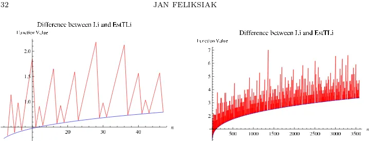
Figure 2. The drawings contrast the difference in estimation er-ror made by the Gauss’ Logarithmic Integral (black) vs the Tai-lored Integral (red). The figures drawn with respect toξ, give the range up ton= 7 919 (left), and up ton= 4 256 233 (right).
Remark 5.1. The classical offset logarithmic integralLi(n)of C.F. Gauss, is an im-provement of the estimate of the number of primes, up to somen∈Ngiven byn/logn. Therefore, since the left side of the inequality 5.1 increases only at the primes as πn does, it constitutes an improvement in π(n) estimation. Numerical comparison of the performance of the Carl F. Gauss offsetLi(n)vs theT Li(n)is given in Table 2, and graphically presented in Fig. 2.
The graph of the tailored integral is below that of π(n) for all n ∈ N | n < 43, please refer to Fig. 4a. Since the primorial function increases only at the primes, necessarily therefore, the estimation error of the tailored integral increases at the primes only. Hence, if the relation T Li(n) ≥ π(n) holds at the primes, it therefore holds at every other point. This contrasts strongly with the Gauss’ logarithmic integral Li(n) in which, the estimation error term increases over the intervals between the primes and decreases at the primes. As a result, it produces large estimation error oscillations. On the other handT Li(n), accurately duplicates the pattern of the curve ofπ(n), with minimal error increase.
Table 2. Comparison: Gauss’ Li(n) vsT Li(n)
Figure 3. The figures drawn at everyn∈Nin the range, show the graphs ofLi(n) (grey),π(n)(black) andT Li(n)(red).
Figure 4. The drawings show the estimation errorT Li(n)−π(n) curve drawn at everyn∈Nwithin the pertinent range. The right figure drawn with respect toξ, corresponding to: 3≤n≤5,000.
5.3. Tailored integral T Li(n) step sequence.
Due to the fact thatT Li(n)increases stepwise at the primes, the analysis of the step size and its limit as n approaches infinity forms the core of the proof of the tailored integral. Thus, for a pair of consecutive primes: piand pi+1 we define the stepwise limits of integration for allpi ∈N| pi≥2:
Definition 5.4 (Stepwise lower integration limit). θ1= logp(i)♯ Definition 5.5 (Stepwise upper integration limit). θ2= logp(i+1)♯ Definition 5.6 (Step sequence).
SSQ(p(i+1)) = (
T Li(p
(i+1))−T Li(pi) )
=
∫ θ2
θ1
dt
logt ∀pi∈N|pi≥3
Definition 5.7 (Step estimation error sequence).
SER(p(i+1)) = (
T Li(p
(i+1))−T Li(pi)−1 )
=
∫ θ2
θ1
dt
logt −1 ∀pi∈N|pi≥3
Remark 5.2. Both the tailored integralT Li(n)andπnare weakly monotone
which diverges to infinity. The initial estimates of the T Li(n) step size indicate that the step sequence quickly approaches the value of 1 from above. Table 3 presents some of the values that the step sequence takes at the powers of 10.
It is obvious that the numerical value attained by the step sequence at various points fluctuates as well, as a consequence of the size of the gap between the two consecutive primes (as well as the distance to the preceding prime pair). The effect however, of the gap interval length rapidly decreases aspi increases, since by
Theorem 3.6 the gaps Supremum is given byG(pi)= 5 (log10pi)
2 .
Lemma 5.8(Stepwise Convergence Of The Error of Estimation of theT Li(n)). The step sequence of the tailored logarithmic integral T Li(n) is Cauchy and converges asymptotically from above to the limit:
(5.2) lim
pi→∞ (∫ θ2
θ1
dt logt
)
= 1
Furthermore, the difference of the step integral T Li(n) and its approximation has the following bounds:
(5.3)
LDBp(i+1) =
1 5(p(i+1))
≤ [∫ θ2
θ1
dt logt −
logp(i+1) log(logp(i+1)♯
) ]
≤ 1
p(i+1)
=U DBp(i+1)
for allp∈N| p≥13
withθ1 andθ2 given by the Definitions5.4 and5.5respectively.
Proof.
By the Prime Number Theorem we may estimate the integral T Li(n) step se-quence for any prime numberp∈N|p≥3 :
(5.4)
∫ θ2
θ1
dt logt ∼
θ2−θ1 logθ2
=
(
logp(i)♯+ logp(i+1)
)
−logp(i)♯ log(logp(i+1)♯
) = logp(i+1) log(logp(i+1)♯
)
Thus by the PNT we have,
(5.5)
∫ θ2
θ1
dt logt ∼
logp(i+1) log(logp(i+1)♯
)
The logarithm of the primorial function is clearly a monotone function increasing unboundedly, hence, producing a sequence of positive real numbers which diverges to infinity. From Lemma 4.3 we have that logp(i+1)♯ is asymptotic from below to p(i+1), as well as:
logp(i+1)♯ < p(i+1)≤n ∀n∈N|n≥2,
wherep(i+1)is the greatest primep∈N| p≤n Hence, for a prime numberp∈N,
log(logp(i+1)♯
)
≤logp(i+1)
This implies that the estimating sequence converges asymptotically from above to the limit:
(5.6) lim
p(i+1)→∞ (
logp(i+1) log(logp(i+1)♯
) )
Therefore it is Cauchy. The step integralT Li(n) atp6= 13 attains∼1.13056 and the step sequence values decrease, asymptotically approaching 1 as pn increases
unboundedly. Please, also refer to the Table 3. Consequently,
(5.7) lim
p(i+1)→∞ (∫ θ2
θ1
dt logt
)
= lim
p(i+1)→∞ (
logp(i+1) log(logp(i+1)♯
) )
→1
Thus the step integralT Li(n)is Cauchy as well. BothLDBp(i+1)andU DBp(i+1)are
clearly strictly monotone decreasing Cauchy sequences. Suppose that the following assertion is false:
(5.8) 1
5(p(i+1))
≤ [∫
θ2
θ1
dt logt−
logp(i+1) log(logp(i+1)♯
) ]
This implies that:
(5.9) 5(p(i+1)) −
[
1/
(∫ θ2
θ1
dt logt −
logp(i+1) log(logp(i+1)♯
) )]
< 0
However, at p(n) = 13 the inequality 5.9 attains ∼ 48.6109 and diverges as p(n) increases unboundedly with the rate of divergence ∝k p(n) s.t. k ∼ 3 for larger primes p(n). Consequently, we have a contradiction to the hypothesis. Inequality 5.8 therefore, is valid for allpn ∈N| pn≥13.
Suppose now, that the following inequality is false:
(5.10)
[∫ θ2
θ1
dt logt−
logp(i+1) log(logp(i+1)♯
) ]
≤ 1
p(i+1)
This implies that:
(5.11)
[
1/
(∫ θ2
θ1
dt logt−
logp(i+1) log(logp(i+1)♯
) )]
− p(i+1) < 0
However, at p(n) = 13 the inequality 5.11 attains∼ 3.38914 and diverges as p(n) increases unboundedly with the rate of divergence ∝k p(n) s.t. k ∼ 1 for larger primes p(n). Consequently, we have a contradiction to the hypothesis. Inequality 5.10 therefore, is valid for allpn ∈N | pn ≥13. Necessarily this implies that the
Inequality 5.3 holds as stated. This demonstrates therefore, that sinceU DBp(i+1)
is strictly monotone decreasing Cauchy sequence with a limitL= 0:
lim (p(i+1))→∞
(
1 p(i+1)
)
= lim
(p(i+1))→∞ [∫ θ2
θ1
dt logt −
logp(i+1) log(logp(i+1)♯
) ]
→0
Thus, from above we have that the estimating sequence 5.6 converges asymptoti-cally from above to its limit L= 1. Since the step integral atp(i+1) = 11 attains
∼1.2171 necessarily therefore the step integral tends asymptotically from above:
(5.12) lim
p(i+1)→∞ (
logp(i+1) log(logp(i+1)♯
) )
= lim
p(i+1)→∞ (∫ θ2
θ1
dt logt
This implies, that the sequence of the step estimation errors asymptotically con-verges from above (also refer to Table 3):
lim
p(i+1)→∞
((∫ θ2
θ1
dt logt
) −1
)
= lim
p(i+1)→∞ (
logp(i+1) log(logp(i+1)♯
)−1
) →0
Thus concluding the proof of Lemma 5.8.
Table 3. Step sequence values
pi pi+1 Actual step Est. step Eq. 5.4 Difference 7 11 1.284296315549 1.17139190927 0.112904406279 97 101 1.036036760682 1.029877441266 0.006159319416 997 1009 1.007295189211 1.006767382731 0.000527806480 9973 10007 1.001161895309 1.001111285430 0.000050609879 99991 100003 1.000271361223 1.000266343124 5.0180995783×10⁻⁶ 999983 1000003 1.000109530674 1.00010902981 5.00863978704×10⁻⁷ 9999991 10000019 1.000029984472 1.000029934445 5.0027059524×10⁻⁸ 99999989 100000007 1.000006660234 1.000006655234 5.00067955427×10⁻⁹
Remark 5.3. The integral part of the step size clearly accounts for the prime number found. Comparing each fractional part of the step (please refer to Table 3) at pi with the corresponding term of the harmonic series (p1
i), it becomes obvious that it is greater than the term of the series. Since the error of estimation is the sum ofπ(n)of such individual terms, comparing its sum with the divergent sum of reciprocals of successive prime numbers leads to a conjecture, that the sum of the estimation error terms diverges aspi tends to infinity.
5.4. Step sequence estimation error bounds.
Corollary 5.9(Infimum and Supremum Step Sequence Estimation Error Bounds). The step sequence error of estimation of the prime counting function π(n) by the application of the tailored logarithmic integral T Li(n) ∀p(i) ∈ N | p(i) ≥ 13, is bounded below/above by:
(5.13) IN Fp(i+1) =
logp(i+1) log(logp(i+1)♯
)+ 1
5(p(i+1))− 1≤
[∫ θ2
θ1
dt logt−1
]
≤ logp(i+1) log(logp(i+1)♯
)+ 1 p(i+1)
−1 =SUPp(i+1) for allp∈N|p≥13
wherep(i)andp(i+1)are associated with lower/upper limits of integration andθ1, θ2 are given by the Definitions 5.4 and 5.5 respectively.
Proof. From Lemma 5.8 we have:
(5.14)
1 5(p(i+1))
≤ [∫ θ2
θ1
dt logt−
logp(i+1) log(logp(i+1)♯
) ]
≤ 1
p(i+1)
Which is equivalent to say that:
(5.15) logp(i+1) log(logp(i+1)♯
)+ 1
5(p(i+1))
−1≤
[∫ θ2
θ1
dt logt −1
]
≤ logp(i+1) log(logp(i+1)♯
)+ 1 p(i+1)
−1 for allp∈N|p≥13
thus completing the proof.
The Infimum and Supremum error boundsISE(p
(n)) andSSE(p(n)) for the
tai-lored integral step estimation error are computationally very demanding. Therefore, Theorems: 5.10 and 5.11 that follow, establish simpler bounds.
Theorem 5.10(The Step Sequence Estimation Error Lower Bound).
The estimation error of the tailored logarithmic integral T Li(n) at every step exceeds the value of the inverse of the pertinent prime number hence, it is bounded below by1/p∀p∈N| pi≥13:
(5.16) SER(p
(i+1)) = (∫ θ2
θ1
dt logt
)
−1> 1 p(i+1)
wherep(i)andp(i+1)are associated with the lower/upper limit of integrationθ1and θ2 respectively.
Proof.
By Lemma 5.8 the sequenceSER(p
(i+1)) is Cauchy and it converges from above
to the limit L = 0. The sequence of the reciprocals of prime numbers is clearly Cauchy and converges to the limitL= 0. By Lemma 5.8 we have that:
(5.17) 1
5(p(i+1))
+ logp(i+1) log(logp(i+1)♯
)−1≤
∫ θ2
θ1
dt
logt −1 for allp∈N|p≥13
Consequently Theorem 5.10 is valid if and only if:
(5.18) 1
p(i+1)
≤ 1
5(p(i+1))
+ logp(i+1) log(logp(i+1)♯
)−1
Now,
(5.19) 1 5(p(i+1))
+ logp(i+1) log(logp(i+1)♯
)−1− 1 p(i+1)
=
(
5(p(i+1))
(
log (p(i+1))
))
−(4 + 5(p(i+1))
) (
log(log(p(i+1)♯
))) (
5(p(i+1))
) (
log(log(p(i+1)♯
)))
From Lemma 4.3 we have that logp(i+1)♯is asymptotic (from below):
logp(i+1)♯∼p(i+1) as well as:
logp(i+1)♯ < p(i+1)≤n ∀n∈N|n≥2 Hence,
log(logp(i+1)♯
)
From Lemma 4.5 we have for allp(i+1)∈N|p(i+1)≥2: (5.20)
LBp(i+1) = (√
5−1) (4γ2−2γ) (logp(i+1)
) 3 √p
(i+1)<
(
p(i+1)−logp(i+1)♯
)
Consequently, from the above we obtain:
(5.21) (p(i+1)− LBp(i+1)>logp(i+1)♯ )
Bearing in mind that for all positivea, b∈R| a > b:
(5.22) log (a+b) = log (a(1 +b/a)) = log (a) + log
(
1 + b a
)
Thus, by Lemma 4.3 we have:
(5.23) 5p(i+1)
(
log(p(i+1)− LBp(i+1) ))
≥5p(i+1)
(
log(log(p(i+1)♯
)))
Hence,
(5.24) 5p(i+1)
(
log(p(i+1)
))
= 5p(i+1)
(
log(p(i+1)− LBp(i+1)+LBp(i+1) ))
= 5p(i+1)
[
log(p(i+1)− LBp(i+1) )
+ log
(
1 +( LBp(i+1) p(i+1)− LBp(i+1)
) )]
≥5p(i+1)
(
log(log(p(i+1)♯
)))
Suppose that the Theorem5.10is false. Then it must be true that the numer-ator of equation 5.19 is less than zero. From inequality 5.24 we see that without loss of generality, upon substitution into the numerator of the inequality 5.19, we can drop the common terms obtaining:
(5.25) (5(p(i+1))
(
log (p(i+1))
))
−(4 + 5(p(i+1))
) (
log(log(p(i+1)♯
)))
≥5p(i+1)
[
log
(
1 + ( LBp(i+1)
p(i+1)− LBp(i+1) )
)]
−4(log(log(p(i+1)♯
)))
<0
However at p(i+1) = 37 the difference 5.25 attains ∼ 0.20084385349345676 and diverges. Hence we have a contradiction to our hypothesis which implies that the inequality is true:
(5.26) 1
p(i+1)
≤ 1
5(p(i+1))
+ logp(i+1) log(logp(i+1)♯
)−1
Consequently this implies that Theorem 5.10 is satisfied for all pi ∈N | pi ≥37,
a simple computer calculation verifies that this inequality also holds within the interval 13≤pi≤37. This necessarily means that Theorem 5.10 is satisfied for all
pi∈N|pi≥13, thus completing the proof.
Theorem 5.11(The Step Sequence Estimation Error Upper Bound).
The inverse of a root of the pertinent prime number at every step exceeds the value of the estimation error of the tailored logarithmic integralT Li(n)step sequence
∀pi∈N| pi≥13:
(5.27) SER(p
(i+1)) = (∫ θ2
θ1
dt logt
)
−1< 1
a √p
(i+1)
wherep(i)andp(i+1)are associated with the lower/upper limit of integrationθ1and θ2 respectively.
Proof.
By Lemma 5.8 the sequenceSER(p
(i+1)) is Cauchy and it converges from above
to the limitL= 0. The sequence of the reciprocals of the root of prime numbers is clearly Cauchy and converges to the limitL= 0. By Lemma 5.8 we have that:
(5.28)
∫ θ2
θ1
dt
logt−1≤ 1 p(i+1)
+ logp(i+1) log(logp(i+1)♯
)−1
for allp∈N|p≥13
Consequently Theorem 5.11 is valid if and only if:
(5.29) 1
p(i+1)
+ logp(i+1) log(logp(i+1)♯
)−1≤ 1 a √p
(i+1)
wherea=π 2
Now,
(5.30) 1 (p(i+1))
+ logp(i+1) log(logp(i+1)♯
)−1− 1 a √p
(i+1) =
(
p(i+1)√ap(i+1)
(
log (p(i+1))
))
−(p(i+1)−√ap(i+1)+p(i+1)√ap(i+1)
)(
log(log(p(i+1)♯
))) (
p(i+1)√ap(i+1)
) (
log(log(p(i+1)♯
)))
From Lemma 4.3 we have that logp(i+1)♯is asymptotic (from below):
logp(i+1)♯∼p(i+1)
as well as:
logp(i+1)♯ < p(i+1)≤n ∀n∈N|n≥2
Hence,
log(logp(i+1)♯
)
≤logp(i+1)
From Lemma 4.5 we have for allp(i+1)∈N|p(i+1)≥2:
(5.31) UBp(i+1) = 2√p(i+1)>
(
p(i+1)−logp(i+1)♯
)
Consequently, from the above we obtain:
(5.32) (p(i+1)− UBp(i+1) )
<logp(i+1)♯
Bearing in mind that for all positivea, b∈R| a > b:
(5.33) log (a+b) = log (a(1 +b/a)) = log (a) + log
(
1 + b a
)
Thus, by Lemma 4.3 we have:
(5.34) p(i+1)√ap(i+1)
(
log(p(i+1)− UBp(i+1) ))
≤p(i+1)√ap(i+1)log
(
log(p(i+1)♯
Hence,
(5.35)
p(i+1)√ap(i+1)
(
log(p(i+1)
))
=p(i+1)√ap(i+1)
(
log(p(i+1)− UBp(i+1)+UBp(i+1) ))
=p(i+1)√ap(i+1)
[
log(p(i+1)− UBp(i+1) )
+ log
(
1 + ( UBp(i+1) p(i+1)− UBp(i+1)
) )]
≤p(i+1)√ap(i+1)
(
log(log(p(i+1)♯
)))
Suppose that the Theorem5.11is false. Then it must be true that the numer-ator of equation 5.30 is greater than zero. From inequality 5.35 we see that without loss of generality, upon substitution into the numerator of the inequality 5.30, we can drop the common terms obtaining:
(5.36)
(
p(i+1)√ap(i+1)
(
log (p(i+1))
))
−(p(i+1)−√ap(i+1)+p(i+1)√ap(i+1)
)(
log(log(p(i+1)♯
)))
≤p(i+1)√ap(i+1)log
(
1 + UBp(i+1) (p(i+1)− UBp(i+1))
)
−(p(i+1)−√ap(i+1)
)(
log(log(p(i+1)♯
)))
However at p(i+1) = 197 the difference 5.36 attains∼ −1.20860443 and diverges. Hence we have a contradiction to our hypothesis which implies that the inequality is true:
(5.37) 1
p(i+1)
+ logp(i+1) log(logp(i+1)♯
)−1≤ 1 a √p
(i+1)
wherea=π 2
Consequently this implies that Theorem 5.11 is satisfied for allpi ∈N| pi ≥197,
a simple computer calculation verifies that this inequality also holds within the interval 13≤pi ≤197. This necessarily means that Theorem 5.11 is satisfied for
allpi∈N|pi≥13, thus completing the proof.
Hence, by Theorems 5.10 and 5.11, for the largest prime number p(i+1) that satisfies the conditionp(i+1)≤n∈N, we have:
1 p(i+1)
<
(∫ θ2
θ1
dt logt
)
−1< 1
a √p
(i+1)
∀p(i)≥13 wherea= π 2
Remark 5.4.
We need to re-define the lower/upper limits of integration to conform with the summation limits. The computation of the sum of step errors of the integralT Lin
begins atp2= 3, irrespective of the fact that the computation of the sums pertinent to the bounds (Infimum, Supremum, Lower and Upper) begins first atp15= 47. Definition 5.12 (Theta applicable for summation). θ1= log
(
p(2+(k−1))♯
)
Definition 5.13 (Theta applicable for summation). θ2= log(p(2+k)♯