Accelerated Gradient Descent Using Instance
Eliminating Back Propagation
Farzad Hosseinali1
1 Mountain View, CA, USA 94040; [email protected]
Abstract:Artificial Intelligence is dominated by Artificial Neural Networks (ANNs). Currently, the Batch Gradient Descent (BGD) is the only solution to train ANN weights when dealing with large datasets. In this article, a modification to the BGD is proposed which significantly reduces the training time and improves the convergence. The modification, called Instance Eliminating Back Propagation (IEBP), eliminates correctly-predicted-instances from the Back Propagation. The speedup is due to the elimination ofunnecessarymatrix multiplication operations from the Back Propagation. The proposed modification does not add any training hyperparameter to the existing ones and reduces the memory consumption during the training.
Keywords:Artificial Neural Networks; Gradient Descent; Back Propagation; Instance Elimination; Speed up; Batch Size
1. Introduction
The Batch Gradient Descent (BGD) is the predominant method to minimize a loss function in an Artificial Neural Network (ANN) when dealing with large datasets. The BGD algorithm can be divided into four iterative steps: a randomized batch selection, the Forward Propagation (FP), the cost computation, and the Backward Propagation (BP).
The FP is a sequence of vectorized matrix multiplication operations, known as layers, at which a matrix of input data is multiplied by a matrix of weights. If the matrix of input data hasmnumber of instances in its rows andnnumber of features in its columns, the resulting matrix may have a different number of transformed features but always retains the same number ofmrows or instances. Within each layer, based on the ANN architecture, the resulting matrix may be fed to a non-linear activation function such as ReLU,tanh, sigmoid, softmax, etc. The output matrix of each layer is commonly referred to as its activation matrix. The objective of the FP is to come up with a prediction for the instances so that they can be matched against their corresponding, known labels (a.k.a., computing the cost).
The BP is also a sequence of vectorized matrix multiplications but in the backward direction, starting from the computed cost toward the input data. At each sequence, a computed gradient of the activation matrix for a given layer is multiplied by the transpose of the activation matrix of the previous layer (assuming layers are enumerated ascendingly in the forward direction). The resulting matrix is the gradient of the weights of the layer and is subtracted from its corresponding, randomly initiated weight matrix by a factor known as the learning rate. The BGD continues to iterate and the weights keep getting corrected until a desired level of accuracy on a validation dataset is reached (other stopping criteria also exist). For more details on BGD and ANN types, readers are referred to the online Coursera specialization on Deep Learning [1] or numerous review papers [2–4].
Recent advances in the BGD involves the implementation of the Exponentially Weighted Moving Average (EWMA) function. The modifications to the algorithm, (namely, momentum [5], RMSprop [6], ADAM [7], and NADAM [8]) use an EWMA of gradients to update the weight matrices. The purpose of using the EWMA function is to damp out large oscillations in certain dimensions as a gradient of weights is moving toward a global minimum; therefore, larger learning rates can be used and weights converge to a global minimum faster.
In this study, another approach is taken to further accelerate the BGD convergence. Hypothetically speaking, during each training iteration, the FP makes a certain prediction for instances in a batch. The author hypothesizes that the BGD may run faster if correctly-predicted-instances are eliminated during the BP. This notion stems from a common trial and error problem-solving scheme in which an intelligent system is only penalized once a mistake is made during the learning process. In the rest of this article, the hypothesis is being tested using a modified version of the BP algorithm, called Instance Eliminating Back Propagation (IEBP).
2. Algorithms
2.1. Standard BGD with ADAM
A typical BGD optimizer with the ADAM method is implemented to minimize a loss function for an ANN. The ANN has an input, an output, and a hidden layer; the dimension of the layers will be defined in the experimental section. To reduce the bulk of mathematical expressions, the bias term is not included in the ANN model. The following notations are used throughout this paper:
• Superscript[l]identifies a quantity associated with thelthlayer.
• Superscript(i)identifies a quantity associated with theithexample.
• Lowerscript(j)identifies thejthentry of a vector.
As explained earlier, within each layer of the FP, the activation matrix of the previous layerA[l−1] is multiplied by the weight matrix of the current layerW[l]. To incorporate nonlinearity into the model, the resulting matrixZ[l]is fed into thetanhactivation function.
(
Z[l] =A[l−1]W[l]
A[l] =tanh(Z[l]) (1)
In the case of layer 1,A[1−1] =A[0] =X, whereXis the input matrix of data. Throughout this paper, for any activation matrix, the rows representminstances (or examples) and the columns represent n[l]features (or transformed features). The activation function of the final layer isso f tmaxfunction. Simply put,so f tmaxcomputes the class probability for a given instance. The activation matrix of the final layer, which its shape is the same as the one-hot representation of the label matrixYoh, is called ˆY.
At the core of the BGD is a loss functionLwhich needs to be minimized. Equation 2 is the loss function used in this study. As defined earlier,y((ij))denotes the binary value (either 0 or 1) ofjthclass of instancei; likewise, ˆy((ij))denotes the computed probability forjthclass of instancei.
L(yˆ(i),y(i)) =−1
m
m
∑
i=1
N
∑
j=1
(y((ij))logyˆ((ij))+ (1−y((ij)))log1−yˆ((ij))) (2)
The objective of the BP is to compute ∂L
∂W[l] for each layer. For the special case of the final output layer, ∂L
∂W[last] is computed as follows: ∂L
∂A[last] =dA
[last]= −Y
ˆ
Y +
1−Y
1−Yˆ
∂L
∂Z[last] = ∂ L ∂A[last]∂
A[last]
∂Z[last] =dZ[last]=Yˆ−Yoh ∂L
∂W[last] = ∂ L ∂A[last]∂
A[last] ∂Z[last] ∂
Z[last] ∂W[last] =dW
[last] = 1
mA[last−1]TdZ[last]
∂L
∂A[last−1] =dA
[last−1]=dZ[last]W[last]T
(3)
In practice,dA[last]computation is not implemented sincedZ[last]derivation already includesdA[last] as a part of the chain rule. Therefore, the BP algorithm starts fromdZ[last] =Yˆ−Yohand continues
The computation ofdW[last]for other layers (in the direction starting from the output layer toward the input layer) is as follows.
dZ[l]=dA[l]∗g0(Z[l]) dW[l] = 1
mA[l−1]TdZ[l]
dA[l−1] =dZ[l]W[l]T
(4)
Here, g0(Z[l]) coresponds to ∂g
∂Z[l] which is the slope of the activation function at Z
[l]. Sincetanh activation function is used for the input and the hidden layers, thereforeg[l]0(z) =1−A[l]2.
AsdW[l]is being computed for a given layer, its EWMA is used to update the correspondingW[l] by a method called ADAM. The method includes the following steps:
vdW[l] =β1vdW[l]+ (1−β1)dW[l]
sdW[l]=β2sdW[l]+ (1−β2)dW[l]2
W[l]=W[l]−α
v
dW[l]
√
s
dW[l]+ε
(5)
Here,β1andβ2are the training hyperparameters between 0 and 1 that control the EWMA matrices
vdW[l]andsdW[l]. The hyperparameter 0<α<1 is the learning rate. To avoid division by 0, the very small constant value ofεis added to the denominator. All the matrices in Equation 5 have the same shape and all the operations are elementwise.
Some implementation of the ADAM also include the bias correction terms forvdW[l] andsdW[l]. The bias correction terms are only implemented to improve average estimations of the weights for the first few BGD iterations. After 10 or more BGD iterations,vdW[l]andsdW[l]have already stored enough number of observations to provide accurate estimation of the EWMAs. In this study, the bias correction terms are not included in the BP since a large number of iterations will be conducted before performance measures are applied. (Technically speaking, enough iterations will be provided to warm up the averages!)
A single iteration of the BGD includes an FP and its corresponding BP. For the next iteration, another batch of untrained instances is randomly selected and the FP/BP runs again. Once all the batches are finished (i.e., all the instances of the training dataset are fitted), it is commonly said that an epoch is completed. By the end of an epoch, the training dataset instances are shuffled, a new randomized batch of data is selected, and the BGD iterations continue. The termination criteria can be the total training time, certain prediction accuracy on the validation dataset, or a particular number of iterations/epochs. (A validation dataset is that portion of the original dataset on which the ANN model is not trained.)
The weights matricesW[l]and their correspondingv
dW[l]andsdW[l]are only initialized once at the beginning of the algorithm. Matrix initilization implies the creation of a matrix with a known shape but uncertain values. As the BGD iterations continue over epochs, the matrices values only get updated (using the computeddW[l]). The weights matricesW[l]are initialized using Xavier method. (That is, the normally distributed weights with average 0 and standard deviation 1 are multiplied by
q 2
n[l−1]−n[l].)vdW[l]andsdW[l]are initialized with zero values. 2.2. BGD with IEBP and ADAM
In the BGD with an IEBP, the FP is conducted in its standard form. However, the BP is only performed on the incorrectly-predicted-instances. That is, ˆYis fed to anargmaxfunction which returns the indexjof the maximum class probability for a given instance. The resultingm×1 column vector
ˆ
YFPis matched against the labelY. Indices of the wrong predictions are identified and stored in the
( ˆ
YFP=argmax(Yˆ)
mBP ={x∈Rm×1|yˆ(FPx)6=y(x)}
(6)
Instances withmBPindices are separated fromA[l]and ˆYand stored in the correspondingA[BPl]
and ˆYBP. TheW[l]correction continues similar to the standard BP.
( ˆ
YBP ={yˆ(x)|x∈mBP}
A[BPl] ={a[l](x)|x ∈mBP}
(7)
The BGD algorithm with IEBP and ADAM can be summarized as follows.
Require: Loss functionL
Require: shuffledXtrainandYtrain
Require: α,β1, andβ2such that{x∈R1|0<x <1}
Require: W[l] ← {x∈Rn[l]×n[l+1]
|x∼ N(0, 1)} Require: vdW[l]andsdW[l]such that{x∈Rn
[l]×n[l+1]
|x=0} while Wis not converged do
X,Y←minstances fromXtrain,Ytrain
mBP ← {x∈Rm×1|yˆ(FPx)6=y(x)}
A[BPl] ← {a[l](x)|x∈mBP}
dW[l]← 1
mBPA [l−1]T BP dZ
[l]
BP
updateW[l]using the ADAM method end while
return W
2.3. BGD with Random IEBP and ADAM
To validate that the potential increased efficiency in the IEBP is not due to chance, another version of the IEBP is implemented in which instances are eliminated randomly in the BP. We call this algorithm the Random IEBP. The algorithm is similar to the IEBP except that, after counting the correctly-predicted-instances from the FP, the equivalent number of randomly-selected-instances is removed from the BP. The removed instances can be either correctly- or incorrectly-predicted instances. The Random IEBP allows us to conclude whether the potential improvement in the BGD is indeed due to the elimination of the correctly-predicted-instances from the BP.
3. Experiments
3.1. Dataset
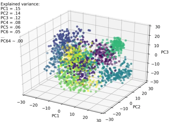
The labeled dataset used for this article is the famous hand-written digits dataset [9]. It is commonly used by machine learning practitioners to benchmark classifiers’ performance. It includes 5620 instances of 8×8, gray-scale images (i.e., 64 features for a flattened image) of hand-written digits (i.e., 10 target classes). Figure 1 shows a few instances from the dataset. Figure 2 shows a 3D scatterplot of the dataset in the Principal Component (PC) hyperspace. (The PC transformation is merely for a demonstration purpose. The transformed features were not fed into the ANN model.)
Figure 2.PC plot showing the multivariate variation among 5620 images of the hand-written digits; label colors correspond to 10 target classes. The first three PCs account for 41% of the total variance.
3.2. Model fitting
The shuffled dataset was split to training and validation datasets in a stratified manner with 9 : 1 ratio. The ANN model was fitted to the training dataset using the BGD algorithms described earlier. The training hyperparameters were set to the following values: n[l] ={30, 20, 10},α =.7, β1 = .9,
β2 = .99, ande = 10−8. For flattened images, the input feature dimensionn[0] = 8×8= 64. The algorithms were tested on different batch sizesmb = {32, 64, 128, 256}. To obtain the variability of
performance measures, the algorithms were replicated on each batch sizemb[j]for 50 times. Three performance measures were recorded for each replication: (i) the training time per epoch, (ii) the prediction accuracy on the validation dataset per epoch, and (iii) the cost per epoch.
Two criteria are used to compare algorithms functionality: (i) the maximum accuracy convergence and (ii) the percentage of relative change in the training time. in this article, the maximum accuracy convergence is the algorithm’s ability to reach its maximum accuracy on the validation dataset throughout the training process. The percentage of relative change in the training timedtbetween two
algorithms is computed using
dt= t2
−t1
t2
×100 (8)
where,tis the training time. 4. Results and Discussion
Figure 3 shows the cost and the accuracy of the validation dataset throughout training for the batch sizes 16. The plot of all three algorithms corresponds to their performance as they ran on an equal number of epochs. Form=16, the algorithms were run on 940 epochs. As can be noted, with the decrease in the cost value, the accuracy of the validation dataset increases. This indicates that the weights are being learned. As far as the training time is concerned, the IEBP has outperformed two other algorithms. Compared to the standard BGD, there has been an average 95% reduction in the training time when the IEBP is implemented. This corresponds to∼20 times training speed up. Such a high value ofdtis due to the elimination ofunnecessarymatrix multiplication operations from the BP.
Figure 3.The learning curve and the accuracy on the validation dataset as measured at the end of epochs form=16; In all figures, the error bars indicate the standard deviation of the measured random variables.
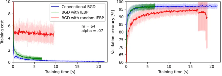
Figure 4 shows the cost and the accuracy of the validation dataset for batch sizes 64. Similar conclusions tom=16 can be made here. It took 7s for the BGD with IEBP to finish 600 epochs while the standard BGD finished the same number of epochs in 21s. This corresponds todt=74% and∼3.8
times speed up. Concerning the accuracy of the validation dataset, both the BGD and the BGD with IEBP converged to the same value of 97% almost at the same time. The Random IEBP did not perform as well as the IEBP and started to fail at the end of the training.
Figure 4.The learning curve and the accuracy as measured at the end of epochs form=64
The cost and the accuracy curves for batch size 512 and 1024 are shown in Figures 5 and 6 respectively. The BGD with IEBP outperformed two other algorithms in terms of the training speed in both batch sizes (1030 epochs were completed form = 512 and 515 epochs were completed for m=1024). For the 512 batch size,dt=31% and, for the 1024 batch size,dt=41%. In these two larger
Figure 5.The learning curve and the accuracy as measured at the end of epochs form=512
Figure 6.The learning curve and the accuracy as measured at the end of epochs form=1024
The variation indtfor different batch sizes can be summarized in Figure 7. All training was
performed on 200 epochs. Under the task of 200 epochs,dtis much higher for smaller batch sizes. For
the smaller batch size, the weights are more frequently updated; therefore, more correct predictions are made by the FP. As a result, after certain iterations, the BP is conducted on fewer instances or no instances at all. In general, the IEBP is effective as long as the computation cost of the finding incorrectly-predicted-instances is less than that of the matrix operation of eliminated instances. This is a very likely case for almost all ANNs (especially the large ones) and once the weights start to learn to make a few correct predictions.
5. Conclusions
A modification to the standard BP is introduced. The proposed algorithm, called IEBP, reduced the training time for all tested batch sizes and improved the convergence for the larger batch sizes. The IEBP removes correctly-predicted-instances from the BP. The speedup is due to the removal ofunnecessarymatrix multiplication operations from the BP. Since the algorithm with the random elimination of the instances did not converge successfully, it was concluded that the improvement in the IEBP is not due to chance. The IEBP offers the following advantages: (i) it does not add any new training hyperparameter to the existing ones; (ii) a new stopping criterion can be included based on the remaining number of instances in iterations; (iii) it reduces the memory consumption during the training; and (iv) it can be easily implemented into existing deep learning platforms. In the future works, the IEBP can be combined with regularizer algorithms and implemented in other variants of neural networks such as Convoluted and Recurrent Neural Networks.
Funding:This research received no external funding.
Conflicts of Interest:The author declares no conflict of interest.
Abbreviations
The following abbreviations are used in this manuscript:
ANN Artificial Neural Network BGD Batch Gradient Descent
BP Backward Propagation
EWMA Exponentially Weighted Moving Average
FP Forward Propagation
IEBP Instance Eliminating Back Propagation
PC Principal Component
References
1. https://www.deeplearning.ai/
2. LeCun, Y.; Bengio, Y.; Hinton, G. Deep learning.Nature2015,521(7553), 436-444.
3. Bottou, L. Stochastic gradient descent tricks.Neural networks: Tricks of the trade2012, 421–436.
4. Ruder, S. An overview of gradient descent optimization algorithms.arXiv preprint arXiv:1609.047472016. 5. Qian, N. On the momentum term in gradient descent learning algorithms.Neural networks1999,12, 145–151. 6. Hinton, G. Lecture note 6a: overview of mini-batch gradient descent.Neural Networks for Machine Learning,
University of Toronto on Coursera2012.
7. Kingma, D; Ba, J. Adam: A method for stochastic optimization.arXiv preprint arXiv:1412.69802014. 8. Dozat, T. Incorporating nesterov momentum into adam.Workshop track - ICLR,2016, 1–4.