Article
1
Bayesian Approach for Estimating the Probability of
2
Cartel Penalization under the Leniency Program
3
Jihyun Park 1, Juhyun Lee 2 and Suneung Ahn 3,*
4
1 Department of Industrial and Management Engineering, Hanyang University, Seoul, 04763, South Korea;
5
6
2 Department of Industrial and Management Engineering, Hanyang University, Seoul, 04763, South Korea;
7
8
3 Department of Industrial and Management Engineering, Hanyang University ERICA, Ansan, 15588, Korea;
9
10
* Correspondence: [email protected]; Tel.: +82-031-400-5267
11
12
Abstract: Cartels cause tremendous damage to the market economy and disadvantage consumers by causing
13
higher prices and lower quality; moreover, they are difficult to detect. We need to prevent them by scientific
14
analysis, which includes the determination of an indicator to explain antitrust enforcement. Particularly, the
15
probability of cartel penalization is a useful indicator for the evaluation of the competition enforcement. This
16
study is to estimate the probability of cartel penalization by using a Bayesian approach. In the empirical study,
17
the probability of cartel penalization is estimated by Bayesian approach from cartel data of Department of
18
Justice in United States from 1970 to 2009. The probability of cartel penalization is seen to be sensitive to
19
change of competition law and the results shows the usefulness of higher interpretation than other research.
20
The result of the policy simulation shows how effective the leniency program is. From this estimation,
21
antitrust enforcement is evaluated, and thereby, can be improved.
22
Keywords: Bayesian approach; Conjugate prior; Cartel; Leniency program; Policy simulation
23
1. Introduction
24
Cartels cause tremendous damage to perfect competition market and consumers by effectually
25
applying upward pressure on prices and downward pressure on quality; moreover, cartel has
26
difficulty in detecting because of its tacit nature. In this way of course, cartels mitigate against
27
perfect competition under which consumers are offered the best goods and services at the lowest
28
possible prices. Antitrust authorities have sought continuously to maintain the free-market system
29
against cartels, but with only partial and limited success.
30
In the previous research, the probability of cartel detection was the key indicator for measuring
31
the effectiveness of antitrust policy. The more the probability of cartel detection increases, the more
32
the expected penalties will increase, and therefore, the lesser the likelihood of cartel formation. On
33
this principle, it is possible to measure the deterrence effect according to the change of antitrust
34
policy. Markov transition process and the birth and death process were widely used. Bryant and
35
Eckard [1] constructed the birth and death process model to empirically analyze cartel data
36
provided by the US Department of Justice, estimating that the probability of cartel detection in the
37
US (United States) between 1961 and 1988 was 13-17%. By using the same method, Combe et al. [2]
38
estimated EC (European Commission) cartel detection probabilities of 12.9-13.2% for the years 1969
39
to 2007.
40
When the birth and death model has two states of competitive and collusive, the lifetimes and
41
inter-arrival times between the births of cartels are independent and exponential distributions with
42
means 1
and 1
. The number of cartels at a particular time follows a Poisson distribution
43
with mean 2
( / ){1 T}
T e
. Both Bryant and Eckard [1] and Combe et al. [2] assumed that the
44
every cartel will be eventually caught and prosecuted. But this assumption is not realistic, because
45
some cases are not penalized despite having been detected.
46
Further, Bryant and Eckard [1] and Combe et al. [2] failed to take account of the unobservable
47
cartel population. For estimation of the unobservable population, J. E. Harrington and Chang [3]
48
developed the birth and death model from that noted above. They concluded that cartel duration
49
can be a good indicator of whether a new competition law has a significant cartel-dissolution effect.
50
Using Harrington and Chang [3]’s model, Zhou [4] analyzed EC (European Commission) cartel
51
data from 1985 to 2012, concluding that the EU’s new leniency program in 2002 had had an effect in
52
deterring cartels.
53
In the research of Bryant and Eckard [1] and Combe et al. [2], Harrington and Chang [3], and
54
Zhou[4], the probability of cartel detection, as derived from cartel duration, entails the
55
determination of the time-average probability from continuous variables. On the other hand, there
56
is research indicating that the probability of cartel detection represents the ensemble-average
57
probability obtained from discrete variables such as caseloads. The time-average probability is
58
defined as the proportion of time in occupying a particular state among the total time, and the
59
ensemble-average probability is defined as the likelihood of the number of particular state among
60
the number of entire state in picking randomly at the particular time in stochastic process theory [5,
61
6].
62
Miller [7] formulated a cartel behavior model using the Markov process and used the number
63
of cartel cases as discrete variables. The model assumed that the cartel transition process is in a
64
non-absorbing and first-order Markov chain in contrast with the previous Markov models, and
65
showed the change of the number of cartel detections before and after a leniency program. He
66
concluded that the introduction of this leniency program in 1993 had increased the detection and
67
deterrence capabilities of competition enforcement. The previous research above-noted [1-4, 7] used
68
the Markov process models. This research had two notable points.
69
First, the duration of cartels and inter-arrival times between cartels follow exponential
70
distributions. To verify this assumption, it needs to be carrying out hypothesis testing of the null
71
hypothesis ‘the distribution is exponentially’. The cumulative distribution function F xˆ
of72
durations and inter-arrival time is given by
73
74
ˆ
number of observations x F x
total number of observations
.
75
76
Under the exponential distribution, log 1
F xˆ
should be approximately linear in . These77
previous works result that cartels duration and inter-arrival times between cartels follow the
78
exponential distribution; therefore, models can apply to the Markov process [7].
79
Second, this research assumed that the cartel process have to be stationary, for adopting
80
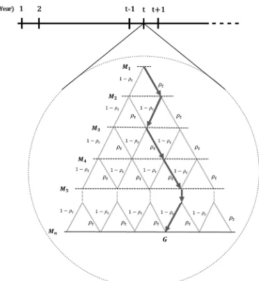
Markov process, and that when the cartel process attains the steady-state, the values can be
81
analyzed. This is also unrealistic. In the research of Bryant and Eckard [1] and Combe et al. [2], the
82
probability is the result value when it reaches in the steady-state. This kind of probability is called
83
time-independent probability. Otherwise, estimation needs to be proceeded by a form of
84
time-dependency rather than time-independency, because the purpose of estimating the probability
85
of cartel detection is evaluating the effects of varying competition policies [8]. Thus, Hinloopen [8]’s
86
research was theoretical literature for analyzing a subgame of collusion.
87
A new mathematical methodology in the form of a non-Markov process recently has been
88
emerged. Ormosi [9] estimated the annual probability of cartel detection by employing methods of
89
capture-recapture based on EC information in the period between 1981 and 2001. These methods of
90
Ormosi [9], frequently used in ecology, reflect the fact that transition parameters are not
91
steady-state, and further, that detection and survival rates are time-independent. However, there
92
are two unreasonable assumptions. First, capture-recapture methods assume that the number of
93
temporary migrations between the two states (compete-collude) do not exist; thus, they are
94
regarded as robust design methods. The antitrust policy tends to be largely varied by governmental
95
specifically in the moving average of three or five years. If the probability is used on the basis of one
97
year, the accuracy of probability can be decreased, due to data insufficiency. The market reacts
98
immediately to competition law changes; therefore, the probability needs to be estimated for the
99
smallest unit of time.
100
This paper is to estimate the probability of cartel penalization by using Bayesian approach and
101
evaluate the impact of leniency program as antitrust policy. This study uses the conjugate family of
102
Beta-binomial in that cartel occurs in binomial events. The posterior mean of beta-binomial
103
distribution means the probability of cartel penalization in year. It shows the trend of the
104
probability of cartel penalization, and then it can improve the antitrust policy from the measured
105
impact of leniency program. In this light, the present research makes three contributions.
106
Firstly, this paper estimate the probability of cartel penalization for analyzing the cartel, in
107
contrast to the probability of cartel detection treated in previous research. The probability of cartel
108
detection which means that unobserved cartel must be caught to antitrust authority is a useful
109
decision making for company. However, the probability of cartel penalization means penalization
110
odds of detected cartel through sufficient investigation. It is used as an indicator of evaluating the
111
impact of leniency program and the capability of antitrust authority.
112
Secondly, the methodology of this paper makes up for the weak points of previous methods of
113
probability estimation. The previous methods have lots of unrealistic assumptions; such as the
114
analyzed case is the eventually caught/detected case and the time-average probability etc. To
115
improve the assumptions, we need to estimate the time dependent ensemble-average probability
116
based on the caseloads that is more practical than time-average probability for sensitive estimation
117
of probability.
118
Thirdly, this study shows that the Bayesian approach could play a practical role in modeling
119
and analysis of the cartel situation. The Markov process model which is commonly used in
120
previous research is essential consideration ‘in the steady-state probability’; however, it is difficult
121
to assume ‘in the steady-state probability’ because cartel case is continuously varied over time. The
122
probability of cartel penalization is estimated by using subjective approach of Bayesian theory. The
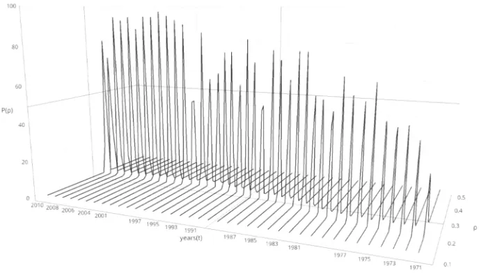
123
subjective approach to probability estimation can contain a lot of uncertainty, but it has a good
124
predictive performance in itself [10]. The bias caused by the subjective approach could be solved
125
from the Bayesian update procedure. In addition, we present reliable result by using
126
non-informative prior and conjugate prior distribution when prior information is not sufficient.
127
The paper is organized as follows. Section 2 defines the penalization probability and Bayesian
128
probabilistic model. Section 3 presents an empirical study based on US cartel data. Section 4 draws
129
conclusions.
130
2. Bayesian probabilistic model
131
When faced with suspected cartel cases, a competition authority carries out an initial
132
investigation to determine if there are sufficient grounds to prosecute. Prosecuted cartels will be
133
penalized in the form of fines through the trial. Eventually, the three states of cartel cases are
134
commonly detection, prosecution, and penalization [11]. The estimated probability of this study is
135
based on the detection and penalization states. The probability of cartel penalization ( ) is described
136
as the proportion of the number of penalizing cases to detecting cases in year t (t1, 2, ).
137
Estimation of penalization probability by using Bayesian approach involves two assumptions.
138
First, unit of case is market. Accordingly, the research of Bryant and Eckard [1] and Miller [7] is
139
based on the unit of the market. Bos and Harrington [12] argued that firm-based analysis is more
140
realistic; nonetheless, for ease of analysis, the present study was based on the unit of the market. In
141
practice, the cartels participate in all firms of the market. Second, a cartel arises only as one event
142
during one year. Every cartel is transferred to the competition as the result of punishment by the
143
authorities. This is called the ‘Grim trigger strategy’ [13, 14]. If some player deviates from the cartel,
144
thereafter, the game cannot be colluded indefinitely.
145
This study constructed a Bayesian probabilistic model to estimate the probability of cartel
146
posterior distribution. In order to infer a posterior distribution, it is necessary to determine the
148
proper prior distribution. A Bayesian probabilistic model is comprised of a prior distribution to
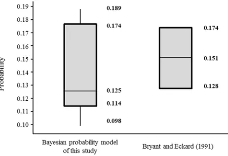
149
induce a posterior distribution, hyperparameters, and a likelihood function. By means of Bayesian
150
sequential analysis of dynamic Bayesian model, it can reflect the latest trends of time series data [15,
151
16].
152
To induce a posterior distribution from a prior distribution, two things should be considered:
153
the likelihood function, and the parameters in the prior distribution, which are known as
154
hyperparameters [17]. In the Bayesian approach, the natural conjugate prior distribution generally
155
has been recommended, because its functional form is similar to the likelihood distribution [18, 19].
156
Therefore, in order to adopt the notion of natural conjugacy, we have to determine the appropriate
157
likelihood function. Consider the following notations for Bayesian probabilistic model.
158
159
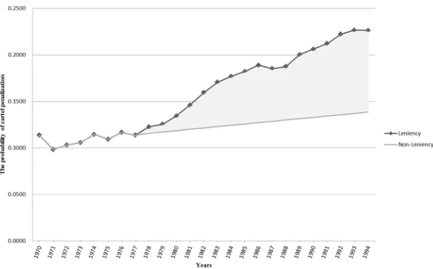
: The probability of cartel penalization cases in year t
160
: The number of cartel detection cases by the competition authority at the end of year t
161
: The number of cartel penalization cases by the competition authority at the end of year t
162
163
When the detected market participating in cartel is n, Fig. 1 shows the process of cartel
164
formulation and demise in year t.
165
166
167
Figure 1. Estimating the probability of cartel penalization through path problem
168
169
In the Fig. 1, M M1, 2,,Mn is detecting the market of cartel in year t. Arrows in path show
170
whether the detected cartels will be finally penalized. When the direction of arrow is right side, this
171
cartel will be finally penalized; otherwise, not penalized. For example, the market M2 is left side
172
direction; this means the market M2 will be not finally penalized as the probability . This study
173
wants to infer probability of market n+1 penalization in the path G. This probability is estimating
174
likelihood function based on the data from market 1 to n and the prior distribution, besides,
175
inferring a posterior distribution from Bayesian approach [13]. The expectation of posterior
176
distribution means the probability of cartel penalization.
177
2.1. Likelihood function and prior distribution
178
The number of cases is investigated at the end of year t, and each case follows the Bernoulli
179
process with an independent and identical distribution. Therefore, the Bernoulli random variable
180
i
X with one case shown is given by
181
i
1 if penalizing with probability X
0 if non - penalizing with probability 1 ,
183
where i is the number of cartel firm in the market (i 1, ,nt) and 01. The probability mass
184
function of the random variable, known as the Bernoulli probability, is given by
185
186
1 ( ) xi(1 ) xi.
i
f x
(1)
187
Once the number of cases is investigated and is penalized at the end of year t, the joint
188
probability mass function of cartel cases is given by
189
190
1 1 1 1 ( , , ) ( ) (1 ) (1 )(1 ) . t
t
t
i i
i t i
t t t
n n i i n x x i
x n x
k n k
f x x f x
(2)191
The probability of cartel penalization has a value between 0 and 1. In Equation (2), P
is a192
binomial form as likelihood function, because there are only two final states of a cartel: whether
193
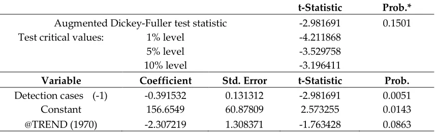
penalization or not. Thus, we use the beta distribution as a prior distribution based on the natural
194
conjugacy [17, 20]. The prior distribution P
is the beta distribution with hyperparameters α195
and β; thus, the probability density function is given by
196
197
1
1 1 ,
P
(3)
where ( 0) and ( 0) are the hyperparameters. The function ( ) is a gamma function, which
198
is defined as
199
200
1 0
( ) e xx dx.
(4)Note that when α is a positive integer, ( ) (1)!.
201
2.2. Bayesian estimation
202
In the Bayesian approach, the posterior distribution is given by
203
204
1 1 1 , , , , , . , , t t t n n nP x x
P x x
P x x
(5)
205
The joint probability distribution P x
1,,xnt,
in Equation (5), which reflects the206
multiplicative laws of probability in Equations (2) and (3), is
207
208
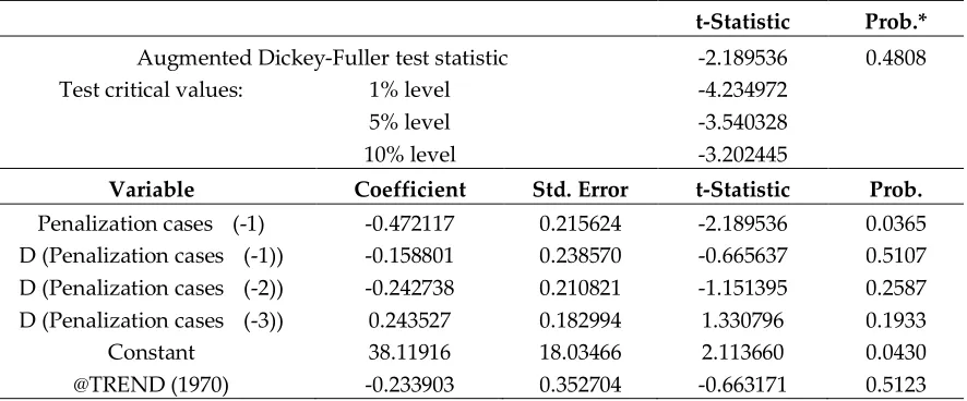
1 1 1 1 , , , , , 1 . t t t t t n n n k kP x x P x x P
The marginal probability distribution P x
1, ,xnt
, calculated by the law of total probability, is210
given by211
212
1 1 1 01 1 1
0
1 1 1
0 , , , , , 1 1 . t t t t t t t t n n n k k n k k
P x x P x x d
d d
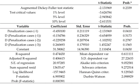
(7)Note that
1 1 1
0 1
t t
t n k t t t
k
t
k n k
d n
.213
Suppose that the initial probability ( ) is 0.5 meaning whether the detected or the non-detected
214
case for eliminating the dependence on the prior information. Thus, the hyperparameters α and β
215
of the prior distribution are 1 as a noninformative prior. Therefore, the posterior distribution is a
216
beta distribution with the parameters kt and nt kt. The posterior distribution of Equation
217
(5) is represented by
218
219
1 1 1 1 1 1 , , ( ) 1 . ( ) ( ) t t t t t t t n k k nt t t
t
n k
k t
t t t
P x x
k n k
n n
k n k
(8)
220
The posterior mean E x1, , xnt from Equation (8) is
221
222
11 0 1
1 1 1
0
1 ( 1) 1 ( ) 1
0 , , , , ( ) 1 ( ) ( ) ( ) 1 ( ) ( ) 1 ( ) ( ) ( ) t t t t t t t t n n n k k t
t t t
n k
k t
t t t
t t t
t
t t t t
E x x P x x d
n
d
k n k
n
d
k n k
k n k
n
k n k n
1
. t t k n (9)
3. Empirical study
223
3.1. Data
224
This study uses data from Workload statistics published by the Antitrust Division of the
225
Department of Justice (DOJ) for the period between 1970 and 2009 [21]. It contains the annual
226
statistics of penalized cases and detected cases by criminal enforcement and civil enforcement of
227
district courts, with respect to the laws of Sherman §1-Restraint of Trade, Sherman §2-Monopoly,
228
and Clayton §7-Mergers. The antitrust division prosecutes in the form of criminal enforcement
229
cases if the cartels, known as “hard-core cartels,” are determined by preliminary examination to
230
enforcement cases. This study does not consider the appellate cases and the cases of contemporary
232
criminal-civil enforcement at the same time, due to a little case.
233
3.2. Time series analysis
234
Prior to the model application, a time series analysis was implemented for the purposes of
235
testing stability, or in other words, to eliminate spurious relations wrongly inferred to be related.
236
The study, alternatively, employed the augmented Dickey-Fuller (ADF) unit root test to confirm the
237
stability of time series data (details are provided in Appendix A).
238
If the result shows that time series data is unstable, the difference-stationary process is needed.
239
The representative method for stabilizing time series data is order difference or log order difference.
240
However, using order difference, it is possible that the meaning of original data will be lost, leading
241
to different conclusions in the economy [22]. Economic variables such as price, currency and stock
242
index cannot be used to verify the stability of time series data, because they are commonly
243
non-stationary data [23].
244
3.3. Results
245
The empirical study, using the model defined in Section 2, drew an annual beta distribution for
246
the probability of cartel penalization. The results are summarized in Table 1 and Fig. 2 illustrates
247
the distribution every years.
248
Table1. The probability of cartel penalization through Bayesian sequential analysis
249
Years (t) Detection cases (n) Penalization cases (k) Prior α Prior β Posterior α Posterior β The expected probability of cartel penalization ( )
1970 (1) 473 53 1 1 54 421
1971 (2) 593 51 54 421 105 963 0.11368
1972 (3) 465 53 105 963 158 1375 0.09831
1973 (4) 538 61 158 1375 219 1852 0.10307
1974 (5) 338 57 219 1852 276 2133 0.10575
1975 (6) 381 29 276 2133 305 2485 0.11457
1976 (7) 374 64 305 2485 369 2795 0.10932
1977 (8) 484 46 369 2795 415 3233 0.11662
1978 (9) 290 68 415 3233 483 3455 0.11376
1979 (10) 407 62 483 3455 545 3800 0.12265
1980 (11) 377 89 545 3800 634 4088 0.12543
1981 (12) 255 93 634 4088 727 4250 0.13427
1982 (13) 262 109 727 4250 836 4403 0.14607
1983 (14) 245 99 836 4403 935 4549 0.15957
1984 (15) 257 80 935 4549 1015 4726 0.17050
1985 (16) 254 77 1015 4726 1092 4903 0.17680
1986 (17) 307 98 1092 4903 1190 5112 0.18215
1987 (18) 270 27 1190 5112 1217 5355 0.18883
1988 (19) 216 55 1217 5355 1272 5516 0.18518
1989 (20) 220 132 1272 5516 1404 5604 0.18739
1990 (21) 178 77 1404 5604 1481 5705 0.20034
1991 (22) 178 81 1481 5705 1562 5802 0.20610
1992 (23) 176 113 1562 5802 1675 5865 0.21211
1993 (24) 224 84 1675 5865 1759 6005 0.22215
1994 (25) 269 58 1759 6005 1817 6216 0.22656
1995 (26) 249 86 1817 6216 1903 6379 0.22619
1996 (27) 436 59 1903 6379 1962 6756 0.22978
1997 (28) 454 64 1962 6756 2026 7146 0.22505
1998 (29) 408 89 2026 7146 2115 7465 0.22089
1999 (30) 373 69 2115 7465 2184 7769 0.22077
2000 (31) 261 64 2184 7769 2248 7966 0.21943
2001 (32) 225 61 2248 7966 2309 8130 0.22009
2002 (33) 192 50 2309 8130 2359 8272 0.22119
2003 (34) 218 43 2359 8272 2402 8447 0.22190
2004 (35) 171 46 2402 8447 2448 8572 0.22140
2005 (36) 217 42 2448 8572 2490 8747 0.22214
2006 (37) 204 48 2490 8747 2538 8903 0.22159
2007 (38) 186 40 2538 8903 2578 9049 0.22183
2008 (39) 172 58 2578 9049 2636 9163 0.22173
2009 (40) 164 83 2636 9163 2719 9244 0.22341
2010 (41) 0.22728
251
Figure 2. Annual beta distributions about the probability of cartel penalization
252
253
Fig. 2 shows that the probability distribution is increasing trend in the right-hand direction
254
with time. Bayesian inference theory specifies that a beta distribution, with updating, will tend to
255
converge on one point [17]. Indeed, the result shows convergence of the present distribution on the
256
one point at around 0.22. Next, we were able to calculate the posterior mean by Equation (9). In the
257
Fig. 3, accordingly, illustrates the annual expected probability of cartel penalization.
258
259
260
Figure 3. The annual probability of cartel penalization
261
262
In the late 19th century, the United States was confronted with a very significant change:
263
large-scale manufacturing interests emerged, in great numbers, and enjoyed excessive economic
264
power. In response, the Interstate Commerce Act in 1887 began a shift towards federal rather than
265
state regulation of big business. This was followed by the Sherman Antitrust Act in 1890, which is
266
the basis of US competition laws. Later, the Clayton Antitrust Act in 1914, enacted to prohibit price
267
discrimination, corporate mergers and interlocking directorates.
268
We can now show how the change of probability of cartel penalization is impacted on the
269
antitrust laws in the analysis periods. The Antitrust Penalty and Procedure Act in 1974, known as
270
the Tunney Act, required that prospective mergers and acquisitions obtain approval from the DOJ.
271
In 1976, the Hart-Scott-Rodino Antitrust Improvements Act was passed, and in 1978, the Leniency
272
program was instituted. At this notable time, the probability of cartel penalization was increasing.
273
At the peak of cartel penalization probability, in 1994, DOJ reformed the Leniency program. The
274
investigations. Fig. 3 indicates that since 1994, the probability has been steady and stable. Clearly,
276
the reform of competition laws, as well as the enacting of additional such laws, had an impact on
277
the market. Commonly in fact, the market adjusts to changes of antitrust policy.
278
3.4. Model Comparison
279
Chang and Harrington [24] constructed a Markov process model to consider the stochastic
280
formation and demise of cartels. By numerical analysis, they estimated the impact of the leniency
281
program on the steady-state rate. Fig. 4, in the form of the analysis results, plots the change the rate
282
of penalized cartels according to the proportion of prosecuted cases.
283
284
285
Figure 4. Effects of the proportions of penalized cartels according to the probability of prosecuted cases
286
287
The proportion of probable prosecution cases, as reflects the 1970-2009 Workload statistics,
288
was about 20~40(%). In this value, the rate of penalized cartels is estimated about 5~10(%).
289
The present study’s estimated probability of cartel penalization and Bryant and Eckard [1]’s
290
results are similar in their proportion of penalization to detection. However, the present approach is
291
the ensemble-average probability using discrete data, whereas that of Bryant and Eckard [1] is the
292
time-average probability using continuous data. Cartel analysis is more commensurate with
293
discrete data than with continuous data, because the form of Workload statistic data, as announced
294
annually by the DOJ, is discrete. With our similar definition of probability, we could draw a Box
295
plot in the overlapped analysis period 1962-1988.
296
297
298
Figure 5. Box plots of Bayesian probabilistic model and Bryant and Eckard (1991) model
299
Fig. 5 shows that Bayesian probabilistic model estimates 0.114 for the top 25th percentile and
301
0.1737 for the top 75th percentile, which are statistically significant. These are close to Bryant and
302
Eckard [1]’s estimates, which fell between 0.128 and 0.174.
303
304
3.5. The impact of leniency program
305
This study utilized a policy simulation to analyze the impact of competition policies [25, 26]. In
306
policy evaluation research, the impact of policy implementation is indicated as a value-added. In
307
other words, the impact is described as the difference of outcomes between implementing the
308
policy and otherwise. Leniency program has been deemed an effective antitrust policy for detecting
309
and deterring cartels in many countries. In general, leniency program provides partial or total
310
exemption for penalty to a cartel member who voluntarily reports information or agreements that
311
proves helpful to the antitrust authorities. Under the leniency program, a firm or individual in
312
cartel is bound to first confess involvement for avoiding conviction or fines. The optimal policy is
313
found by evaluating the impact of the leniency program. It is given by
314
315
1992 1992
1992
100.
BX AX
AX
(10)
316
The impact of the leniency program (%) is the difference between the penalization probability
317
under both it and a non-leniency. Leniency program was originally launched in 1978 in US and
318
reformed in 1993. In Equation (10), is the 1992 penalization probability estimated on the
319
basis of the leniency program’s implementation in 1978, and is the penalization probability
320
in 1992 estimated on the basis of the leniency program’s non-implementation. The estimated
321
probability was calculated as 0.21211 by the Bayesian probabilistic model, and was
322
calculated as 0.1328 by the ordinary least squares estimation method of regression. The impact of
323
the leniency program by the policy simulation, finally, is 65.39(%). This can be seen, in Fig. 6.
324
325
326
Figure 6. The increment of the probability of cartel penalization in US
327
328
There are much research analyzing the effectiveness and efficiency of the leniency program (i.e.
329
[7, 24, 27]). The result of this study is similar with those of the research of Chang and Harrington [24]
330
and Miller [7] which is based on US; all indications were that the leniency program is a very
331
effective policy. Chang and Harrington [24] argue the occurrence of cartel was decreased by about
332
70%, and the deterrence capability of antitrust authority was increased by about 60% after
333
introducing the leniency program. Miller [7], through Poisson regression analysis, estimated the
334
results, the detection capability was increased by about 60%, and the deterrence capability was
336
improved by about 40%.
337
4. Conclusions
338
This study attempted to estimate the probability of cartel penalization using a Bayesian
339
probabilistic model. Bryant and Eckard [1], Combe et al. [2], Harrington and Chang [3] and Zhou [4]
340
estimated the detection probability in the form of the time-average probability from continuous
341
data. On the other hand, the penalization probability of this study was estimated in the form of the
342
ensemble-average probability from the number of cases. Bryant and Eckard [1], Combe et al. [2],
343
Harrington and Chang [3] and Zhou [4] and Miller [7] all assumed that the duration of cartels and
344
the inter-arrival times between cartels follow exponential distributions and that the stochastic
345
process for cartel cases is stationary. However, we built a Bayesian probabilistic model with little
346
data, as it did not need to consider a stationary process. In modeling, this study made two
347
assumptions: a market-based analysis, and the grim trigger strategy. On the basis of the 1970-2009
348
Workload statistics from the US Department of Justice, the determined probability of cartel
349
penalization reflected a sensitive response according to the change of competition laws. The result of
350
the policy simulation of the impact of the leniency program was about 65(%). This is identical to the
351
results of Chang and Harrington [24] and Miller [7], and similar to that of Bryant and Eckard [1];
352
indeed, the common finding among all studies, including the current study, was that the leniency
353
program is a very effective policy.
354
This study employed a Bayesian probabilistic model to evaluate the impact of antitrust policy
355
and, therefrom, to estimate the probability of cartel penalization. It provides, from the competition
356
authority standpoint, an improved optimal policy, and from the corporate standpoint, more
357
effective decision making. Certainly, the present paper has several limitations. First, further studies
358
on realistic situations in specific countries and industries are needed. Also, additionally to the
359
leniency programs, new policies recently have been instituted, among which are Amnesty plus,
360
Punitive damage, Class action, and Consent order. These also demand further study.
361
Authors should discuss the results and how they can be interpreted in perspective of previous
362
studies and of the working hypotheses. The findings and their implications should be discussed in
363
the broadest context possible. Future research directions may also be highlighted.
364
Acknowledgements
365
This work was supported by the National Research Foundation of Korea(NRF) grant funded by
366
the Korea government(MSIP) (No. NRF-2018R1A2B6003232).
367
Appendix A
368
An ADF unit root test of maximum time lag 10 based on the Schwarz information criterion is
369
performed using E-Views software. The regression of the time series for the test is
370
371
1
t t t
y y u , (11)
372
where is the white noise error term, following the normal distribution of mean 0 and variance
373
.
374
The case of δ = 1 in Equation (11) indicates that the model has a unit root with a random walk.
375
Time lags usually account for one-third of the total time series [22]. Accordingly, in the ADF unit
376
root test, the time series is 30, and so the maximum time lag is 10. In any ADF unit root test, the
377
procedure is important [28, 29]. Such procedures are the model including the constant and time
378
trend (yt 01tyt1ut), the model including the constant (yt 1tyt1ut), and the model
379
including nothing (yt yt1ut).
380
There are information criteria for ADF unit root tests: the AIC (Akaike information criterion),
381
Bayesian view, is mainly used in empirical analysis, and is also known as the Bayesian information
383
criterion [30].
384
385
2 /k n RSS
AIC e n
, k n/ RSS
SIC n n
,
386
387
where is the number of regressors, is the number of observations and RSS (residual sum of
388
squares) is the sum of square error between the data. The null hypothesis for the ADF unit root test
389
is ‘including a unit root (δ = 1).’ Initially, the present study used the ADF unit root test with the
390
model including the constant and time trend based on the detection cases data. The results are
391
provided in Table 2.
392
393
Table 2. ADF unit root test with the model including constant and time trend based on the detection cases data
394
t-Statistic Prob.*
Augmented Dickey-Fuller test statistic -2.981691 0.1501
Test critical values: 1% level -4.211868
5% level -3.529758
10% level -3.196411
Variable Coefficient Std. Error t-Statistic Prob.
Detection cases (-1) -0.391532 0.131312 -2.981691 0.0051
Constant 156.6549 60.87809 2.573255 0.0143
@TREND (1970) -2.307219 1.308371 -1.763428 0.0863
395
Table 2 shows that the P-value of the ADF test statistic, 0.1501, is greater than the significance
396
level (0.05). This means that the null hypothesis cannot be rejected (the detection cases data has a
397
unit root). Testing of the constant and time trend can show variable Constant and @TREND in the
398
below of Table 3. The P-value of the constant is about 0.0143, smaller than the significance level
399
(0.05). That is, the null hypothesis ‘no constant ( = 0)’ can be rejected. The P-value of the trend is
400
0.0863, again greater than the significance level (0.05). That is, the null hypothesis ‘no time trend
401
( = 0)’ also cannot be rejected. The time series data on the detection cases includes the unit root as
402
well as the. Because of the lack of any time trend, we progress to the next step, which is the ADF unit
403
root test with the model including only the constant. The results of this test are summarized in Table
404
2.
405
406
Table 3. ADF unit root test with the model including constant based on the detection cases data
407
t-Statistic Prob.*
Augmented Dickey-Fuller test statistic -2.343469 0.1641
Test critical values: 1% level -3.610453
5% level -2.938987
10% level -2.607932
Variable Coefficient Std. Error t-Statistic Prob.
Detection cases (-1) -0.245224 0.104641 -2.343469 0.0246
Constant 66.25393 33.75776 1.962628 0.0572
408
Table 3 shows that the P-value of the ADF test statistic is 0.1641, greater than the significance
409
level (0.05). This result means that the data has a unit root. The P-value for constant is 0.0572, again
410
greater than significance level (0.05). That is, the null hypothesis ( = 0) cannot be rejected. The
411
time series data on the detection cases includes the unit root. Because of no constant, we progress to
412
the final step, which is the ADF unit root test with the model including nothing. The results of the
413
415
Table 4. ADF unit root test with the model including nothing based on the detection cases data
416
t-Statistic Prob.*
Augmented Dickey-Fuller test statistic -1.396253 0.1487
Test critical values: 1% level -2.625606
5% level -1.949609
10% level -1.611593
Variable Coefficient Std. Error t-Statistic Prob.
Detection cases (-1) -0.052658 0.037714 -1.396253 0.1707
R-squared 0.038594 Mean dependent var -7.923077
Adjusted R-squared 0.038594 S.D. dependent var 77.49139
S.E. of regression 75.98132 Akaike info criterion 11.52416
Sum squared resid 219380.1 Schwarz criterion 11.56681
Log likelihood -223.7211 Hannan-Quinn criter. 11.53946
Durbin-Watson stat 2.689882
417
Table 4 shows that the Durbin-Watson statistic is 2.689882 where = 1 and = 30. The
418
significance level (0.05) of these variables sets up as dL1.352,dU 1.489. The null hypothesis
419
‘serially uncorrelated’ can be rejected, because DW statistics ( ) is included between 4dLand 4.
420
The data on detection cases presents an eventually negative correlation. P-value of the ADF test
421
statistic is 0.1487, greater than the significance level (0.05). This result means that the data has a unit
422
root. In conclusion, the time series data on the detection cases includes the unit root and does not
423
include constant and time trend. In the sequence analysis, we also use an ADF unit root test with the
424
model including the constant and time trend based on the penalization cases data. The results are
425
summarized in Table 5.
426
427
Table 5. ADF unit root test with the model including constant and time trend based on the penalization cases
428
data
429
t-Statistic Prob.*
Augmented Dickey-Fuller test statistic -2.189536 0.4808
Test critical values: 1% level -4.234972
5% level -3.540328
10% level -3.202445
Variable Coefficient Std. Error t-Statistic Prob.
Penalization cases (-1) -0.472117 0.215624 -2.189536 0.0365 D (Penalization cases (-1)) -0.158801 0.238570 -0.665637 0.5107 D (Penalization cases (-2)) -0.242738 0.210821 -1.151395 0.2587 D (Penalization cases (-3)) 0.243527 0.182994 1.330796 0.1933
Constant 38.11916 18.03466 2.113660 0.0430
@TREND (1970) -0.233903 0.352704 -0.663171 0.5123
430
Table 5 shows that the P-value of the ADF test statistic, 0.4808, which is very much greater than
431
the significance level (0.05). This means that the null hypothesis cannot be rejected (the penalization
432
cases data has a unit root). The P-value of the constant is about 0.0043, smaller than the significance
433
level (0.05). The P-value of the trend is 0.5123, greater than the significance level (0.05). The time
434
series data on the penalization cases includes the unit root as well as the constant with the model
435
including the constant and time trend. Because of the lack of any time trend, we progress to the next
436
step, which is the ADF unit root test with the model including only the constant. The results of this
437
439
Table 6. ADF unit root test with the model including constant based on the penalization cases data
440
t-Statistic Prob.*
Augmented Dickey-Fuller test statistic -2.131969 0.2339
Test critical values: 1% level -3.626784
5% level -2.945842
10% level -2.611531
Variable Coefficient Std. Error t-Statistic Prob.
Penalization cases (-1) -0.450100 0.211119 -2.131969 0.0410
D (Penalization cases (-1)) -0.154786 0.236329 -0.654959 0.5173 D (Penalization cases (-2)) -0.229258 0.207934 -1.102552 0.2787
D (Penalization cases (-3)) 0.260693 0.179510 1.452247 0.1565
Constant 31.58062 14.96390 2.110454 0.0430
R-squared 0.474430 Mean dependent var 0.611111
Adjusted R-squared 0.406615 S.D. dependent var 27.22633
S.E. of regression 20.97285 Akaike info criterion 9.052581
Sum squared resid 13635.67 Schwarz criterion 9.272514
Log likelihood -157.9465 Hannan-Quinn criter. 9.129343
F-statistic 6.995902 Durbin-Watson 2.098929
Prob (F-statistic) 0.000391
441
Table 6 shows that the Durbin-Watson statistic is 2.098929 where = 1 and = 30. The
442
significance level (0.05) of these variables sets up as dL 1.352, dU 1.489. The null hypothesis
443
‘serially uncorrelated’ cannot be rejected, because DW statistics ( ) is included between dUand
444
4dU . The data on penalization cases eventually resulted in no correlation. It shows that the P-value
445
of the ADF test statistic is 0.2339 greater than the significance level (0.05). This result means that the
446
data has a unit root. The P-value for constant is 0.043, greater than the significance level (0.05). That
447
is, null hypothesis ( = 0) can be rejected. Therefore, we finish the steps. The time series data about
448
penalization cases includes unit root and constant.
449
450
References
451
1. Bryant, P. G.; Eckard, E. W., Price Fixing - the Probability of Getting Caught. Review of Economics and
452
Statistics 1991, 73, 531-536, Doi 10.2307/2109581.
453
2. Combe, E.; Monnier, C.; Legal, R., Cartels: The probability of getting caught in the European Union.
454
BEER paper 2008.
455
3. Harrington, J. E.; Chang, M. H., Modeling the Birth and Death of Cartels with an Application to
456
Evaluating Competition Policy. Journal of the European Economic Association 2009, 7, 1400-1435,
457
10.1162/JEEA.2009.7.6.1400.
458
4. Zhou, J. Evaluating leniency with missing information on undetected cartels: exploring time-varying policy
459
impacts on cartel duration; 2011.
460
5. Gallager, R. G., Stochastic Processes: Theory for Applications. Cambridge University Press: 2013.
461
6. Li, X. R., Probability, Random Signals, and Statistics. CRC press: 1999.
462
7. Miller, N. H., Strategic Leniency and Cartel Enforcement. American Economic Review 2009, 99, 750-768,
463
Doi 10.1257/Aer.99.3.750.
464
8. Hinloopen, J., Internal cartel stability with time-dependent detection probabilities. International Journal
465
9. Ormosi, P. L., A Tip of the Iceberg? The Probability of Catching Cartels. Journal of Applied Econometrics
467
2014, 29, 549-566, 10.1002/jae.2326.
468
10. Armstrong, J. S., Judgmental bootstrapping: Inferring experts’ rules for forecasting. In Principles of
469
forecasting, Springer: 2001; pp 171-192.
470
11. Harrington, J. E. In Behavioral screening and the detection of cartels, European competition law annual,
471
2006; 2006; pp 51-69.
472
12. Bos, I.; Harrington, J. E., Endogenous cartel formation with heterogeneous firms. Rand Journal of
473
Economics 2010, 41, 92-117, 10.1111/j.1756-2171.2009.00091.x.
474
13. Friedman, J. W., A non-cooperative equilibrium for supergames. The Review of Economic Studies 1971,
475
38, 1-12.
476
14. Harrington, J. E., Optimal corporate leniency programs. Journal of Industrial Economics 2008, 56, 215-246,
477
10.1111/j.1467-6451.2008.00339.x.
478
15. Berger, J. O., Statistical Decision Theory and Bayesian Analysis. Springer: 1985.
479
16. da-Silva, C. Q.; Migon, H. S.; Correia, L. T., Dynamic Bayesian beta models. Computational Statistics &
480
Data Analysis 2011, 55, 2074-2089, 10.1016/j.csda.2010.12.011.
481
17. Gelman, A.; Carlin, J. B.; Stern, H. S.; Dunson, D. B.; Vehtari, A.; Rubin, D. B., Bayesian Data Analysis.
482
CRC press: 2013.
483
18. Ahn, S. E.; Park, C. S.; Kim, H. M., Hazard rate estimation of a mixture model with censored lifetimes.
484
Stochastic Environmental Research and Risk Assessment 2006, 21, 711-716, 10.1007/s00477-006-0082-1.
485
19. Koop, G.; Poirier, D. J., Bayesian-Analysis of Logit-Models Using Natural Conjugate Priors. Journal of
486
Econometrics 1993, 56, 323-340, Doi 10.1016/0304-4076(93)90124-N.
487
20. Guérin, F.; Dumon, B.; Usureau, E., Reliability estimation by Bayesian method: definition of prior
488
distribution using dependability study. Reliability Engineering & System Safety 2003, 82, 299-306,
489
10.1016/j.ress.2003.07.002.
490
21. division, A. Workload Statistics; Department of Justice, US, 1970-2009.
491
22. Gujarati, D., Basic Econometrics. MeGraw-Hill: New York, 2008.
492
23. Nelson, C. R.; Plosser, C. R., Trends and random walks in macroeconmic time series: some evidence
493
and implications. Journal of Monetary Economics 1982, 10, 139-162.
494
24. Chang, M.-H.; Harrington, J. E. The impact of a corporate leniency program on antitrust enforcement and
495
cartelization; The Johns Hopkins University, Department of Economics: 2008.
496
25. Pindyck, R. S.; Rubinfeld, D. L., Econometric Models and Economic Forecasts. McGraw-Hill New York:
497
1981.
498
26. Sims, C. A., Policy Analysis with Econometric-Models. Brookings Papers on Economic Activity 1982, 1982,
499
107-164, 10.2307/2534318.
500
27. Brenner, S., An empirical study of the European corporate leniency program. International Journal of
501
Industrial Organization 2009, 27, 639-645, DOI 10.1016/j.ijindorg.2009.02.007.
502
28. Dickey, D. A.; Rossana, R. J., PRACTITIONERS' CORNER Cointegrated Time Series: A Guide to
503
Estimation and Hypothesis Testing. Oxford Bulletin of Economics and Statistics 2009, 56, 325-353,
504
10.1111/j.1468-0084.1994.mp56003006.x.
505
29. Dolado, J. J.; Jenkinson, T.; Sosvilla-Rivero, S., Cointegration and Unit Roots. Journal of Economic
506
30. Koehler, A. B.; Murphree, E. S., A Comparison of the Akaike and Schwarz Criteria for Selecting Model
508
Order. Applied Statistics-Journal of the Royal Statistical Society Series C 1988, 37, 187-195, Doi
509
10.2307/2347338.