Article
1
Target matrix estimators in risk-based portfolios
2
Marco Neffelli 1,*
3
1 University of Genova; marco.neffelli@edu.unige.it
4
* Correspondence: marco.neffelli@edu.unige.it
5
6
Abstract: Portfolio weights solely based on risk avoid estimation error from the sample mean, but
7
they are still affected from the misspecification in the sample covariance matrix. To solve this
8
problem, we shrink the covariance matrix towards the Identity, the Variance Identity, the
Single-9
index model, the Common Covariance, the Constant Correlation and the Exponential Weighted
10
Moving Average target matrices. By an extensive Monte Carlo simulation, we offer a comparative
11
study of these target estimators, testing their ability in reproducing the true portfolio weights. We
12
control for the dataset dimensionality and the shrinkage intensity in the Minimum Variance, Inverse
13
Volatility, Equal-risk-contribution and Maximum Diversification portfolios. We find out that the
14
Identity and Variance Identity have very good statistical properties, being well-conditioned also in
15
high-dimensional dataset. In addition, the these two models are the best target towards to shrink:
16
they minimise the misspecification in risk-based portfolio weights, generating estimates very close
17
to the population values. Overall, shrinking the sample covariance matrix helps reducing weights
18
misspecification, especially in the Minimum Variance and the Maximum Diversification portfolios.
19
The Inverse Volatility and the Equal-Risk-Contribution portfolios are less sensitive to covariance
20
misspecification, hence they benefit less from shrinkage.
21
22
Keywords: Estimation Error; Shrinkage; Target Matrix; Risk-Based Portfolios.
23
24
1. Introduction
25
The seminal contributions of Markowitz (Markowitz 1952, 1956) lay the foundations for his
well-26
known portfolio building technique. Albeit elegant in its formulation and easy to be implemented
27
also in real-world applications, the Markowitz model relies on securities returns sample mean and
28
sample covariance as inputs to estimate the optimal allocation. However, there is large consensus on
29
the fact that sample estimators carry on large estimation error; this directly affects portfolio weights
30
that often exhibit extreme values, fluctuating over time with very poor performance out-of-sample
31
(DeMiguel, Garlappi, and Uppal 2009).
32
This problem has been tackled from different perspectives: (Jorion 1986) and (Michaud 2014)
33
suggest Bayesian alternatives to the sample estimators; (Jagannathan and Ma 2003) add constraints
34
to the Markowitz model limiting the estimation error; (Black and Litterman 1992) derive an
35
alternative portfolio construction technique exclusively based on the covariance matrix among asset,
36
avoiding to estimate the mean value for each security and converging to the Markowitz Minimum
37
Variance portfolio with no short-sales. This latter technique is supported by results in (Merton 1980)
38
and (Chopra and Ziemba 1993) who clearly demonstrated how the mean estimation process can lead
39
to more severe distortions than those in the case of the covariance matrix.
40
Following this perspective, estimation error can be reduced by considering risk-based portfolios:
41
findings suggest they have good out-of-sample performance without much turnover (DeMiguel,
42
Garlappi, and Uppal 2009). There is a recent research strand focused on deriving risk-based portfolios
43
other than the Minimum Variance one. In this context, (Qian E. 2006) designs a way to select assets
44
assigning to each of them the same contribution to the overall portfolio risk; (Choueifaty and
45
Coignard 2008) propose a portfolio where diversification is the key criterion in asset selection;
46
(Maillard, Roncalli, and Teïletche 2010) offer a novel portfolio construction technique where weights
47
carry on an equal risk contribution while maximising diversification. These portfolios are largely
48
popular among practitioners1: they highlight the importance of diversification, risk budgeting;
49
moreover they put risk management in a central role, offering a low computational burden to
50
estimate weights. They are perceived as “robust” models since they do not require the explicit
51
estimation of the mean. Unfortunately, limiting the estimation error in this way poses additional
52
problems related to the ill-conditioning of the covariance matrix that occurs when the number of
53
securities becomes sensitively greater than the number of observations. In this case, the sample
54
eigenvalues become more dispersed than the population ones (Marčenko and Pastur 1967), and the
55
sample covariance matrix directly affects weights estimation. This mean that for high-dimensional
56
dataset the sample covariance matrix is not a reliable estimator.
57
To reduce misspecification effects on portfolio weights, more sophisticated estimators than the
58
sample covariance have been proposed; the Bayes-Stein shrinkage technique (James and Stein 1961),
59
henceforth shrinkage, stems for its practical implementation and related portfolio performance. This
60
technique reduces the misspecification in the sample covariance matrix by shrinking it towards an
61
alternative estimator. Here, the problem is to select a convenient target estimator as well as the
62
shrinking intensity on the sample covariance matrix. The latter is usually derived minimising a
63
predefined loss function, so to obtained the minimum distance between the true and the shrunk
64
covariance matrices (Ledoit and Wolf 2003). A comprehensive overview on shrinkage intensity
65
parameters can be found in (DeMiguel, Martin-Utrera, and Nogales 2013), where authors propose an
66
alternative way of deriving the optimal intensity based on smoothed bootstrap approach. On the
67
other hand, the target matrix is often selected among the class of structured covariance estimators
68
(Briner and Connor 2008), especially when the matrix to shrink is the sample one. As noted in
69
(Candelon, Hurlin, and Tokpavi 2012), the sample covariance matrix is the Maximum Likelihood
70
Estimator (MLE) under the Normality of asset returns, hence it lets data speaks without imposing
71
any structure. This naturally suggests it might be pulled towards a more structured alternative.
72
Dealing with financial data, the shrinkage literature proposes six different models for the target
73
matrix: the Single-Index market model (Ledoit and Wolf 2003), (Briner and Connor 2008), (Candelon,
74
Hurlin, and Tokpavi 2012) and (Ardia et al. 2017); the Identity matrix (Ledoit and Wolf 2004a),
75
(Candelon, Hurlin, and Tokpavi 2012); the Variance Identity matrix (Ledoit and Wolf 2004a); the
76
Scaled Identity matrix (DeMiguel, Martin-Utrera, and Nogales 2013); the Constant Correlation model
77
(Ledoit and Wolf 2004b) and (Pantaleo et al. 2011); the Common Covariance (Pantaleo et al. 2011). All
78
these targets belong to the class of more structured covariance estimators than the sample one, thus
79
implying the latter is the matrix to shrink.
80
Despite its great improvements in portfolio weights estimation under the Markowitz portfolio
81
building framework, the shrinkage technique has been applied only in one work involving risk-based
82
portfolios, (Ardia et al. 2017). With our work, we contribute to the existing literature filling this gap
83
and offering a comprehensive overview about shrinkage in risk-based portfolios. In particular, we
84
study the effect of six target matrix estimators on the weights of four risk-based portfolios. To achieve
85
this goal, we provide an extensive Monte Carlo simulation aimed at (i) assessing estimators’ statistical
86
properties and similarity with the true target matrix; (ii) addressing the problem of how the selection
87
of a specific target estimator impacts on the portfolio weights. We find out that the Identity and
88
Variance Identity held the best statistical properties, being well-conditioned even in
high-89
dimensional dataset. These two estimators represent also the more efficient target matrices towards
90
which to shrink the sample one. In fact, portfolio weights derived shrinking towards the Identity and
91
Variance Identity minimise the distance from their true counterparts, especially in the case of
92
Minimum Variance and Maximum Diversification portfolios.
93
1 The majority of papers on risk-based portfolios are published in journal aimed at practitioners, as the
The rest of the paper is organised as follows. Section 2 introduces the risk-based portfolios
94
employed in the study. Section 3 illustrates the shrinkage estimator, to move then to the six target
95
matrix estimators and provides useful insights upon misspecification when shrinkage is applied to
96
risk-based portfolios. In Section 4, we run an extensive Monte Carlo analysis for describing how
97
changes in the target matrix impact on risk-based portfolio weights. Section 5 concludes.
98
2. Risk-Based Portfolios
99
Risk-based portfolios are particularly appealing since they rely only on the estimation of a
100
proper measure of risk, i.e. the covariance matrix between asset returns. Assume an investment
101
universe made by 𝑝 assets:
102
𝑋 = (𝒙 , … , 𝒙 ) (1)
103
is a 𝑛 × 𝑝 containing an history of 𝑛 log-returns for the i-th asset, where 𝑖 = 1, … , 𝑝. The covariance
104
matrix among asset log-returns is the symmetric square matrix Σ2 of dimension 𝑝 × 𝑝, and the
105
unknown optimal weights form the vector 𝝎 of dimension 𝑝 × 1. Our working framework assume
106
to consider four risk-based portfolios: the Minimum Variance (MV), the Inverse Volatility (IV), the
107
Equal-Risk-Contribution (ERC) and the Maximum Diversification (MD) upon two constraints; no
108
short-selling (𝝎 ∈ ℜ ) and full allocation of the available wealth (𝝎′. 𝟏 = 1, where 𝟏 is the vector
109
of ones of length 𝑝).
110
The Minimum Variance portfolio (Markowitz 1952) derives the optimal portfolio weights by
111
solving this minimization problem w.r.t. 𝝎:
112
113
𝝎𝑀𝑉≡ argmin
𝝎 𝝎
′Σ𝝎 | 𝝎 ∈ ℜ + 𝑝, 𝝎′. 𝟏
𝑝= 1 , (2)
114
where 𝝎′Σ𝝎 is the portfolio variance.
115
In the Inverse Volatility, also known as the equal-risk-budget (Leote de Carvalho, Lu, and Moulin
116
2012), is available a closed form solution. Each element of the vector 𝝎 is given by the inverse of the
117
i-th asset variance (denoted by Σ, ) divided by the inverse of the sum of all asset variances:
118
𝝎𝐼𝑉≡ Σ1,1 −1
∑𝑝𝑖=1Σ𝑖,𝑖−1
, … , Σ𝑝,𝑝
−1
∑𝑝𝑖=1Σ𝑖,𝑖−1 ′
. (3)
In the Equal-Risk-Contribution portfolio, as the name suggests, the optimal weights are calculated by
119
assigning to each asset the same contribution to the whole portfolio volatility, thus originating a
120
minimization procedure to be solved w.r.t. 𝝎:
121
𝝎𝐸𝑅𝐶≡ argmin
𝝎 %𝑅𝐶𝑖−
1 𝑝
2 𝑝
𝑖=1
|𝝎 ∈ ℜ+𝑝, 𝝎′. 𝟏𝑝= 1 , (4)
here %𝑅𝐶 ≡𝝎√𝝎 𝝎, is the percentage risk contribution for the i-th asset, √𝝎′Σ𝝎 is the portfolio
122
volatility as earlier defined and 𝝎 𝑐𝑜𝑣, provides a measure of the covariance of the i-th exposure
123
to the total portfolio 𝜋, weighted by the corresponding 𝝎.
124
Turning to the Maximum Diversification, as in (Choueifaty and Coignard 2008) we preliminary
125
define 𝐷𝑅(𝝎) as the portfolio’s diversification ratio:
126
𝐷𝑅(𝝎) ≡𝝎 ( )
√𝝎 𝝎 ,
127
where diag(Σ) is a 𝑝 × 1 vector which takes all the asset variances Σ, and 𝝎′ diag(Σ) is the
128
weighted average volatility. By construction it is 𝐷𝑅(𝝎) ≥ 1, since the portfolio volatility is
sub-129
additive (Ardia et al. 2017). Hence, the optimal allocation is the one with the highest DR:
130
2 With this we refer to the population covariance matrix, which by definition is not observable and then
131
𝝎𝑀𝐷≡ argmax
𝝎 𝐷𝑅(𝝎)| 𝝎 ∈ ℜ+ 𝑝, 𝝎′. 𝟏
𝑝= 1 (5)
3. Shrinkage estimator
132
The shrinkage technique relies upon three ingredients: the starting covariance matrix to shrink,
133
the target matrix towards which shrinking and the shrinkage intensity, or roughly speaking the
134
strength at which the starting matrix must be shrunk.
135
In financial applications, the starting matrix to shrink is always the sample covariance matrix.
136
This is a very convenient choice that helps in the selection of a proper shrinkage target: being the
137
sample covariance a model-free estimator that completely reflects the relationships among data3, it
138
becomes natural to select a target in the class of more structured covariance estimators (Briner and
139
Connor 2008). In addition, this strategy allows to directly control the trade-off between estimation
140
error and model error in the resulting shrinkage estimates. In fact, the sample covariance matrix is
141
usually affected by a large amount of estimation error. This is reduced when shrinking towards a
142
structured target which minimizes the sampling error at the cost of adding some misspecification by
143
imposing a specific model. At this point, the shrinkage intensity is crucial because it must be set in
144
such a way to minimize both errors.
145
To define the shrinkage estimator, we start from the definition of sample covariance matrix 𝑆.
146
Recalling Eq. [1], 𝑆 is given by
147
𝑆 = 𝑋′ 𝐼 − 𝟏 𝟏 𝑋, (6)
148
where 𝐼 denotes the 𝑛 × 𝑛 identity matrix and 𝟏 is the ones column vector of length 𝑛. The
149
shrinkage methodology enhances the sample covariance matrix estimation by shrinking 𝑆 towards
150
a specific target matrix Τ:
151
Σ𝑠= 𝛿Τ + (1 − 𝛿)𝑆, (7)
152
where Σ is the shrinkage estimator; 𝛿 the shrinkage parameter and Τ the target matrix. In this
153
work, we focus on the problem of selecting the target matrix. After a review of the literature on target
154
matrices, in the following rows we present the target estimators considered in this study and we
155
assess trough a numerical illustration the impact of misspecification in the target matrix for the
156
considered risk-based portfolios.
157
158
2.1. Target Matrix Literature Review
159
160
The target matrix should fit a desirable number of requirements: it should be structured much
161
enough to lower the estimation error of the sample covariance matrix while not bringing too much
162
error from model selection. Second, it should reflect the important features of the true covariance
163
matrix (Ledoit and Wolf 2004b). The crucial question is: how much structure should we impose to fill
164
in the requirements? Table 1 shows the target matrices employed so far in the literature, summarising
165
information about the formula for the shrinkage intensity, the wealth allocation rule and the
166
addressed research question. Not surprisingly, all the papers shrink the sample covariance matrix.
167
What surprises is that only six target matrices have been examined: the one relying on the
Single-168
Index market model, the Identity matrix and the Variance Identity, the Constant Correlation model
169
and the Common Covariance. Earlier four have been proposed by Ledoit and Wolf in separate works
170
(Ledoit and Wolf 2003, 2004a, 2004b) and have been proposed again in subsequent works, while the
171
Common Covariance appears only in (Pantaleo et al. 2011) and the Scaled Identity only in (DeMiguel,
172
Martin-Utrera, and Nogales 2013).
173
3 The sample covariance matrix is the Maximum Likelihood Estimator (MLE) under Normality, therefore it
Table 1. Literature Review of Target Matrices. SCVm stands for sample covariance matrix. “N.A.”
174
stands for not available.
175
Reference Matrix to shrink Target Matrix Shrinkage Intensity Portfolio selection rule Research Question (Ledoit and Wolf 2003)
SCVm Market Model and
Variance Identity Risk-function minimisation Classical Markowitz problem Portfolio Performance comparison (Ledoit and Wolf 2004a)
SCVm Identity Risk-function
minimisation
N.A. Theoretical paper to
gauge the shrinkage
asymptotic properties (Ledoit and Wolf 2004b) SCVm Constant Correlation Model Optimal shrinkage constant Classical Markowitz problem Portfolio Performance comparison (Briner and Connor 2008)
SCVm Market Model Same as (Ledoit
and Wolf, 2004b)
N.A. Analysis of the trade-off
estimation error and
model specification error
(Pantaleo et al.
2011)
SCVm Market Model,
Common Covariance and Constant Correlation Model Unbiased estimator of (Schäfer and Strimmer, 2005) Classical Markowitz problem Portfolio Performance comparison (Candelon, Hurlin, and Tokpavi 2012)
SCVm Market Model and
Identity
Same as (Ledoit
and Wolf, )
Black-Litterman GMVP Portfolio Performance comparison (DeMiguel, Martin-Utrera, and Nogales 2013)
SCVm Scaled Identity Expected
quadratic loss Classical Markowitz problem Comprehensive investigation of shrinkage estimators
(Ardia et al.
2017)
SCVm Market Model Same as (Ledoit
and Wolf, 2003)
Risk-based portfolios Theoretical paper to
assess effect on
risk-based weights
176
In Table 1 we have listed papers taking into account their contribution to the literature, as the
177
adoption of a novel target matrix estimator, the re-examination of a previously proposed target and
178
the comparison among different estimators. Ledoit and Wolf popularise the shrinkage methodology
179
in portfolio selection: in (Ledoit and Wolf 2003), they are also the first in comparing the effects of
180
shrinking towards different targets in portfolio performance. Shrinking towards the Variance
181
Identity and shrinking towards the Market Model are two out of eight estimators for the covariance
182
matrix compared w.r.t. the reduction of estimation error in portfolio weights. They find significant
183
improvements in portfolio performance when shrinking towards the Market Model. (Briner and
184
Connor 2008) well describe the importance of selecting a target matrix among the class of structured
185
covariance estimators, hence proposing to shrink the asset covariance matrix of demeaned returns
186
towards the Market model as in (Ledoit and Wolf 2003). (Candelon, Hurlin, and Tokpavi 2012)
187
compare the effect of double shrinking the sample covariance either towards the Market Model and
188
the Identity, finding that both estimators carry on similar out-of-sample performances. (DeMiguel,
189
Martin-Utrera, and Nogales 2013) is the first work to compare the effects of different shrinkage
190
estimators on portfolio performance, highlighting the importance of the shrinkage intensity and
191
proposing a scaled version of the Identity Matrix as target. Another important comparison among
192
target matrices is due to (Pantaleo et al. 2011), who compare the Market and Constant Correlation
193
models as in (Ledoit and Wolf 2003, 2004b) with the Common Covariance of (Schäfer and Strimmer,
194
2005), used as target matrix for the first time in finance. Authors assess the effects on portfolio
195
performances while controlling for the dimensionality of the dataset, finding that the Common
196
Covariance should not be used when the number of observations is less than the number of assets.
197
Lastly, (Ardia et al. 2017) is the only work to implement shrinkage in risk-based portoflios. They
shrink the sample covariance matrix as in (Ledoit and Wolf 2003), finding that the Minimum Variance
199
and the Maximum Diversification portfolios are the most affected from covariance misspecification,
200
hence they benefit the most from the shrinkage technique.
201
202
2.2. Estimators for the target matrix
203
204
We consider six estimators for the target matrix: the Identity and the Variance Identity matrix,
205
the Single-index, the Common Covariance, the Constant Correlation and the Exponential Weighted
206
Moving Average models. They are all structured estimator, in the sense that the number of
207
parameters to be estimated is far less the 𝑝(𝑝 + 1) required in the sample covariance case.
208
Compared with the literature, we take into account all the previous target estimators, adding to the
209
analysis the EWMA: this estimator well addresses the problem of heteroskedasticity in asset returns.
210
The identity is a matrix with ones on the diagonal and zero elsewhere. Choosing the Identity as
211
target is justified by the fact that is shows good statistical properties: it is always well-conditioned
212
and hence invertible (Ledoit and Wolf, 2003). Besides the identity, we also consider a multiple of the
213
identity, named the Identity Variance. This is given by:
214
215
Τ𝑖𝑑≡ 𝐼𝑝𝑑𝑖𝑎𝑔(𝑆)𝐼𝑝, (8)
here 𝑑𝑖𝑎𝑔(𝑆) is the main diagonal of the sample covariance matrix (hence the assets variances) and
216
I the identity matrix of dimension p.
217
The Single Index Model (Sharpe, 1963) assumes that the returns 𝒓 can be described by a
one-218
factor model, resembling the impact of the whole market:
219
220
𝒓 = 𝜶 + 𝜷𝑟 + 𝜀 ,
221
𝑤𝑖𝑡ℎ 𝑡 = 1, … , 𝑛
222
223
Where 𝑟 is the overall market returns; 𝜷 is the vector of factor estimates for each asset; 𝜶 is the
224
market mispricing and 𝜀 the model error. The Single-Index market model represents a practical
225
way of reducing the dimension of the problem, measuring how much each asset is affected by the
226
market factor. The model implies the covariance structure among asset returns is given by:
227
228
𝑇𝑠𝑖 ≡ 𝑠𝑚𝑘𝑡2 𝜷𝜷′+ Ω (9)
229
where 𝑠 is the sample variance of asset returns; 𝜷 is the vector of beta estimates and Ω contains
230
the residual variance estimates.
231
The Common Covariance model is aimed at minimizing the heterogeneity of assets variances and
232
covariances by averaging both of them (Pantaleo et al., 2011). Let var , and covar , being
233
respectively the variances and covariances of the sample covariance matrix, their averages are given
234
by:
235
𝑣𝑎𝑟 =1
𝑝 var , ;
236
𝑐𝑜𝑣𝑎𝑟 = 1
p(p − 1)/2 covar ,
( )/
,
237
238
where p is the number of securities. The resulting target matrix 𝑇 has its diagonal elements all
239
equal to the average of the sample covariance, while non-diagonal elements are all equal to the
240
average of sample covariances.
In the Constant Correlation model the main diagonal is filled with sample variances, and
243
elsewhere a constant covariance parameter which is equal for all assets. The matrix can be written
244
according to the following decomposition:
245
246
𝑇𝑐𝑐≡ Ρ diag(𝑆)Ρ, (10)
247
where Ρ is the lower triangular matrix filled with the constant correlation parameter ρ =
248
( )/ ∑ ρ for i < j and ones in the main diagonal. diag(S) represents the main diagonal of the
249
sample covariance matrix.
250
The Exponential Weighted Moving Average (EWMA) model (J. P. Morgan and Reuters Ltd 1996)
251
which was introduced by the JP Morgan’s research team to provide an easy but consistent way to
252
assess portfolio covariance. RiskMetrics EWMA considers the variances and covariance driven by an
253
IGARCH process:
254
255
𝑇𝐸𝑊𝑀𝐴,𝑡≡(1 − 𝜆)𝑋′𝑋 + 𝜆𝑇𝐸𝑊𝑀𝐴,𝑡−1 (11)
256
with 𝑇 , = 𝐼 . 𝑇 , is the target matrix at time 𝑡 − 1 and 𝜆 is the smoothing parameter:
257
the higher 𝜆, the higher the persistence in the variance.
258
259
2.3. The impact of misspecification in the target matrix
260
261
We are now going to show to which extent risk-based portfolios can be affected by
262
misspecification in the target matrix. To do so, we provide a numerical illustration, merely inspired
263
by the one in (Ardia et al., 2017). Assume an investment universe made by 3 securities: a sovereign
264
bond (Asset-1), a corporate bond (Asset-2) and equity (Asset-3), we are able to impose an arbitrary
265
structure to the related 3 × 3 true covariance matrix4. We preliminary recall that Σ can be written
266
according to the following decomposition:
267
268
Σ ≡ (diag(Σ)) / Ρ (diag(Σ)) / ,
269
270
where (diag(Σ)) / is a diagonal matrix with volatilities on the diagonal and zeros elsewhere and Ρ
271
is the related correlation matrix, with ones on the diagonal and correlations symmetrically displaced
272
elsewhere. We impose
273
274
(Σ ,/ , Σ ,/ , Σ ,/ , ) = (0.1,0.1,0.2),
275
and
276
(Ρ; , , Ρ; , , Ρ; , ) = (−0.1, −0.2,0.7),
277
278
hence, the true covariance matrix is:
279
280
Σ ≡ −0.0010.010 −0.001 −0.0040.010 0.014
−0.004 0.014 0.040 .
281
282
Now assume that the true covariance matrix Σ is equal to its shrunk counterpart when 𝛿 = :
283
Σ ≡ Σ = 𝑆 + Τ,
284
4 (Ardia et al. 2017) imposes Asset-1 and Asset-2 to have 10% annual volatility; Asset-3 to have 20% annual
That is both the sample covariance matrix 𝑆 and the target matrix Τ must be equal to Σ and the
285
true target matrix is:
286
287
S ≡ Τ ≡ −0.00050.005 −0.0005 −0.0020.005 0.007
−0.002 0.007 0.020
,
288
289
with few algebraic computations, we can obtain the volatilities and correlations simply by applying
290
the covariance decomposition, ending up with
291
292
(Τ,/ , Τ,/ , Τ,/ ) = (0.0707,0.0707,0.1414);
293
(Ρ; , , Ρ; , , Ρ; , ) = (−0.1, −0.2,0.7)
294
295
In this case, we can conclude that the target matrix T is undervaluing all the covariance and
296
correlation values.
297
At this point, some remarks are needed. First, as summarised in Table 2, we work out the true
298
risk-based portfolio weights, which are equal to the ones in (Ardia et al. 2017) as expected. Weights
299
are differently spread out: the MV equally allocates wealth to the first two assets, excluding equities.
300
This because it mainly relies upon the asset variance, limiting the diversification of the resulting
301
portfolio. The remaining portfolios allocate wealth without excluding any asset; however, the MD
302
overvalues Asset-1 assigning to it more than 56% of total wealth. The IV and ERC seem to maximise
303
diversification under a risk-parity concept, similarly allocating wealth among the investment
304
universe.
305
Table 2. True weights of the four risk-based portfolios and maximum and minimum of the
306
Frobenius norm for the misspecification in the variance and covariance, respectively.
307
MV IV ERC MD
Asset-1 0.500 0.400 0.428 0.566 Asset-2 0.500 0.400 0.335 0.226 Asset-3 0.000 0.200 0.181 0.207 Max FN 0.171 0.137 0.125 0.156 Min FN 0.127 8.0e-17 0.039 0.136
308
Second, assuming Σ as the true covariance matrix allows us to simulate misspecification both
309
in the variance and in the covariance components of the target matrix Τ simply increasing or
310
decreasing the imposed true values. Since we are interested in investigating misspecification impact
311
on the true risk-based portfolio weights, we measure its effects after each shift with the Frobenius
312
norm between the true weights and the misspecified ones:
313
314
‖𝝎‖ = 𝜔 ,
315
where 𝝎 = 𝝎 − 𝝎.
316
Third, turning the discussion on the working aspects of this toy example, we will separately shift
317
the volatility and the correlation of Asset-3, as in (Ardia et al. 2017). The difference with them is that
318
we modify the values in the true target matrix Τ. Moreover, in order to understand also how
319
shrinkage intensity affects the portfolio weights, we perform this analysis for 11 values of 𝛿,
320
spanning from 0 to 1 (with step 0.1). This allows us to understand both extreme cases, i.e. when the
321
true covariance matrix is only estimated with the sample estimator (𝛿 = 0) and only with the target
322
matrix (𝛿 = 1). Remember that the true shrinkage intensity is set at 𝛿 = .
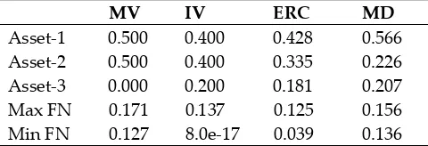
Figure 1. Frobenius norm between true and estimated weights; first row reports misspecification in
326
variance, while second row in covariance. The surfaces’ three dimensions are: the shrinkage intensity
327
in y axis (from 0 to 1); the misspecification in the variance (from 0 to 0.5) or in the covariance (from 0
328
to 1) in x axis and the Frobenius norm in z axis. Each column refers to a specific risk-based portfolio.
329
From the left to the right: MV, IV, ERC, MD, respectively.
330
Moving to the core of this numerical illustration, we proceed as follows. First, for what is
331
concerning the volatility, we let Τ,/ to vary between 0 and 0.5, ceteris paribus. Results are
332
summarised in Figure 1, row 1. As expected, there is no misspecification in all the risk-based portfolio
333
at the initial state Τ,/ = 0.1414, i.e. the true value. All the portfolio weights are misspecified in the
334
range [0; 0.1414), with MV showing the greatest departure from the true portfolio weights when the
335
Asset-3 volatility is undervalued below 0.12. The absence of misspecification effects in the MV
336
weights is due to the initial high-risk attributed to Asset-3: in fact, it is already excluded from the
337
optimal allocation at the initial non-perturbated state. The IV, ERC and MD portfolio weights show
338
nearly the same distance from their not misspecified counterpart. The same applies in the range
339
(0.1414; 0.5], with MD (ERC) showing more (less) misspecification as 0.5 is reached, compared to
340
the others. MV is again not misspecified, since Asset-3 is always excluded from the allocation. This
341
allows the MV portfolio not to be affected by shifts in the shrinkage intensity when there is
over-342
misspecification. On the other hand, the remaining portfolios react in the same way to shrinkage
343
intensity misspecification, showing an increase in the Frobenius norm especially for low values of
344
Asset-3 variance. All the portfolios share the same effect when the weights are estimated with the
345
sample covariance only: in this case the distance from true portfolios is at maximum.
346
Second, we assess the misspecification impact when it arises in the correlation. We let the
347
correlation between Asset-3 and 2 (Ρ; , ) to vary from 0 to 1, ceteris paribus. In this case, we have
348
signs of perturbation in the MV and the MD portfolios, while the ERC shows far less distortion, as
349
presented in Figure 1, row 2. Surprisingly, the IV is not to impacted at all by misspecification in the
350
correlation structure of the target matrix T. Moreover, IV is also the only one not be impacted by the
351
shrinkage intensity misspecification. Both effects are due to the specific characteristics of Asset-3 and
352
the way in which IV selects to allocate weights under a risk-parity scheme. Lastly, MV and ERC show
353
the greatest distortion and hence higher distance from the true weights for small values of shrinkage
354
intensity, while for the MD the Frobenius norm attains its maximum when the target matrix is the
355
estimator (𝛿 = 1).
356
In conclusion, we started this numerical illustration to assess the effects of target matrix
357
misspecification in risk-based portfolios: as in (Ardia et al. 2017), the four risk-based portfolios reacts
similarly to perturbation in volatility and correlation (even if for us they originate in the target
359
matrix), with the MV being the most affected when the variance is misspecified and the IV being the
360
less affected from covariance shifts. In particular, MV performs very poorly when Asset-3 volatility
361
tends to zero. This portfolio is less sensitive to overvalued variance misspecification in very risky
362
assets, but very sensitive in the opposite sense, and it is one of the most affected to perturbations in
363
the correlation. The remaining three portfolios react similarly to variance misspecification, while MD
364
shows a similar sensitivity as the MV to perturbation in the correlation. The IV does not show any
365
sign of distortion when covariance is shifted. Moreover, we improve previous findings showing how
366
weights are affected by shifts in the shrinkage intensity: when sample covariance is the estimator (𝛿 =
367
0), the distance from the true weights stands at maximum level.
368
4. Case Study – Monte Carlo Analysis
369
This section offers a comprehensive comparison of the six target matrix estimators by mean of
370
an extensive Monte Carlo (MC) study. The aim of this analysis is twofold: (i) assessing estimators’
371
statistical properties and similarity with the true target matrix; (ii) addressing the problem of how
372
selecting a specific target estimator impacts on the portfolio weights. This investigation is aimed at
373
giving a very broad overview about (i) and (ii) since we monitor both the 𝑝/𝑛 ratio and the whole
374
spectrum of shrinkage intensity. We run simulations for 15 combinations of 𝑝 and 𝑛, and for 11
375
different shrinkage intensities spanning in the interval [0 ; 1], for an overall number of 165 scenarios.
376
The MC study is designed as follows. Returns are simulated assuming a factor model is the data
377
generating process, as in (MacKinlay and Pastor 2000). In details, we impose a one-factor structure
378
for the returns generating process:
379
380
𝑟 = 𝜉. 𝑓 + 𝜀 ;
381
𝑤𝑖𝑡ℎ 𝑡 = 1, … , 𝑛
382
383
where 𝑓 is the 𝑘 × 1 vector of returns on the factor, 𝜉 is the 𝑝 × 1 vector of factor loadings
384
and 𝜀 the vector of residuals of 𝑝 length. Under this framework returns are simulated implying
385
multivariate normality and absence of serial correlation. The asset factor loadings are drawn from a
386
uniform distribution and equally spread, while returns on the single factor are generated from a
387
Normal distribution. The bounds for the uniform distribution and the mean and the variance for the
388
Normal one are calibrated on real market data, specifically on the empirical dataset “49-Industry
389
portfolios” with monthly frequency, available at Kennet French website5. Residuals are drawn from
390
a uniform distribution in the range [0.10; 0.30] so that the related covariance matrix is diagonal with
391
an average annual volatility of 20%.
392
For each of the 165 scenarios, we apply the same strategy. First, we simulate the 𝑛 × 𝑝 matrix
393
of asset log-returns, then we estimate the six target matrices and their corresponding shrunk matrices
394
Σ . At last, we estimate the weights of the four risk-based portfolios. Some remarks are needed. First,
395
we consider the number of assets as 𝑝 = 10,50,100 and number of observations as 𝑛 =
396
60,120,180,3000,6000 months, which correspond to 5, 10, 15, 250 and 500 years. Moreover, the
397
shrinkage intensity is let to vary between their lower and upper bounds as 𝛿 =
398
0,0.1,0.2,0.3,0.4,0.5,0.6,0.7,0.8,0.9,1 . For each of the 165 scenarios we run 100 Monte Carlo trials6,
399
giving robustness to the results.
400
We stress again the importance of Monte Carlo simulations, which allow us to impose the true
401
covariance Σ and hence the true portfolio weights 𝝎. This is crucial because we can compare the
402
true quantities with their estimated counterparts.
403
5 http://mba.tuck.dartmouth.edu/pages/faculty/ken.french/data_library.html
6 Simulations were done in MATLAB setting the random seed generator at its default value, thus ensuring the
With respect to the point (i), we use two criteria to assess and compare the statistical properties
404
of target matrices: the reciprocal 1-norm condition number (RCN) and the Frobenius Norm. Being
405
the 1-norm condition number (CN) defined as:
406
407
𝐶𝑁(𝐴) = 𝜅(𝐴) = ‖𝐴 ‖,
408
409
for a given A. It measures the matrix sensitivity to changes in the data: when is large, it indicates that
410
a small shift causes important changes, offering a measure of the ill-conditioning of A. Since CN takes
411
value in the interval [0 ; +∞), it is more convenient to use its scaled version, the RCN:
412
413
𝑅𝐶𝑁 = 1/ 𝜅(𝐴). (12)
414
It is defined in the range [0 ; 1]: the matrix is well-conditioned if the reciprocal condition number
415
is close to 1 and ill-conditioned vice-versa. Under the Monte Carlo framework, we will study its MC
416
estimator:
417
418
𝐸[𝐶𝑁] = 1
𝑀 𝐶𝑁 , (13)
419
where 𝑀 is the number of MC simulations. On the other hand, the Frobenius norm is employed to
420
gauge the similarity between the estimated target matrix and the true one. We define it for the 𝑝 × 𝑝
421
symmetric matrix 𝑍 as:
422
423
𝐹𝑁(𝑍) = ‖𝑍‖ = 𝑧 .
424
425
In our case, 𝑍 = Σ − Σ. Its Monte Carlo estimator is given by the following
426
427
𝐸[𝐹𝑁] = 1
𝑀 𝐹𝑁 . (14)
428
Regarding (ii), we assess the discrepancy between true and estimated weights again with the
429
Frobenius norm. In addition, we report the values at which the Frobenius norm attains its best results,
430
i.e. when the shrinkage intensity is optimal.
431
432
4.1. Main Results
433
434
Figure 2 summarises the statistical properties of the various target matrices.
436
Figure 2. The condition number (y-axis) as the 𝑝/𝑛 ratio moves from 60𝑝 to 6000𝑝 . Each column
437
corresponds to a specific target matrix: from left to right, the Identity, the Variance Identity, the
Single-438
Index, the Common Covariance, the Constant Correlation and the EWMA, respectively. Each row
439
corresponds to a different 𝑝: in ascendant order from 10 (first row) to 100 (third row).
440
441
442
443
The Figure 2 shows from left to right the condition numbers for the Identity, the Variance Identity,
444
the Market model, the Common Variance, the Constant Correlation and the EWMA, respectively.
445
Each column corresponds to a specific target, while each rows refer to a different number of assets
446
𝑝: the first column to 10, the secondo to 50 and the third to 100. For each sub-figure, on the x-axis we
447
show the 𝑝/𝑛 ratio in ascendant order and on the y-axis the condition number: the matrix is
well-448
conditioned when its value is closer to 1, vice-versa is ill-conditioned the more it tends zero.
449
Figure 3. Surfaces representing the Frobenius norm (z-axis) between the true and the estimated target
450
matrices, considering the shrinkage intensity (y-axis) and the 𝑝/𝑛 ratio (x-axis). Each column
451
corresponds to a specific target matrix: from left to right, the Identity, the Variance Identity, the
Single-452
Index, the Common Covariance, the Constant Correlation and the EWMA, respectively. Each row
453
corresponds to a different 𝑝: in ascendant order from 𝑝 = 10 (first row) to 𝑝 = 100 (third row).
Then, we turn to the study of similarity among true and estimated target matrices. Figure 3
455
represents the Monte Carlo Frobenius norm between the true and the estimated target matrices. The
456
surfaces give a clear overview about the relation among the Frobenius norm itself, the 𝑝/𝑛 ratio and
457
the shrinkage intensity. Overall, the Frobenius norm is minimised by the Single-Index and the CC: in
458
these cases the target matrices are not particularly affected by the shrinkage intensity, while their
459
reaction to increases in the 𝑝/𝑛 ratio are controversial. In fact, quite surprisingly the distance
460
between true and estimated weights diminishes as both 𝑝 and 𝑛 increases. For 𝑝 = 50 and 𝑝 = 100
461
there is a hump for small 𝑝/𝑛 values; however, the Frobenius norm increases when ≥ 1. Despite
462
of the low condition number, the EWMA shows a similar behaviour to the Single-Index and the
463
Constant Correlation target matrices, especially w.r.t. 𝑝/𝑛 values. On the other hand, it is more
464
affected by shifts in the shrinkage parameters; the distance from the true weights increases moving
465
towards the target matrix. Lastly, the Common Covariance and the Variance Identity are very far
466
away from the true target matrix: they are very sensitive to high 𝑝/𝑛 and 𝛿 values.
467
To conclude, the identity is the most well-conditioned matrix, and it is stable across all the
468
examined 𝑝/𝑛 combinations. Nevertheless, the Single-Index and the CC target matrices show the
469
greater similarity with the true target matrix minimizing Frobenius norm, while the identity seems
470
less similar to the true target.
471
472
4.1.1. Results on Portfolio Weights
473
Table 3 and Table 4 present main results of the Monte Carlo study: for each combination of 𝑝
474
and 𝑛, we report the Monte Carlo estimator of the Frobenius norm between true and estimated
475
weights. In particular, Table 3 reports averaged Frobenius norm along the shrinkage intensity
476
(excluding the case 𝛿 = 0, which corresponds to the sample covariance matrix), while Table 4 lists
477
the minimum values for the optimal shrinkage intensity.
Table 3. Frobenius norm for the portfolio weights. Values are averaged along the shrinkage intensity
504
(excluding the case 𝛿 = 0). For each 𝑛, the first line reports the Frobenius norm for the sample
505
covariance matrix. Abbreviations in use are: S for sample covariance; Id for identity matrix; Vid for
506
Variance Identity; SI for Single-Index; CV for Common Covariance; CC for Constant Correlation and
507
EWMA for Exponentially Weighted Moving Average.
508
P=10 P=50 P=100
MV IV ERC MD MV IV ERC MD MV IV ERC MD
Panel A: n=60
S 0.834 0.1585 0.1736 0.5842 0.7721 0.0573 0.0637 0.4933 0.7555 0.0409 0.0447 0.4565 Id 0.6863 0.1425 0.1528 0.5045 0.6215 0.0559 0.0631 0.3873 0.4967 0.0404 0.0451 0.3652
VId 0.6935 0.1583 0.1732 0.5176 0.5999 0.0567 0.0634 0.4092 0.5901 0.0404 0.0445 0.3686
SI 0.838 0.1585 0.1736 0.5678 0.7685 0.0573 0.0637 0.4709 0.75 0.0409 0.0447 0.4288
CV 1.2438 0.1583 0.1731 1.011 1.1484 0.0567 0.0628 0.9381 1.1386 0.0404 0.0438 0.9185 CC 0.8353 0.1585 0.1733 0.5361 0.7808 0.0573 0.0635 0.4328 0.7663 0.0409 0.0445 0.3922 EWMA 0.8473 0.1593 0.1745 0.595 0.7811 0.0575 0.064 0.5142 0.7325 0.0411 0.045 0.4431
Panel B: n=120
S 0.9064 0.0877 0.0989 0.4649 0.7814 0.059 0.0656 0.5065 0.6519 0.0424 0.0472 0.4332 Id 0.8157 0.087 0.0983 0.4256 0.6259 0.0613 0.0688 0.4354 0.6307 0.0389 0.0431 0.328
VId 0.8235 0.0871 0.0985 0.4284 0.6259 0.0613 0.0688 0.4354 0.489 0.0421 0.0471 0.3712
SI 0.9097 0.0877 0.0989 0.4563 0.7777 0.059 0.0656 0.4925 0.6458 0.0424 0.0472 0.419 CV 1.3269 0.0871 0.0982 0.9667 1.1806 0.0587 0.0651 1.0138 1.0974 0.0421 0.0467 0.8951 CC 0.905 0.0877 0.0988 0.4357 0.7822 0.059 0.0655 0.4636 0.6566 0.0424 0.0471 0.3856 EWMA 0.9281 0.0883 0.0996 0.4859 0.7994 0.0592 0.0658 0.5246 0.6788 0.0427 0.0475 0.4601
Panel C: n=180
S 0.7989 0.1311 0.1423 0.5007 0.7932 0.0564 0.0627 0.4631 0.6905 0.0404 0.044 0.4065 Id 0.7206 0.1308 0.142 0.4736 0.6705 0.0562 0.0625 0.405 0.5477 0.0375 0.0399 0.3748
VId 0.7273 0.1308 0.1421 0.4757 0.6838 0.0562 0.0626 0.4127 0.5754 0.0402 0.044 0.3556
SI 0.8001 0.1311 0.1423 0.4954 0.7904 0.0564 0.0627 0.4545 0.6873 0.0404 0.044 0.3982 CV 1.2715 0.1308 0.1419 0.9961 1.2073 0.0562 0.0624 0.9988 1.1422 0.0402 0.0437 0.8705
CC 0.7957 0.1311 0.1423 0.4803 0.792 0.0564 0.0626 0.4259 0.692 0.0404 0.044 0.3672
EWMA 0.8415 0.1322 0.1435 0.526 0.8284 0.0567 0.0631 0.5005 0.7206 0.0408 0.0445 0.4429
Panel D: n=3000
S 0.7504 0.1476 0.1596 0.3957 0.734 0.049 0.0539 0.3988 0.513 0.0384 0.0428 0.3259
Id 0.7441 0.1477 0.1597 0.3946 0.7009 0.049 0.0539 0.3872 0.4615 0.0384 0.0428 0.3096
VId 0.7437 0.1477 0.1596 0.3945 0.7043 0.049 0.0539 0.3886 0.4673 0.0384 0.0428 0.312
SI 0.7516 0.1476 0.1596 0.3955 0.7339 0.049 0.0539 0.3984 0.5123 0.0384 0.0428 0.3252 CV 1.2864 0.1477 0.1597 0.963 1.2281 0.049 0.0538 0.9954 1.1041 0.0384 0.0428 0.6822 CC 0.7488 0.1476 0.1596 0.3949 0.7316 0.049 0.0539 0.3904 0.5096 0.0384 0.0428 0.3143 EWMA 0.8563 0.1489 0.1611 0.4452 0.8161 0.0497 0.0547 0.4652 0.6244 0.0389 0.0435 0.4076
Panel E: n=6000
S 0.9672 0.1302 0.1409 0.4821 0.5737 0.0539 0.0589 0.3481 0.5772 0.0402 0.0437 0.3436 Id 0.9496 0.1301 0.1408 0.4813 0.6095 0.0575 0.0639 0.4076 0.5449 0.0402 0.0437 0.3342
VId 0.951 0.1301 0.1409 0.4815 0.5419 0.054 0.0589 0.3401 0.5483 0.0402 0.0437 0.3354
SI 0.9688 0.1302 0.1409 0.482 0.574 0.0539 0.0589 0.3479 0.5772 0.0402 0.0437 0.3434 CV 1.4142 0.1301 0.1408 1.0034 1.1436 0.054 0.0589 0.9706 1.1422 0.0402 0.0437 0.7031 CC 0.9656 0.1302 0.1409 0.4814 0.5709 0.0539 0.0589 0.3415 0.575 0.0402 0.0437 0.3368 EWMA 1.0432 0.1312 0.1422 0.5232 0.6946 0.0547 0.0599 0.4319 0.681 0.0407 0.0444 0.4229
509
In both tables, we compare the six target matrices by examining one risk-based portfolio at time
510
and the effect of increasing 𝑝 for fixed 𝑛. Special attention is devoted to the cases when 𝑝 > 𝑛: the
511
high-dimensional sample. We have this scenario only when 𝑝 = 100 and 𝑛 = 60. Here, the sample
covariance matrix becomes ill-conditioned (Marčenko and Pastur 1967), thus it is interesting to
513
evaluate gains obtained with shrinkage. The averaged Frobenius norm values in Table 3 give us a
514
general overview about how target matrices perform across the whole shrinkage intensity spectrum
515
in one goal. We aim to understand if, in average terms, shrinking the covariance matrix benefits
risk-516
portfolio weights. On the other hand, the minimum Frobenius norm values help us understanding
517
to what extent the various target matrices can help reproducing the true portfolio weights: the more
518
intensity we need, the better is the target. In both tables, sample values are listed in the first row of
519
each Panel.
520
Starting from Table 3, Panel A, the MV allocation seems better described by the Identity and the
521
Variance Identity regardless the number of assets 𝑝. In particular, we look at the difference between
522
the weights calculated entirely on the sample covariance matrix and the those of the targets: the
523
Identity and the Variance Identity are the only estimator to perform better. In fact, shrinking towards
524
the sample is not as bad as shrinking towards the Common Covariance. Increasing 𝑛 and moving
525
to Panel B, similar results are obtained. This trend is confirmed in Panel C, while in the cases of 𝑛 =
526
3000 and 𝑛 = 6000 all the estimators perform similarly. Hence, for the MV portfolio the Identity
527
matrix works at best in reproducing portfolio weights very similar to the true ones. The same
528
conclusions applies for the MD portfolio: when 𝑝 and 𝑛 are small, the Identity and the Variance
529
Identity overperform other alternatives. On the other hand, we get very different results for the IV
530
and ERC. Both portfolios seem not gaining benefits from the shrinkage procedure, as the Frobenius
531
norm is very similar to that of the sample covariance matrix for all the target matrices under
532
consideration. This is true for all pairs of 𝑝 and 𝑛. In the high-dimensional case (𝑝 = 100; 𝑛 = 60)
533
the Identity matrix works best in reducing the distance between true and estimated portfolio weights,
534
both for the MV and MD portfolios. In average, shrinkage does not help too much when alternative
535
target matrices are used; only in the case of Common Covariance shrinking is worse than using the
536
sample covariance matrix. All these effects vanish when we look at the IV and ERC portfolios: here,
537
shrinkage does not help too much, whatever the target is.
538
Overall, the results are in line with the conclusions of the numerical illustrations in Section 3.
539
Indeed, the MV portfolio shows the highest distance between true and estimated weights, similarly
540
to the MD. Both portfolios are affected by the dimensionality of the sample: shrinkage always help
541
in reducing weights misspecification; it improves in high-dimensional cases. On contrary, estimated
542
weights for the IV and the ERC portfolios are close to the true ones by construction, hence, shrinkage
543
does not help too much.
544
Switching to Table 4, results illustrate again the Identity and the Variance Identity attaining the best
545
reduction of the Frobenius norm for the MV and MD portfolios. If results are similar to those of Table
546
3 for the MV, results for the MD show an improvement in using the shrinkage estimators. The
547
Identity, Variance Identity, Common Covariance and Constant Correlation target matrices
548
overperform all the alternatives, including the sample estimator, minimising the Frobenius norm in
549
a similar fashion. This is true also for the high-dimensional case. On the contrary, the IV and the ERC
550
do not benefit from shrinking the sample covariance matrix, even in high-dimensional samples,
551
confirming Table 3 insights. Lastly, we look at the shrinkage intensity at which target matrices attain
552
the highest Frobenius norm reduction. The intensity is comprised in the interval [0; 1]: the more it is
553
close to 1, the more the target matrix helps in reducing the estimation error of the sample covariance
554
matrix. interestingly, the Identity and the Variance Identity show shrinkage intensities always close
555
to 1, meaning that shrinking towards them is highly beneficial, as they are fairly better than the
556
sample covariance matrix. This is verified either for the high-dimensional case and for those risk
557
portfolios (IV and ERC) who do not show great improvements from shrinkage.
558
Table 4. Frobenius norm for the portfolio weights. Values corresponds to the optimal shrinkage
559
intensity, listed after the Frobenius norm for each portfolio. We report values for the sample
560
covariance matrix (𝛿 = 0) separately in the first row of each panel. For each 𝑛, the first line reports
561
the Frobenius norm for the sample covariance matrix. Abbreviations stand for: S for sample
562
covariance; Id for identity matrix; VId for Variance Identity; SI for Single-Index; CV for Common
563
Covariance; CC for Constant Correlation and EWMA for Exponentially Weighted Moving Average.
P=10 P=50 P=100
MV IV ERC MD MV IV ERC MD MV IV ERC MD
Panel A: n=60
S 0.834 0 0.1585 0 0.1736 0 0.5842 0 0.7721 0 0.0573 0 0.0637 0 0.4933 0 0.7555 0 0.0409 0 0.0447 0 0.4565 0
Id 0.6778 0.7 0.1424 0.4 0.1525 0.8 0.501 0.8 0.5997 1 0.0558 1 0.0624 1 0.3704 1 0.471 1 0.0403 0.8 0.0446 1 0.3462 1
VId 0.6689 0.9 0.1581 0.5 0.173 0.9 0.5084 0.9 0.5539 1 0.0565 0.9 0.0627 1 0.3795 1 0.5428 1 0.0402 1 0.0437 1 0.3331 1
SI 0.8345 0.1 0.1585 0.1 0.1735 1 0.558 1 0.7666 1 0.0573 0.1 0.0637 0.1 0.4633 0.9 0.7479 1 0.0409 0.1 0.0447 0.1 0.4195 0.9
CV 1.2392 0.1 0.1581 0.5 0.1729 0.2 0.509 1 1.117 0.1 0.0565 0.9 0.0627 0.5 0.3795 1 1.1068 0.1 0.0402 1 0.0437 1 0.3331 1
CC 0.8335 0.3 0.1585 0.1 0.1731 1 0.5081 1 0.7733 0.1 0.0573 0.1 0.0634 1 0.3795 1 0.757 0.1 0.0409 0.1 0.0444 1 0.3332 1
EWMA 0.8331 0.1 0.1586 0.1 0.1737 0.1 0.5852 0.1 0.7706 0.1 0.0573 0.1 0.0637 0.1 0.4953 0.1 0.7213 1 0.0409 0.1 0.0447 0.1 0.4395 0.6
Panel B: n=120
S 0.9064 0 0.0877 0 0.0989 0 0.4649 0 0.7814 0 0.059 0 0.0656 0 0.5065 0 0.6519 0 0.0424 0 0.0472 0 0.4332 0
Id 0.8121 0.6 0.087 0.6 0.0981 0.8 0.4241 0.7 0.6119 1 0.0613 0.9 0.0685 1 0.4255 1 0.613 1 0.0388 0.9 0.0428 1 0.3111 1
VId 0.8121 0.8 0.087 0.8 0.0982 0.9 0.4242 0.9 0.6119 1 0.0613 0.9 0.0685 1 0.4255 1 0.4425 1 0.042 1 0.0467 1 0.3445 1
SI 0.907 0.1 0.0877 0.1 0.0989 1 0.4526 1 0.776 1 0.059 0.1 0.0656 1 0.4872 1 0.6431 1 0.0424 0.1 0.0472 0.1 0.414 0.9
CV 1.3269 0.1 0.087 0.8 0.0981 0.3 0.4245 1 1.1756 0.1 0.0586 0.9 0.0651 0.5 0.4302 1 1.0916 0.1 0.042 1 0.0467 1 0.3445 1
CC 0.9043 0.8 0.0877 0.1 0.0987 1 0.4241 0.9 0.781 0.2 0.059 0.2 0.0654 1 0.4302 1 0.6527 0.1 0.0424 0.1 0.0471 1 0.3446 1
EWMA 0.9052 0.1 0.0876 0.2 0.0988 0.2 0.4651 0.1 0.7797 0.2 0.0589 0.2 0.0655 0.2 0.5056 0.1 0.6554 0.1 0.0424 0.1 0.0472 0.1 0.4331 0.1
Panel C: n=180
S 0.7989 0 0.1311 0 0.1423 0 0.5007 0 0.7932 0 0.0564 0 0.0627 0 0.4631 0 0.6905 0 0.0404 0 0.044 0 0.4065 0
Id 0.7177 0.5 0.1307 0.7 0.1419 0.9 0.4724 0.8 0.6613 0.8 0.0562 0.6 0.0624 1 0.3977 0.9 0.534 1 0.0375 0.6 0.0398 1 0.3645 1
VId 0.718 0.7 0.1307 0.9 0.1419 1 0.4724 0.9 0.6614 0.9 0.0562 0.8 0.0624 1 0.3979 1 0.5428 1 0.0402 1 0.0437 1 0.3331 1
SI 0.799 0.2 0.1311 0.1 0.1423 1 0.4929 1 0.7897 0.7 0.0564 0.1 0.0627 1 0.4515 0.9 0.6863 0.8 0.0404 0.1 0.044 1 0.3955 0.8
CV 1.2715 0.1 0.1307 0.9 0.1418 0.4 0.4724 1 1.2073 0.1 0.0562 0.8 0.0624 0.4 0.3979 1 1.1422 0.1 0.0402 1 0.0437 0.9 0.3331 1
CC 0.7942 1 0.1311 0.1 0.1422 1 0.4725 1 0.7912 0.4 0.0564 0.1 0.0626 1 0.3977 1 0.6904 0.1 0.0404 0.1 0.0439 1 0.3331 1
EWMA 0.8035 0.1 0.1312 0.1 0.1424 0.1 0.5008 0.1 0.7951 0.1 0.0564 0.1 0.0626 0.1 0.4653 0.1 0.6938 0.1 0.0404 0.1 0.044 0.1 0.4074 0.1
Panel D: n=3000
S 0.7504 0 0.1476 0 0.1596 0 0.3957 0 0.734 0 0.049 0 0.0539 0 0.3988 0 0.513 0 0.0384 0 0.0428 0 0.3259 0
Id 0.7425 0.1 0.1477 0.1 0.1596 0.1 0.3941 0.1 0.6988 1 0.049 1 0.0538 1 0.3859 1 0.4573 1 0.0384 1 0.0428 1 0.3072 1
VId 0.7426 0.3 0.1476 0.1 0.1596 0.1 0.3941 0.3 0.6988 1 0.049 1 0.0538 1 0.3859 1 0.4573 1 0.0384 1 0.0428 1 0.3072 1
SI 0.7506 0.1 0.1476 0.1 0.1596 0.1 0.3953 1 0.7339 0.5 0.049 0.1 0.0539 1 0.3983 0.8 0.512 1 0.0384 0.2 0.0428 1 0.325 0.9
CV 1.2864 0.1 0.1476 0.1 0.1596 0.1 0.3951 1 1.2281 0.1 0.049 1 0.0538 1 0.3859 1 1.1041 0.1 0.0384 1 0.0428 1 0.3072 1
CC 0.7477 1 0.1476 0.1 0.1596 0.1 0.3946 0.7 0.7299 1 0.049 0.1 0.0539 1 0.386 1 0.5073 1 0.0384 0.2 0.0428 1 0.3072 1
EWMA 0.7615 0.1 0.1477 0.1 0.1597 0.1 0.3981 0.1 0.7439 0.1 0.0491 0.1 0.0539 0.1 0.4043 0.1 0.5263 0.1 0.0384 0.1 0.0429 0.1 0.3346 0.1
Panel E: n=6000
S 0.9672 0 0.1302 0 0.1409 0 0.4821 0 0.5737 0 0.0539 0 0.0589 0 0.3481 0 0.5772 0 0.0402 0 0.0437 0 0.3436 0
Id 0.9486 1 0.13 1 0.1408 1 0.4811 1 0.6085 0.7 0.0575 0.1 0.0639 0.1 0.4072 0.8 0.5428 1 0.0402 1 0.0437 1 0.3331 1
VId 0.9486 1 0.13 1 0.1408 1 0.4811 1 0.5365 1 0.054 0.1 0.0589 0.7 0.3381 1 0.5428 1 0.0402 1 0.0437 1 0.3331 1
SI 0.9675 0.1 0.1302 0.1 0.1409 1 0.482 1 0.5738 0.1 0.0539 0.1 0.0589 1 0.3478 1 0.5772 0.4 0.0402 0.1 0.0437 1 0.3433 0.8
CV 1.4142 0.1 0.13 1 0.1408 1 0.4811 1 1.1436 0.1 0.054 0.1 0.0589 0.1 0.3381 1 1.1422 0.1 0.0402 1 0.0437 1 0.3331 1
CC 0.9644 1 0.1302 0.1 0.1409 1 0.4812 1 0.5687 1 0.0539 0.1 0.0589 1 0.3381 1 0.5733 1 0.0402 0.9 0.0437 1 0.3331 1
EWMA 0.9765 0.1 0.1302 0.1 0.1409 0.1 0.4832 0.1 0.5901 0.1 0.054 0.1 0.059 0.1 0.3561 0.1 0.59 0.1 0.0402 0.1 0.0438 0.1 0.3524 0.1
4.2.3 Sensitivity to shrinkage intensity
566
567
To have a view on the whole shrinkage intensity spectrum (i.e. the interval [0; 1]) we refer to
568
Figure 3, where we report the Frobenius Norms for the weights (y-axis) w.r.t. the shrinkage intensity
569
(x-axis). Each column corresponds to a specific risk-based portfolio: from left to right, the Minimum
570
Variance, the Inverse Volatility, the Equal-Risk-Contribution and the Maximum Diversification,
571
respectively. Each row corresponds to the 𝑝/𝑛 ratio in 𝑛 ascending order. For each subfigure, the
572
Identity is blue o-shaped, the Variance Identity is green square-shaped, the Single-Index is red
573
hexagram-shaped, the Common Covariance is black star-shaped, the Constant Correlation is cyan
+-574
shaped and the EWMA is magenta diamond-shaped.
575
576
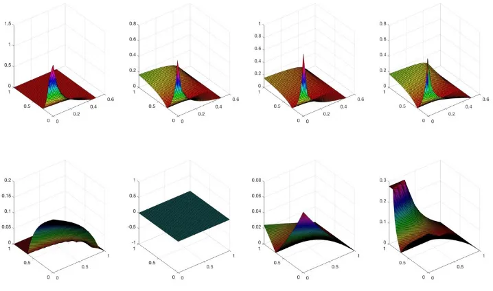
Figure 4. Frobenius norm for portfolio weights with respect to the shrinkage parameter, when 𝑝 =
577
100.
578
Figure 4 illustrates the case 𝑝 = 100, so to include the high-dimensional scenario. Starting from
579
the latter (first row, 𝑛 = 60), the Variance Identity is the only target matrix to always reduce weight
580
misspecification for all the considered portfolios, for all shrinkage levels. The Identity do the same,
581
excluding the ERC case where it performs worse than the sample covariance matrix. the remaining
582
targets behave very differently across the four risk-based portfolios: the Common Covariance is the
583
worst in both the MV and MD and the EWMA is the worst in both ERC and IV. The Market Model
584
and the Constant Correlation do not improve much from the sample estimator across all portfolios.
585
Looking at the second row (𝑛 = 120), the Identity is the most efficient target, reducing the
586
distance between estimated and true portfolio weights in all the considered portfolios. The Variance
587
Identity is also very efficient in MV and MD portfolios, while the remaining targets show similar
588
results as in the previous case. The same conclusions apply for the case 𝑛 = 180.
589
When the number of observations is equal or higher than 𝑛 = 3000, results do not change much.
590
The Identity, the Variance Identity, the Market model and the Constant Correlation are the most
591
efficient target matrices towards to shrink, while the EWMA is the worst for both IV and ERC
592
portfolios and the Common Covariance is the worst for the MV and MD ones.
593
In conclusion, for the MV portfolio the Common Covariance should not be used, since it always
594
produces weights very distant from the true ones being very unstable. At the same time, the EWMA
595
should not be used to shrink the covariance matrix in the IV and ERC portfolios. The most convenient