Improving Galvanizing Bath Hardware

(1)

Scholarship@Western

Electronic Thesis and Dissertation Repository

May 2015

Improving Galvanizing Bath Hardware

Amir Kargar Neghab Supervisor

Dr. Andrew Hrymak

The University of Western Ontario

Graduate Program in Chemical and Biochemical Engineering

A thesis submitted in partial fulfillment of the requirements for the degree in Master of Engineering Science

Follow this and additional works at: https://ir.lib.uwo.ca/etd

Part of the Engineering Commons

Recommended Citation Recommended Citation

Kargar Neghab, Amir, "Improving Galvanizing Bath Hardware" (2015). Electronic Thesis and Dissertation Repository. 2814.

https://ir.lib.uwo.ca/etd/2814

This Dissertation/Thesis is brought to you for free and open access by Scholarship@Western. It has been accepted for inclusion in Electronic Thesis and Dissertation Repository by an authorized administrator of

(2)

(Thesis format: Monograph)

by

Amir Kargar Neghab

Graduate Program in Chemical and Biochemical Engineering

A thesis submitted in partial fulfillment of the requirements for the degree of

Masters of Engineering Science

The School of Graduate and Postdoctoral Studies The University of Western Ontario

London, Ontario, Canada

(3)

ii

Abstract

Suspended dross particles in galvanizing bath can interact with moving rolls that guide the strip

and eventually accumulate on it. They can cause the roll to function improperly and reduce the

surface quality of galvanized steel sheet.

In this research, a turbulent flow simulation of a continuous sheet galvanizing bath is carried

out using the computational fluid mechanics in Ansys FLUENT to determine the flow profile

inside a galvanizing bath. Multiphase flow modeling has been performed to understand the

particle-surface interactions by coupling the particulate models for solid phase with

computational fluid dynamics for fluid phase.

A strong fluid flow along the roll axis, which captures a significant number of dross particles,

was found in the 3D bath simulation. It was observed that surface region in which particles

agglomerate on the roll reported by the industry is the same as where particles collisions with

the roll were observed in the simulation.

Keywords

(4)

iii

Acknowledgments

I would like to extend my gratitude to the many people who helped me to complete this research

project.

Foremost, I would like to sincerely thank my advisor, Dr. Andrew Hrymak for his continual

supervision and guidance throughout my program and for providing me the opportunity of

obtaining a graduate degree at Chemical Engineering Department at Western University.

I am also grateful for valuable assistance and financial support of Dr. Frank Goodwin and

International Lead Zinc Organization throughout this research project. I would also like to

acknowledge the guidance of Professor Anthony Straatman and the valuable questions he

raised. I sincerely thank the examination committee Dr. Mita Ray and Dr. Cedric Briens.

Special thanks to my supportive and caring wife, Mehraneh for giving me the motivation and

confidence and also my parents, my sisters and my in-laws for their faith and continuous

support. Lastly, I would like to thank my best friends and intellectual partners Ethan Doan and

(5)

iv

List of Tables

Table 4- 1: Configuration and operating conditions ... 17

Table 4- 2: Parameters used for the CFD study of liquid phase ... 24

Table 4- 3: Parameters used for the DPM and DEM studies of solid phase ... 37

Table 5- 1: Boundary types and conditions data ... 49

Table 6- 1: Correlation between critical velocity, surface tension and viscosity ... 61

(9)

viii

List of Figures

Figure 1- 1: Continuous hot-dip galvanizing line ... 2

Figure 1- 2: Geometry of galvanizing bath ... 3

Figure 4- 1: Geometry of the studied galvanized bath ... 16

Figure 4- 2: Surface elements in the galvanizing bath ... 18

Figure 4- 3: Cross section of the initial mesh within the bath ... 19

Figure 4- 4: Improved surface elements of the bath hardware components ... 20

Figure 4- 5: Wedge area near the roll ... 20

Figure 4- 6: Cross section of the mesh grid at the middle of the bath ... 21

Figure 4- 7: Close-up view of the mesh grid close to the sink roll ... 22

Figure 4- 8: Displaying the prism layers on the roll and strip surface ... 22

Figure 4- 9: Improvement of volume elements at the wedge area ... 23

Figure 4- 10: Velocity contours inside the galvanizing bath ... 24

Figure 4- 11: Displaying of the cut-planes in the bath ... 25

Figure 4- 12: Top view of the defined cut-planes in the bath ... 25

Figure 4- 13: Velocity vectors at the middle of the bath ... 26

Figure 4- 14: Velocity vectors at the X-Z cut-plane ... 27

Figure 4- 15: Velocity contours at the X-Z cut-plane ... 27

Figure 4- 16: A close-view of the velocity vectors at the X-Z cut-plane ... 27

(10)

ix

Figure 4- 19: Fluid flow direction at the wedge area ... 29

Figure 4- 20: Locations for particle injections in the galvanizing bath ... 38

Figure 4- 21: Injection 1- From snout region in front of the strip ... 39

Figure 4- 22: Injection 2-From top of the sink roll ... 39

Figure 4- 23: DPM Particle trajectory for a particle close to the middle of the roll ... 40

Figure 4- 24: DPM Particle trajectory for a particle closer to strip edge ... 40

Figure 4- 25: DPM Particle trajectory for single particle released from strip edge ... 40

Figure 4- 26: DPM massless-particle trajectory at middle of the roll... 41

Figure 4- 27: DPM massless particle trajectory for a particle closer to the strip edge ... 41

Figure 4- 28: DPM massless particle trajectory for a particle at the strip edge ... 41

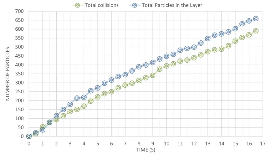
Figure 4- 29: Defined layer around the sink roll ... 42

Figure 4-30: Cumulative number of particles at the extreme vicinity of the roll ... 43

Figure 5- 1: Groove geometry details ... 46

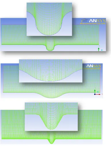
Figure 5- 2: Mesh grid for geometry 1, 2 and 3, from top to bottom ... 48

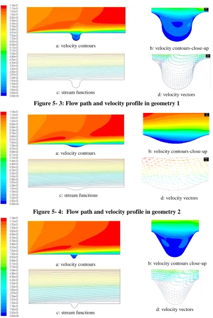
Figure 5- 3: Flow path and velocity profile in geometry 1 ... 50

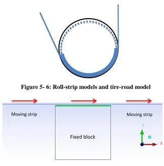
Figure 5- 6: Roll-strip models and tire-road model ... 51

(11)

x

Figure 5- 9: 3D strip-block geometry 2 ... 52

Figure 5- 10: Velocity profile at the entrance of the nip area- δ=1mm ... 53

Figure 5- 11: Velocity profile at the entrance of the nip area-δ=5mm ... 53

Figure 5- 12: Straight groove in the cavity study- δ=0.25mm ... 54

Figure 5- 13: Tilted groove in the cavity study- δ=0.25mm ... 54

Figure 5- 14: Tilted groove position for θ=7° ... 55

Figure 5- 18: Groove geometry 2- Intersection of 3 circles... 56

Figure 5- 19: Modified geometry ... 57

Figure 5- 20: Velocity Profile for groove angle θ=0° ... 57

Figure 6- 1: Stages leading to air-entrainment ... 60

Figure 6- 2: Bath geometry ... 63

(12)

xi

Figure 6- 5: Volume fraction in the bath at t=0.05s ... 65

Figure 6- 6: Volume fraction at the bath at t=0.29s ... 66

Figure 6- 7: Volume fraction at the bath at t=0.59s ... 66

Figure 6- 8: Fluid behaviour at the meniscus at t=2.78s ... 66

Figure 6- 9: Coating layer formed on the strip ... 67

Figure 6- 10: Liquid velocity vectors on the strip where it leaves the bath ... 67

Figure 6- 11: Liquid velocity vectors for the fluid on top of the roll ... 68

Figure 6- 12: Velocity vectors for the liquid- close to the guide roll ... 69

Figure 6- 13: Liquid velocity vectors for the fluid on top of the roll ... 69

(13)

xii

Nomenclature

Roman Letters

𝐴 particle projected area

𝐶𝑡 tangential dashpot coefficients

CD drag coefficient

𝐶𝜀1, 𝐶𝜀2 , 𝐶𝜇,, 𝜎𝜀 ,𝜎𝑘 model constants

d diameter, m

f body force per unit mass, N/kg

FD drag force N

F_x acceleration force

g gravitational acceleration, m/s2

𝐼 particle moment of inertia

k turbulent kinetic energy, m2/s2

𝐾𝑡 tangential spring coefficients

𝑚 particle mass

P pressure, Pa

Re Reynolds number

t time, s

u velocity, m/s

𝑢_∗ friction velocity

𝑉_𝑐 critical velocity

𝑋 location parameter

𝑌 distance from wall

𝑌+ wall coordinate

Greek Letters

Δ change in a property

∇ gradient

ε dissipation rate, m2_/s3

(14)

xiii

𝜔 particle rotational velocity

𝜏 stress, N/m2

𝜇 static coefficient

𝛿 distance, m

𝜎 surface tension

Subscripts

k turbulent kinetic energy

ε dissipation rate

p particle

f fluid

Abbreviations

DEAL Determining Effective Aluminum

DEM Discrete Element Method

DPM Discrete Particle Method

MAP Modeling Aluminum Pick-up

RANS ReynoldsAveraged Navier Stokes

PIV Particle Image Velocimetry

SWF Standard Wall Function

(15)

Chapter 1

1.1 Introduction

Zinc has been used as one of the most important materials to improve the corrosion

durability and performance of steel. This improvement is provided by the process of

coating of steel. Hot-dip coating has been found to be one of the most economical methods

for steel protection from the corrosion phenomenon.

Galvanized steel sheets are produced in a complex metallurgical process known as

continuous hot-dip galvanizing process. Galvanized steel can be found in almost every

industry that uses steel including utilities, paper industry, household appliances,

construction materials and any other industry where the final products are subject to

outdoor exposure. However, the most important product in the market is the galvanized

steel used in automotive industry. Almost 75% of all galvanized steel sheet is produced for

auto body and the remaining percentage is used for other purposes [1].

Some of the unique properties of galvanized steel are: corrosion resistance, low initial cost,

long life, formability, reliability, recyclability, light weight and high strength.

1.2 Galvanizing Process Description

Continuous hot-dip galvanizing is a complex metallurgical process which involves

continuous submersion of steel sheet in a molten zinc bath resulting in coating of the steel

sheet. Galvanizing process consists of 4 basic steps: surface preparation, Annealing,

galvanizing and inspection. The most critical part in the industrial galvanizing line is where

the actual metallurgical reaction between the steel and the zinc takes place. This study

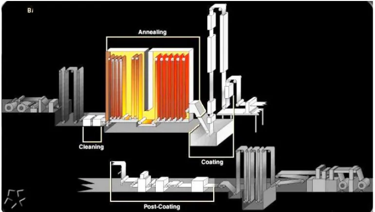
focuses on the galvanizing bath. Figure 1-1 displays a schematic continuous hot-dip

galvanizing line.

In a typical hot-dip galvanizing line [2], the steel strip is first uncoiled and then welded to

the previous sheet coil to keep the production continuous. After the cleaning process in the

pre-treatment section, the strip is rinsed and dried to enter to the furnace to increase its

(16)

Figure 1- 1: Continuous hot-dip galvanizing line

The most critical part in the industrial galvanizing line is where the actual metallurgical

reaction between the steel and the zinc takes place.

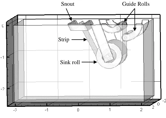
As shown Figure 1-2, a galvanizing bath contains a snout, a sink roll, two guide rolls which

are supported by bearings. In the galvanizing bath, steel is submerged into the molten zinc

at speeds ranging between 1 to 3m/s through snout. The strip speed depends on the design

of the galvanizing line and its application. The steel strip reacts with the molten zinc alloy

at a temperature between 450°C and 480°C to form a protective coating layer on the steel

surface.

Generally, once the strip exits the bath, the excess molten zinc is removed from the strip

by the wiping air knives. Air knives produce high pressure jets of air (or nitrogen gas) to

control the coating thickness. Then the product goes to the post treatment section.

In the galvanizing bath, intermetallic compounds in the form of dross particles are

generated through chemical reactions in the bath. These particles can collide with the bath

hardware components and eventually agglomerate. One of the main reasons for roll failure

is dross build-up on the surface of the sink roll. The main locations of agglomeration

(17)

Figure 1- 2: Geometry of galvanizing bath

This degradation can stop the operation of the galvanizing line and reduce the coating

quality of the steel sheets. Dross build-up increases the maintenance cost and shut down

time for replacement of the defective hardware components. The cost of re-running a

galvanizing line due to failure is roughly estimated to be around $1000 per hour [3] in

addition to loss of production, energy and profit.

1.3 Dross Particle

Isolated intermetallic particles known as dross are generated in the galvanizing bath

through chemical reactions between molten zinc, aluminum, and iron. These particles can

reduce the surface quality of galvanized steel sheet [4].

As shown in Figure 1-2, the steel sheet to be galvanized is guided by the guide rolls and

sink roll in the bath. The coating quality of the steel sheets is affected by the surface of the

moving sink roll in the bath, since these floating dross particles tend to agglomerate on the

sink roll. Therefore, the quality and the performance of the sink roll surface correspond to

the quality of the steel produced. snout

---

Sink roll Strip

(18)

The density of the dross particles depends on the Al content in the bath. The dross particle

rich in Al, is known as top dross and the one rich in Zn and low in Al, is known as bottom

dross.

Top dross has chemical formulations of Fe2Al5Znx or Fe2Al5-xZnx, size of 10-20 𝜇𝑚 and

density of 4600 kg/m3 forms mainly at the top of the bath. Whereas, bottom dross known

as Fe2Zn7Aly /FeZn10Aly with size of 100 𝜇𝑚 and a density of 7200 kg/m3 is generated at

the bottom of the bath [5].

Varadaranjan and Kang [3] discuss how dross particles can agglomerate on the roll surface

and on the sink roll pinion arm resulting in surface coating imperfections.

1.4 Primary sources of dross formation

Dunbar [7] and Kimet al. [8]suggested that possible source of the dross formation is the

reactions of the zinc with iron fines on the strip surface. However, further studies prove

that the dissolution of iron from the surface of steel strip is the main source of dissolved

iron [9] .

Main sources of dross formation in the bath can be categorized as:

 Any small fluctuations in temperature will result in dross generation since local decreases in the bath temperature reduce the solubility of the iron which make the

molten zinc supersaturated with iron [10]. Direct continuous contact of steel strip and

molten zinc causes the molten zinc to be saturated with iron. Thus, any iron in excess

of the zinc’s solubility limit is converted into dross particles [4].

 The turbulent flow inside the bath will cause the dross particles to be deposited (due to their inertial forces) on the bath hardware surfaces, mainly on the sink roll surface

[11].

1.5 Goal of this project

Studying fluid flow patterns in the hot-dip galvanizing bath has a great importance in

understanding the particle-surface interaction. The surface quality and the performance of

(19)

The goal of this project is to model dross particle agglomeration in a galvanizing bath

through CFD studies. Since we cannot model the complex particle agglomeration on the

sink roll, we study particle trajectories and particle-surface interactions. This research is

aimed at understanding the dross particle trajectories and also how they collide with the

roll surface in a continuous hot-dip galvanizing bath line using CFD techniques. In order

to study the particle build-up mechanism, which is very complex, a hypothesis has been

made. The hypothesis was based on the assumption that the location of the particles

collision with the roll surface is indicative of where dross particles agglomerate on the roll.

Three-dimensional simulations of the bath fluid flow in a galvanizing bath have been

undertaken; so as to:

1. Study the bulk flow pattern inside the bath

2. Enable near roll surface studies; i.e. at locations in the immediate proximity as well

as at a distance from the strip-roll contact

3. Study different groove geometries on the moving sink roll

4. Study the bath fluid flow at the free surface of the bath

1.6 Outline of thesis

The remaining chapters of the thesis are as follows:

 Chapter 2

The literature review shows the validity of using CFD for the study of 3D bath flow

in the galvanizing bath. In this chapter, previous numerical simulations and

experimental studies on the galvanizing bath have been presented and summarized.

 Chapter 3

In this chapter, governing equations for fluid flow solution of the galvanizing bath

have been explained. Different approaches of multiphase flow modeling including

(20)

 Chapter 4

In this chapter, two different levels of fluid flow study have been performed:

general fluid flow structure in the bath and detailed flow behaviour in the near

vicinity of the roll. To understand how dross particles interact with the hardware

components, it is important to elaborate on the tracking of dross particles

 Chapter 5

Based on an extensive literature review on the influence of the groove geometry on

particle build-up, it was found that there have been few studies on the effect of the

groove. Hence, this section is aimed at better understanding of groove. A CFD

simulation has been conducted for some grooves using simplified transverse fluid

flow. A simplified block-strip study has been performed in order to determine the

fluid flow behaviour at the groove entrance and potential effects on particles.

 Chapter 6

Normally, the bath surface is modeled very simply as a zero normal velocity

boundary condition. In this chapter, the free surface (liquid-air) fluid is modeled.

This study will allow us to understand the fluid flow at the meniscus at the strip

entry and exit region as well as modeling of wave motion at the free surface.

Air-entrainment is also discussed with the relevant formulations.

 Chapter 7

Conclusions of the present study along with the contributions made and some

(21)

Chapter 2

2 Literature Review

This literature survey provides a general review on the use of CFD in fluid flow modeling

of the galvanizing bath. Numerical simulations have been conducted for the fluid flow in

some continuous galvanizing baths. There are also a number of experimental studies using

cold models that examine the flow field inside the bath. Some of these studies are presented

in this section.

2.1 Previous Studies

A half-scale water model of an industrial bath was reported by Gagné et al. [11] using

Plexiglas material with a circulating rubber belt to simulate the steel strip motion. Fluid

flow patterns within the bath were observed by tracking the polymeric particle motion

using a video camera.

Kurobe et al. [12]performed an experimental study by using polystyrene particles as top

and bottom dross particles, and NaCl solution as the molten zinc to examine the particle

motion in the bath. They showed that dross particles become concentrated in the

“V-section” above the sink roll, between the steel strip entry and exit region.

Shin et al. [13]made a one-tenth transparent scale cold water model to understand the bath

flow structure using PIV techniques. They focused on the flow inside the snout and

concluded that flow of zinc in front of strip is dominated by the flow entering the snout,

caused by the rotating sink roll.

Ouellet et al. [14]conducted an experimental study on a 1/5 scale water model. They used

Particle Image Velocimetry (PIV) technique to validate their numerical simulation results

as shown in the literature. Toussaint et al. [15] performed an experimental study to

determine the fluid flow pattern using hot visible liquid as molten zinc model.

Numerical simulations have been also widely used to model the fluid flow inside the bath.

(22)

bath through three dimensional numerical simulations. They showed that there are some

regions with high temperature gradients close to the inductors and the melting ingot. Willis

et al.[17]carried out numerical simulations for the fluid flow and temperature distribution

for two certain bath geometries. They supported their hypothesis saying that the

temperature distribution has to be uniform to inhibit dross formation and that flow

conditions are related to intermetallic precipitation in the bath.

Willis et al.[18] performed a multiphase flow study using massless particle and observed

the number of particles settling at the bottom of the bath increased with particle size. Pare

et al. [19]tracked solid particles with different densities starting from center of the bath to

the back of the strip. They concluded that the particle trajectory lines vary depending on

the particle density and initial position they are released. Paik et al. [20] examined the

composition difference in top and bottom dross particles. They showed that smaller

particles have different composition of aluminum and iron in compared with the larger

particles.

In some other studies the amount of Al and the temperature profile in the bath were studied.

These parameters were measured through computer programs for bath management

purposes, such as DEALTM (Determining Effective Aluminum) and MAPTM (Modeling

Aluminum Pick-up) [21].

Previous studies can be summarized as:

1. It was concluded that due to the direct contact of steel strip with the bath fluid,

formation of intermetallic particles was found to be inevitable.

2. According to previous studies, the strip velocity motion determines the roll

rotational velocity which affects the fluid flow behaviour close to the strip and near

the sink roll.

3. It can be generally stated that, the fluid flow near the ingot region is dominated by

thermal effects in the bath. Whereas at the area close to the strip and moving rolls,

(23)

4. It has been found that the galvanizing line speed does not change the bulk flow

pattern significantly but modifies the velocity field in the snout region, near the

strip and near the sink roll.

5. It was shown that dross particles become more concentrated in the “V-section” on

top of the roll, between the steel strip entry and exit region. This is due to the

rotation of roll with the same direction of the strip motion.

6. It was concluded that temperature gradient is one of the main reason of dross

particles. Local decreases in temperature near the melting ingot will reduce the

solubility of iron and aluminium. Therefore, any excess aluminium due to the

temperature variation will result in increasing of dross formation.

7. It was studied that proper bath management techniques such as controlling of bath

temperature can help us in minimization of the dross particle formation rate in the

galvanizing bath throughout the production of high quality coatings.

2.2 Summary

The present work is aimed at advancing the understanding of dross particle agglomeration

on the sink roll in a galvanizing bath. Due to the complexity of the agglomeration

mechanism in the bath, particle trajectories and particle-surface interactions are modeled

in this study. Therefore, the novelty of this research can be summed up as:

1. Analysing the fluid flow behaviour in the near vicinity of the roll where it meets

the strip.

2. Studying the particle-surface interaction within the bath, as an important key in

(24)

Chapter 3

3 Numerical Setup

In this section the governing equations for solution of the bath fluid flow and particle are

presented. To achieve our goals and track the particles motion in a complex multiphase

flow system, first the fluid flow has to be fully understood. Once the bath fluid flow is

modeled, then solid particles can be released into the bath and coupled with the continuous

phase. Particle trajectories and their collisions with the hardware components will be

studied in this research. The following sections describe the governing equations in a

hot-dip galvanizing bath.

3.1 Multiphase flow

Studying the dynamic behavior of multiphase (liquid–solid) flows is crucial due to its

relevance to a wide range of applications in industries such as agglomeration processes,

fluidized bed and dip-coating. There are two popular modeling approaches which are used

for multiphase (liquid-solid) flow problems. They include macroscopic

continuum-continuum approach introduced by an Eulerian-Eulerian model, and microscopic

continuum-discrete approach defined by an Eulerian-Lagrangian model [22].

3.1.1 Eulerian- Lagrangian approach

In Eulerian-Lagrangian approach, the particles are defined as a discrete phase made of

spherical particles dispersed in the fluid. In general, the detailed flow field is solved first,

and then solid particles are released to the fluid. Particle trajectories can be determined by

the integration of Newton’s second law for each individual particle [23]. In the

continuum-discrete approach, the fluid behavior is determined by solving the Navier-Stokes equations,

whereas solid particle motion is defined using the Newton’s law of motion for individual

particles with their coupling of Newton’s third law of motion [24]. This approach, unlike

the previous one, can provide detailed information about the particles trajectories and the

transient forces between the particles as well as between the particles and fluid to the extent

(25)

3.2 Governing equations

The fluid flow in the galvanized bath can be defined using the Navier–Stokes equation with

some assumptions. The conservation equations which can be applied in the galvanizing

bath are continuity and momentum equations:

, (3-1)

. (3-2)

Where is the fluid density which is constant, u is fluid velocity, is the pressure, is

the viscosity coefficient, and f is defined as the body force per unit mass [25].

The assumptions [9] made to model the fluid flow in the bath are:

 The molten zinc flow in the bath is turbulent

 The bath liquid behaves as a Newtonian fluid

 The bath flow field is isothermal. (No temperature gradient is in the bath)

 The fluid flow is steady state

 The level of the liquid in the bath remains constant

According to the literature review mentioned in chapter 2, the fluid flow in the bath is fully

turbulent. In a turbulent flow, the field properties become random functions of location and

time. Velocity and pressure values can be decomposed into their mean and fluctuation

values. Averaging the Navier-Stokes equation can result in a new form of equations

referred as Reynolds equation [26].

(3-3)

In this equation, and P are the mean velocity and mean pressure respectively and is

the velocity fluctuation component. The last term in Equation (3-3) is related to turbulent

stress and sometimes called as Reynolds stress, .

0    u f u P dt

du _ _

   2 

 P 

j j i j j i 2 i j i j i x u u x x U x P 1 x U U t U                    i

U u_i

T ij

(26)

(3-4)

One of the most common turbulence models that has extensively been used in numerical

modeling and simulation software is 𝑘-𝜀 model. The model is based on the assumption that

Reynolds stresses are linearly related to the mean deformation [25].

(3-5)

Here, is the turbulent viscosity that defines the kinetic energy of turbulence

fluctuation, k and turbulence dissipation rate, 𝜀. Two more equations are required to be

solved in terms of turbulence kinetic energy, 𝑘 and turbulence dissipation, 𝜀 [25].

𝜌 ( 𝜕𝑘

𝜕𝑡 + 𝒖 . ∇𝑘) = ∇ . [( 𝜇 + 𝜇𝑇

𝜕𝑘 ) ∇𝑘 ] + 𝑃 + 𝐺 − 𝜌𝜀 (3-6)

𝜌 ( 𝜕𝜀

𝜕𝑡 + 𝒖 . ∇𝜀) = ∇ . [( 𝜇 + 𝜇𝑇

𝜕𝜀 ) ∇𝑘 ] + 𝐶𝜀1 𝜀

𝑘 (𝑃 + 𝐺) − 𝐶𝜀2𝜌 𝜀2

𝑘 (3-7)

Where P= 𝜇𝑇 [(∇𝑢 + ∇𝑢𝑇)] is the shear production and 𝐺 is for the effect of the buoyancy

ter. 𝐶_𝜀1, 𝐶_𝜀2 , 𝐶_𝜇,, 𝜎_𝜀and 𝜎_𝑘 are all the model constants which are known [27].

3.2.1 Particle Equation of motion

The particulate phase is represented by a number of computational particles whose

trajectories are computed by simultaneously integrating:

𝑑𝑋𝑝

𝑑𝑡 = 𝑈𝑝 (3-8)

𝑑𝑈𝑝

𝑑𝑡 = 𝐹𝐷(𝑈𝑓− 𝑈𝑝) +

𝑔(𝜌𝑝−𝜌 )

𝜌𝑝 + 𝐹𝑥 (3-9)

Here 𝑈_𝑝 is the particle velocity, 𝐹_𝐷(𝑈_𝑓− 𝑈_𝑝) is the drag force per unit particle mass and

where F_x is an additional acceleration (force/unit particle mass) term. [29, 30]

j i T

ij uu

 ij i j j i T j i k x U x U u

u  

 3 2 ) (            

 ck2

(27)

3.3 Particle Transport Mechanisms

1- Brownian diffusion

Brownian motion can be described as random interactions of the particles. Brownian

diffusion can be a dominant transport mechanism when the particle diameters are less

than 0.1 𝜇𝑚 [30, 31].

2- Turbulent diffusion

Turbulent diffusion is the collisions of particles with the turbulent structure through

semi-organized pattern. The velocity fluctuations of the fluid flow influence the diffusive flux

of the particles and will contribute to momentum transport in turbulent flows [32, 33].

3- Turbophoresis

This mechanism moves the particles toward the direction of lower turbulence level [30].

Caparolani et al. [34] studied this mechanism and concluded that turbophoresis can

increase the particle deposition rate due to the high turbulence gradients.

4- Drag Force

When there is a relative motion between the solid particles and the fluid, drag force will

affect the particle motion by reducing the particle speed.

𝐹_𝐷 = 1

2 ρ𝐶𝑑A𝑝(𝑈𝑓− 𝑈𝑝 )

2 _(3-10)

𝑈𝑓 is the fluid velocity, 𝑈𝑝 is the particle velocity, A𝑝 is particle projected area and 𝐶𝐷 is

the drag force coefficient. For small Reynolds number referred as Stokes regime, the

solution for the drag coefficient can be found as:

𝐶𝐷 = 24/ 𝑅𝑒𝑝 (3-11)

For a transition region one of the most common correlations is:

(28)

Above 𝑅𝑒_𝑝=1000 in which referred to as the Newton regime, the flow is considered fully

turbulent. The drag coefficient at this regime remains constant [35].

𝐶_𝐷 = 0.44 (3-13)

5- Gravitational force

Gravitational force is the resulting force due to the particle weight and buoyancy. This

force in unit of particle mass can be written as: [35]

𝐹_𝐺 = 𝜌𝑝− 𝜌𝑓

𝜌𝑝 g (3-13)

In this study, only drag and gravitational forces, including buoyancy are considered.

Brownian force is neglected due to the size of top dross particles. Turbulent diffusion is

neglected because the fluid is dilute. Since isothermal condition is assumed,

(29)

Chapter 4

4 3-D fluid flow study in the bath

In this chapter, a fluid flow study has been performed at two different scales: general flow

structure and detailed fluid flow behaviour in the near vicinity of the roll-strip.

4.1 Fluid flow studies

To study the fluid flow behavior within the galvanizing bath, computational fluid dynamics

method has been used available in Ansys FLUENT. The computational domain of the

galvanizing bath is described followed by boundary conditions and problem set-up.

4.2 Computational Domain

Galvanizing bath consists of a continuous steel strip which rotates around a sink roll

through the snout, and two stabilizing rolls. In this study, the geometry of the bath has been

selected based on an industrial galvanizing line described in the literature [18].Different

components of the galvanizing bath are shown in Figure 4-1. Some types of galvanizing

baths, particular geometries of grooves are machined on the roll surface. These particular

grooves prevent the sliding of the strip from the roll, which will be discussed in further

(30)

Figure 4- 1: Geometry of the studied galvanized bath

4.3 Numerical Procedure

To determine the velocity distributions in the bath CFD software, Ansys FLUENT (Version

14.5) is employed to simulate the flow.

The isothermal incompressible Navier-Stokes equations are solved using 𝑘-𝜀 turbulent

model with realizable mode for better accuracy and steady-state conditions. The convective

terms in the momentum equation as well as in the 𝑘-𝜀equations were discretized according

to second order up wind scheme.

In this study the boundary conditions have been defined based on the industrial galvanizing

bath mentioned in the literature [18]. The steel strip has a velocity of 3 m/s with an angle

of 27 degree. The rolls’ angular velocities are defined in accordance with the strip velocity.

The sink roll rotates with uniform velocity of 7.5 rad/s, and guide rollers rotate at speed

of24 rad/s. Top surface is defined as a free surface. All other surfaces are stationary walls

(31)

Table 4- 1: Configuration and operating conditions [18]

Hardware Component Size

Snout depth 0.2

Strip width (m) 1.5

Roller depth (m) 1

Large roll diameter (m) 0.80

Guide rollers diameter (m) 0.25

Bath height (m) 2.4

Bath width (m) 3.8

Bath length (m) 4.1

Strip entry angle (°) 27

Strip velocity (m/s) 3

4.4 Mesh Grid Generation

ICEM CFD is employed to generate the mesh for the galvanizing bath using tetrahedral

elements. In ICEM CFD there are two main methods for creating volume elements

depending the complexity of the computational domain. In the first method, which is

usually named as blocking method, parts are defined and created in some blocks associated

with the problem domain. Proper points of the domain have been created using Geometry

tab, Create Point and Explicit Coordinates option. Curves are associated with the points

drawn from Geometry tab. Surfaces of the block from the appropriate curves are drawn

afterwards. By determining the location where the fluid is located, the fluid volume

elements can be identified by populating the fluid through each block. This method of grid

generation is very simple and efficient for simple geometries, especially where boundary

layers on the wall are required.

As demonstrated in Figure 4-1, the galvanizing bath consists of three cylinders, a snout,

pinion arms and a steel strip which is considered a complex geometry. Therefore, using

blocking method for grid generation is almost impossible.

In an alternative way, lines and curves of each part are drawn properly according to the

(32)

smaller surface elements. By generating the surface mesh elements, all of the bath hardware

components will have their particular mesh resolution depending on where need to be

studied as displayed in Figure 4-2. The last step is to populate the surface elements within

the computational domainto cover it with volume elements.

Figure 4- 2: Surface elements in the galvanizing bath

Figure 4-3 shows a cross section of surface elements at the middle of the bath using ICEM

CFD. The final mesh contains approximately 1.5 million tetrahedral elements with 3

million faces.

Generally, obtaining the proper and accurate results in computational fluid dynamics

studies depend on different factors such as the model, numerical scheme, discretization

order and type, proper definition of boundary conditions. One of the significant parameters

(33)

Figure 4- 3: Cross section of the initial mesh within the bath

In this study, initially a coarse mesh is generated to determine the general fluid flow

structure within the bath as depicted in Figure 4-2. However, in order to analyse the fluid

flow at near roll-surface, a finer mesh including high resolution volume elements is

required.

One of the major challenges which adds more complexity in to the mesh generation process

was to generate very fine elements with acceptable mesh quality (aspect ratio more than

30%) at the wedge area where roll and strip converge. This is because of the attachment of

a flat surface to a curved surface, results in the formation of skewed (poor-quality)

elements. These elements might be one of the reasons for inaccurate fluid flow solution

within this area. Therefore, many efforts have been performed in order to increase the local

mesh resolution of the skewed volume elements at the wedge area. This includes quality

improvement by iteration method, creating high resolution surface elements on the

hardware components, creating patches at the wedge area and creating prism layers.

Figure 4-4 displays high resolution surface elements on the hardware components. Tiny

elements at the wedge area compared to the other larger elements far away from the roll

(34)

Figure 4- 4: Improved surface elements of the bath hardware components

Bath length scale issue and poor mesh quality at the wedge area are the main challenges.

Bath length scale issue refers to the bath geometry scale compared to the near-roll surface

scale which makes the simulation vey time costly. The other challenge is resolving the

mesh resolution at the wedge is very close to the roll and strip. Figure 4-5 is a schematic

view of the wedge area.

Since at the wedge area, a curved surface is attached to a flat surface, very tiny elements

are required to be generated at the extreme vicinity of each roll. The local mesh quality was

resolved by iterating method for minimum cell length ratio of 30%.

(35)

To study the fluid flow pattern in the near vicinity of the roll, very fine fluid cell elements

are formed around the sink. The following steps have been undertaken to generate a

suitable mesh grid with a fine resolution near the roll:

1. Defining the surface mesh set-up

2. Creating tetrahedral (robust) mesh with the smoothing procedure

3. Creating Delaunay mesh along with the smoothing procedure

4. Defining prism set-up

5. Creating prism layer, smoothing the mesh

6. Improving the mesh resolution

7. Checking the mesh and exporting it to the solver

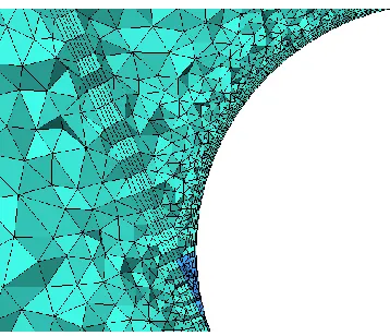
Figure 4-6 demonstrates the cross section of tiny elements around the roll surface compared

to the other cells far away from the roll. A closer view of the grid is depicted in Figure

4-7. It is obvious that due to the costly calculation time, creating tiny elements in the whole

domain is not necessary, especially when the study concentration is known.

(36)

Figure 4- 7: Close-up view of the mesh grid close to the sink roll

Prism layers are also used to create a mesh with higher aspect ratio at the wedge area shown

in Figure 4-8. Creating smaller surface elements or using prism layers could not totally

remove the skewed elements within the area of interest. Therefore, in an innovative

approach all the four areas consist of skewed elements are separated and referred to as

patch areas. As displayed in Figure 4-9, these areas are filled with tiny fluid elements to

reduce the mesh skewedness.

(37)

Figure 4- 9: Improvement of volume elements at the wedge area

4.5 Simulation Conditions

The dynamic behavior of the fluid inside the bath is simulated using realizable 𝑘-𝜀 method

in Ansys FLUENT. This is due to its reliability as a RANS model for free stream turbulence

modeling and inexpensive computational cost [36]. The fluid property in a fixed

temperature condition has been set for the simulation [37]. The simulation has been

continued with the convergence rate of 1.0E-5 for the continuity, velocity components, 𝑘

and 𝜀 .Constant bath fluid properties are used for the calculations at 460℃; density ρ=6600

kg/m3 and viscosity μ=0.004 Pa.s. [38].

In this study standard wall function (SWF) has been defined for law of the wall in the

modeling. Therefore, 𝑌+_{parameter is checked to be in the valid regime which is}

30<𝑌+<300. 𝑌+ is a non-dimensional wall distance for a wall-bounded flow.

𝑌+ ₌𝑌 𝑢∗

𝑣 (4-1)

In this equation, 𝑢∗ is the friction velocity at the nearest wall, 𝑌 is the distance to the nearest

wall and 𝑣 is the local kinematic viscosity of the fluid. 𝑌+_{is often referred to simply as y}

(38)

Table 4- 2: Parameters used for the CFD study of liquid phase

Material Liquid Zinc Fluid density (kg/m3₎ ₆₆₀₀

Fluid viscosity (kg/ms) 0.004 Fluid turbulence model 𝑘-𝜀

Discretization method Second order

Time Steady-state

Convergence rate 1e-5 Cell type Tetrahedral Number of cells 1.5, 2.5 and 5M Processing style 8 parallel processes

4.6 Bath fluid flow results

The following results are obtained from simulation of fluid flow in the galvanizing bath.

Velocity contours at the middle of the bath are shown in Figure 4-10. Fluid flow behaviour

within the bath at selected cross sections are depicted in Figure 4-11 and 12.

(39)

Figure 4- 11: Displaying of the cut-planes in the bath

Figure 4- 12: Top view of the defined cut-planes in the bath

Figure 4-13 displays the velocity vectors at the mid plane of the bath (Z=0). The rotation

of the rolls and submerging the strip down to the bath create a vortex at the top of the sink

roll, which conforms to the literature. X=0m

Z=0m

(40)

Figure 4- 13: Velocity vectors at the middle of the bath

According to the bath water model experiments performed by Gagné et al. [11] and

numerical simulations conducted by Ilinca et al.[16], the fluid flow pattern structure shows

a good agreement.

Ouellet’s [14] numerical study, which was validated by PIV experimental method

discussed in chapter 3, also conforms to the obtained simulations results from the 3-D bath

model in the vortex formed on top of the sink roll at the center line of the galvanizing bath.

Figure 4-14 shows the velocity vectors at the X-Z plane, where it cuts the sink roll from the

center. The flow structure is symmetric as expected. It displays two vortices on each side

of the roll near the steel strip. Velocity contours at this plane also depicted in Figure 4-15,

which indicate the velocity gradient at the strip-roll area. A better view of the velocity

vectors is demonstrated in Figure 4-16. It shows how fluid flow inside the wedge area

(41)

Figure 4- 14: Velocity vectors at the X-Z cut-plane (y=0)

Figure 4- 15: Velocity contours at the X-Z cut-plane (y=0)

(42)

Figure 4- 17: Velocity vectors at the Y-Z cut-plane

Figure 4-17 displays the velocity field at the wedge area. It can be seen that the zinc fluid

becomes trapped by the moving converging surfaces and then is pushed out into the open

area along the roll in Y-Z plane where the strip ends.

The reason that the fluid is being pushed out toward both ends is that there are two

converging surfaces moving in the same direction. According to the no-slip condition that

was defined for walls, the fluid on each wall will have the same velocity as the walls. Since

the moving strip and roll converge, the fluid will have different flow patterns as it travels

away from the roll symmetry line. The zinc fluid is then pushed out from the roll center to

strip edges, where it can flow freely. (Note: the width of the strip is less than the sink roll.)

The velocity vectors on the steel strip are shown in Figure 4-18. It displays the direction

changing of the velocity vectors where it reaches the strip edge. Figure 4-19, the fluid flow

is depicted in a 3-D view of the roll. Velocity vectors in Figure 4-18 depict how the fluid

flows on the moving strip. Figure 4-19 shows that the flow with higher velocity is located

(43)

Figure 4- 18: Velocity vectors on the strip

Figure 4- 19: Fluid flow direction at the wedge area

4.7 Particle-surface study

Based on the reports form industries, suspended dross particles in hot-dip galvanizing bath,

can interact with the surface of the moving roll and eventually accumulate on it. To

understand how dross particle interact with the hardware components, it is important to

elaborate on tracking of dross particles in an industrial galvanizing bath.

This study examines particle-surface interactions near the sink roll surface in a galvanizing

(44)

liquid-solid models. Particle trajectories has been studied for better understanding of our project

objective which is the particle build-up mechanism on the roll surface. It is based on the

hypothesis that particles agglomerate at the same location as they collide with the roll

surface in the bath. The advantages and drawbacks of different multiphase models will be

briefly described.

4.8 Previous studies

Numerical simulations can help us in better understanding of the fluid flow and in

improving the knowledge of dross particle tracking in a galvanizing bath. Some methods

have been proposed to remove the agglomerated bottom dross from the bath [39].

Fundamental fluid flow studies in a galvanizing bath have been carried out by different

researchers [40].

It is evident from the previous study that the 3-D fluid flow in the bath becomes

concentrated near the sink roll, where it meets the strip. This is significant because it

addresses the dross particle interaction locations on the roll, where the particles most likely

agglomerate on the roll surface.

Tracking of massless particles is studied in an experimental work performed by Willis et

al. [17,18]. They observed number of particles settle at the bottom of the bath increased

with particle size. Pare et al. [19] tracked particles with different densities at different

locations: starting from center of the bath and back of strip. They found that the particle

path lines depend on their densities and the initial position they are released. Kurobe et al.

[41] used polystyrene particles and NaCl aqueous solutions to model dross and bath liquid,

results showed that the particles become concentrated on top of the moving roll, where the

strip enters and exits. In another study, the behavior of dross particles are examined by

Gagné et al. [11] in a half scale galvanizing bath model. They observed the trajectories of

polymeric particles with a video camera to determine the fluid flow pattern in the bath.

In some numerical studies, different multiphase models have been used to simulate the

particle trajectories in several studies. In a study by Ibsen et al. [42], different multiphase

(45)

phase model is in a better agreement with the experimental observations, compared to the

simulation results of continuum-continuum approach. Chu et al. [43] reported a detailed

comparison of Eulerian-Eulerian model with discrete particle model for a fluidized bed.

Rosato et al. [44] proposed a method for particles tracking such a way that particles are

displaced step-wise. Then the fluid effect is studied through the computational domain.

4.9 Mathematical Models

There are two popular modeling approaches used for multiphase (liquid-solid) flow

problems. They include macroscopic continuum-continuum approach introduced by

Eulerian-Eulerian model which focuses on the behavior of bulk fluid flow and microscopic

continuum–discrete approach defined by Eulerian-Lagrangian model [45].

4.9.1 Eulerian-Eulerian Approach

This approach treats both solid and liquid phases as a continuum. The method is relatively

fast, since it requires less numerical computations compared to continuum-discrete

approach [45]. In this approach, general behavior of the fluid phase is detailed and the

detail information of the solid phase is not considered .Consequently, dilute multiphase

flows consisting of small numbers of particles cannot be modeled using this approach.

According to the nature of the current study, the Eulerian-Lagrangian approach is of main

interest and will be discussed in the following sections.

4.9.2

E

ulerian-Lagrangian Approach

In the continuum-discrete approach, the fluid behavior is determined by solving the

Navier-Stokes equations, whereas the solid particle motion is defined using Newton’s law of

motion for individual particles with their coupling of Newton’s third law of motion. This

approach, can provide detailed information about the particles trajectories and the transient

particle- particle and particle-fluid forces [45,46]. Many such methods have been

developed over the past decades that can be divided into two models: Discrete Phase Model

(46)

The main advantage of DPM model is the fast computational time, since it does not

consider the collision effect that might be significant in some multiphase flows and mixing

processes.

In the present work, the details of DPM and DEM multiphase models are briefly elaborated.

For particle modeling, coupling of liquid with the particles is presented for three different

cases: DPM for massless particles, DPM for particles with mass and DEM for particles

with mass.

To simulate the particle trajectories in a galvanizing bath, there is no need to develop new

codes for these complex models, since they are validated and available in CFD modeling

software such as Ansys FLUENT, EDEM or OpenFOAM. Developing complex

multi-scale geometry with turbulent multiphase flow is very time consuming. Thus, Ansys

FLUENT has been employed as a platform. This model is extended using a DEM solver,

incorporating a User Defined Function code to evaluate the particle-surface interactions

and quantify the presence of particles in the extreme vicinities of the moving roll.

4.10 CFD Modeling

The liquid and fluid phase modeling is described in the following sections.

4.10.1 Liquid phase modeling

The continuum fluid phase in the presence of a secondary particulate phase is solved for

each computational cell from the continuity and modified Navier-Stokes equations as

shown in equations 4-1 and 4-2. [43].

∂(𝜀𝑓)

𝜕𝑡 + ∇. (𝜀𝑓𝑢𝑓) = 0 (4-1)

𝜕(𝜌𝑓𝜀𝑓𝑢𝑓)

𝜕𝑡 + 𝛻. (𝜌𝑓𝜀𝑓𝑢𝑓𝑢𝑓) = −𝜀𝑓𝛻𝑝−𝐹𝑓 𝑝

+ 𝜀_𝑓𝛻. 𝜏 + 𝜌_𝑓𝜀_𝑓𝑔 (4-2)

Where 𝜀𝑓 is the volume fraction occupied by the fluid, 𝜌𝑓 is the fluid density, 𝒖𝑓 is the

(47)

force which represents the particle drag force, the pressure gradient force, and the viscous

force.

4.10.2 Particulate Modeling

In this work, two different multiphase models including Discrete Phase Model

(CFD-DPM) and Discrete Element Method (CFD-DEM) are employed to study particle motion

near the moving surfaces.

It is clear that due to the fluid and particle-particle interactions and particle-particle

interactions, simulation of the hydrodynamic of liquid–solid flow is quite complex.

However, many efforts with the development of advanced computational techniques and

high speed processors have been made, in order to study the complex multiphase flows

including high density mesh grid and steady/unsteady discrete phase motion. These models

are mainly achieved by coupling the discrete phase model (DPM) for solid phase with

computational fluid dynamics (CFD) for fluid phase known as CFD-DPM. In this model

the detailed dynamic behavior for both phases and forces of particles are still unknown

[45]. Therefore the new approach, known as CFD-DEM approach, is proposed to

understand the physics of liquid–solid flows. Both DPM and DEM models are

continuum-discrete approaches which use Lagrangian particle tracking. This work studies the two

different multiphase models CFD-DPM and CFD-DEM to understand particle motion near

the moving surfaces.

4.11 Discrete Phase Modeling

Lagrangian particle tracking is based on a translational force balance that is defined for an

individual solid particle. Each particle represents a parcel of particles which is subject to

gravity, drag force, buoyancy. DPM capabilities allow us to simulate the particle motion

without considering the particle-particle collision effects. Therefore, if the particle-particle

or particle-wall collisions are insignificant, this method can be employed to simulate the

particle behavior in the multiphase flow. Because of the assumptions and simplifications,

(48)

4.12 Discrete Element Modeling

DEM is a time-driven particle modeling approach which first proposed by Cundall and

Strack [48]. The applications of the DEM approach vary depending on the flow geometry,

the accounting of forces acting on each particle and in the method of coupling between the

discrete and liquid phase. Coupling of CFD with DEM can provide detailed information

about particles trajectories by solving system of N-Lagrangian equation of motion for each

particle as given in equation 4-3.

𝑀𝑑𝑣

𝑑𝑡 = 𝐹𝑡𝑜𝑡𝑎𝑙 (4-3)

M is a matrix of particle mass, 𝑣 is a y vector of the interacting particles and 𝐹_{𝑡𝑜𝑡𝑎𝑙}is a sum

of the forces such as hydrodynamic (gravitational, drag and buoyant) terms and

non-hydrodynamic (cohesive, colloidal and electrostatic and van-der-Waals) [49]. The main

disadvantage of DEM approach is its high computational time to solve the full matrix for

the transient solutions related to each particle.

After computing the total force acting on each particle, Newton’s equation of motion can

be integrated numerically to determine the particle velocity and integrating again, the

position of all particles at the current time will be known as shown in equations 4 and

4-5 [44-5]. 𝑚𝑑𝑣𝑖 𝑑𝑡 = ∑ (𝐹𝑐,𝑖𝑗 𝑝 + 𝐹𝑔,𝑖+ 𝑁 𝑗 𝐹𝑓,𝑖 𝑝

) (4-4)

𝐼_𝑖𝑑𝜔𝑖

𝑑𝑡 = ∑ (𝑇𝑖,𝑗 𝑝 𝑁

𝑗 ) (4-5)

Where 𝑚𝑖, 𝐼𝑖, 𝑣𝑖 and 𝜔𝑖 are the mass, moment of inertia, translational and rotational

velocity of particle i. The forces are: gravitational force 𝐹𝑔,𝑖, contact forces 𝐹𝑐,𝑖𝑗 𝑝

, 𝐹_𝑓,𝑖𝑝 is the

particle-fluid interaction force and 𝑇_𝑖,𝑗𝑝 is the torque between particle 𝑖 and 𝑗. Due to the

nature of the present work and relatively large particles, non-direct contact forces such as

(49)

4.13 Collision Modeling

Collision force can affect the interaction between the particles and between particles and

walls. The collision force is calculated based on a soft-sphere method using DEM which

allows the particle to overlap, during collisions normally less than 0.5% of the particle

diameter [50]. This overlap is used to calculate elastic, plastic and frictional forces between

particles [48]. Very small time step are required to achieve precise information at each

collisions which will lead to high computational time. Many efforts have been carried out

to reduce the computational time by simplifying these models. However, the most common

linear model is the linear spring–dashpot model which was proposed by Cundall and Strack

[48]. In this collision model, spring represents the elastic deformation while dashpot

accounts for the viscous dissipation.

Particle collisions are modeled using Hertzian contact model [51]. The collision force has

a normal and a tangential component in which the normal force acts in a direction

connecting the center of particles and is defined as:

(4-5)

A linear normal damping force is also assumed in this work [36]. The linear spring-dashpot

model is used for the tangential component of collision force.

(4-6)

K_𝑡 and 𝐶_𝑡 are the tangential spring and dashpot coefficients, 𝜇_𝑠is the static coefficient of

friction. 𝛿_𝑖 is the overlap between particles in contact in normal (𝑛) and tangential (𝑡)

directions. Tsuji et al. [52] assumed that tangential dissipation coefficient is in the same

order of magnitude as the normal damping coefficient Ct = Cn. In this work the tangential

damping coefficient is assumed similar to the normal one.

4.14 Coupling between the phases and time step size

To accounting for interaction effects, four-way coupling between the two phases is required

which is computationally expensive and sometimes risky to converge. Fluid affects the 

n n

n c

k

F  3/2 

|) | ,

min( t t t t s N

t k c F

F   

(50)

particles and particles affect the fluid in addition to the effects of particle-particle collisions

[48]. CFD-DEM runs the CFD and DEM solvers either simultaneously or in consecutively

with the interval of usually 50-100 time-steps. Time-step for DEM needs to be extremely

small to capture the inter-particle collisions than the time-step for CFD. Therefore, DEM

solver has to run several time steps before transferring the solid particle data to CFD solver.

The coupling is numerically achieved such a way that at each time step, DEM will provide

the solid phase information such as position and velocity for each particle. Solver uses the

particle data and the volume fraction in each computational cell to update the fluid flow

field by calculating the momentum exchange terms between the phases. Incorporation of

the resulting forces into DEM will result in the particle motion for the next time step. Then

the particle affects the fluid phase from the particles, so that Newton's third law of motion

is satisfied [36].

4.15 Simulation Conditions

For the liquid phase, the dynamic behavior of the molten zinc inside the bath is already

simulated. Realizable 𝑘-𝜀 method is used due to its reliability as a RANS model for free

stream turbulence modeling and for being relatively computationally inexpensive.

The discrete element method is used to track particles with different concentration near the

sink roll surface. Ansys FLUENT has a number of different DEM collision models

available [36]. In this work, linear Hook law model, which is a combination of a contact

force and a damping force was selected to calculate the normal and tangential force for

both collisions. The contact forces due to particle-particle or particle-wall collisions are

evaluated in terms of the normal and tangential coefficients of restitution Bottom dross

particles are assumed as identical spheres with constant radius (100 microns) and density

(7230 kg/m3_{) [5]. Table 4-3 shows the parameters used in this simulation for the liquid and}

(51)

Table 4- 3: Parameters used for the DPM and DEM studies of solid phase

Parameter DPM DEM

Particle Shape (𝑚) Sphere Sphere

Particle Size (𝜇𝑚) 100 100

Particle Density (𝑘𝑔/𝑚^3) 7230 7230 Number of Particles 1, 200 and 1000 200 and 1000

Particle Type Massless/ Inert Inert

Injection Location In front of the strip and on top of the roll

In front of the strip and on top of the roll Particle-particle

Collision

Particle-particle Collison is Neglected

Overlap- Soft-sphere

Dynamic Friction Coefficient 0.25 m 0.25 m Interaction with the Fluid Phase 1-way 4-way

Application Dilute particle flows Dilute/Dense flows Normal Coefficients of

Restitution

- 0.9

Coefficient of Dynamic Friction - 0.3 Solid Phase Time Step (s) - 1e-5

4.16 Particle-surface study results

As shown previously, it is evident that there is an insignificant influence of the moving hardware on fluid flow in the bulk of the zinc bath. However, further studies of the V-section showed the fluid tendency to move from the center of the roll toward its both ends.

(52)

Figure 4- 20: Locations for particle injections in the galvanizing bath

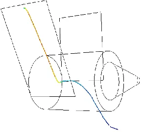
Figures 4-21 and 4-22 display the particle trajectories obtained from DEM simulation for injection 1 and injection 2. It is observed that the released particles are dragged to the bath due to the strip high velocity motion. It can be concluded that particles with mass released from different locations follow the bulk fluid flow inside the bath. It was discovered that dross particles starting from the snout region remain in the V-section and move toward the sink roll top surface. This is due to the small difference in densities (9%) of the bath fluid and dross particle. The circulating motion of fluid in this region moves the dross particles toward the top surface of sink roll.

Injection 1

(53)

Figure 4- 21: Injection 1- From snout region in front of the strip

Figure 4- 22: Injection 2-From top of the sink roll

(54)

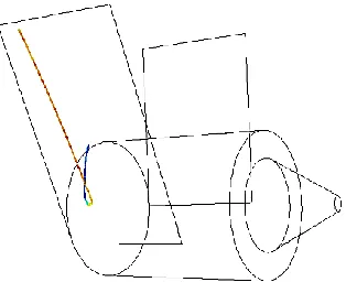
Figure 4- 23: DPM Particle trajectory for a particle close to the middle of the roll

Figure 4- 24: DPM Particle trajectory for a particle closer to strip edge

Figure 4- 25: DPM Particle trajectory for single particle released from strip edge

Improving Galvanizing Bath Hardware

Scholarship@Western

Scholarship@Western

Improving Galvanizing Bath Hardware

Improving Galvanizing Bath Hardware

Abstract

Keywords

Acknowledgments

Table of Contents

List of Tables

List of Figures

Nomenclature

Chapter 1

1.1

Introduction

1.2

Galvanizing Process Description

1.3

Dross Particle

1.4

Primary sources of dross formation

1.5

Goal of this project

1.6

Outline of thesis

Chapter 2

2

Literature Review

2.1

Previous Studies

2.2

Summary

Chapter 3

3

Numerical Setup

3.1

Multiphase flow

3.1.1

Eulerian- Lagrangian approach

3.2

Governing equations

3.2.1

Particle Equation of motion

3.3

Particle Transport Mechanisms

Chapter 4

4

3-D fluid flow study in the bath

4.1

Fluid flow studies

4.2

Computational Domain

4.3

Numerical Procedure

4.4

Mesh Grid Generation

4.5

Simulation Conditions

4.6

Bath fluid flow results

4.7

Particle-surface study

4.8

Previous studies

4.9

Mathematical Models

4.9.1

Eulerian-Eulerian Approach

4.9.2

ulerian-Lagrangian Approach

4.10

CFD Modeling

4.10.1 Liquid phase modeling

4.10.2 Particulate Modeling

4.11

Discrete Phase Modeling

4.12

Discrete Element Modeling

4.13

Collision Modeling