Adaptive Non-Local Means using Weight Thresholding

(1)

Scholarship@Western

Electronic Thesis and Dissertation Repository

12-9-2015 12:00 AM

Adaptive Non-Local Means using Weight Thresholding

Asif Khan

The University of Western Ontario

Supervisor

Dr. Mahmoud R. El-Sakka

The University of Western Ontario

Graduate Program in Computer Science

A thesis submitted in partial fulfillment of the requirements for the degree in Master of Science © Asif Khan 2015

Follow this and additional works at: https://ir.lib.uwo.ca/etd

Part of the Computer Sciences Commons

Recommended Citation Recommended Citation

Khan, Asif, "Adaptive Non-Local Means using Weight Thresholding" (2015). Electronic Thesis and Dissertation Repository. 3369.

https://ir.lib.uwo.ca/etd/3369

This Dissertation/Thesis is brought to you for free and open access by Scholarship@Western. It has been accepted for inclusion in Electronic Thesis and Dissertation Repository by an authorized administrator of

(2)

(Thesis format: Monograph)

by

Asif Khan

Graduate Program in Department of Computer Science

A thesis submitted in partial fulfillment

of the requirements for the degree of

Masters of Science

The School of Graduate and Postdoctoral Studies

The University of Western Ontario

London, Ontario, Canada

c

(3)

Non-local means (NLM) is a popular image denoising scheme for reducing additive

Gaus-sian noise. It uses a patch-based approach to find similar regions within a search neighborhood

and estimate the denoised pixel based on the weighted average of all the pixels in the

neigh-borhood. All the pixels are considered for averaging, irrespective of the value of their weights.

This thesis proposes an improved variant of the original NLM scheme, calledWeight

Thresh-olded Non-Local Means(WTNLM), by thresholding the weights of the pixels within the search

neighborhood, where thethresholded weightsare used in the averaging step. The key

parame-ters of the WTNLM are defined using learning-based models. In addition, the proposed method

is used as a two-step approach for image denoising. At the first step, WTNLM is applied to

generate a basic estimate of the denoised image. The second step applies WTNLM once more

but with different smoothing strength. Experiments show that the denoising performance of

the proposed method is better than that of the original NLM scheme, and its variants. It also

outperforms the state-of-the-art image denoising scheme, BM3D, but only at low noise levels

(σ≤ 80).

Keywords: Image denoising, Additive Gaussian Noise, local Means, Two-stage

Non-local means, Spatial Domain Denoising

(4)

I am expressing my heartiest gratitude to the Almighty to give me the ability to complete my

thesis successfully. I would like to thank my thesis supervisor Dr. Mahmoud R. El-Sakka for

his noteworthy and valuable direction, guidance, motivation and encouragement in the way of

my progress. It was an absolute honor and privilege to work with such a modest and wise

person like him. Moreover, I am also thankful to all of my professors from the University of

Western Ontario for building my background to complete this task.

I am also grateful to my family for their continuous support and guidance.

(5)

Abstract ii

Acknowledgments iii

List of Figures vii

List of Tables ix

1 Introduction 1

1.1 Motivation . . . 2

1.2 Thesis Contribution . . . 2

1.3 Thesis Outline . . . 3

2 Background 4 2.1 Image Noise . . . 4

2.1.1 Additive Noise . . . 4

White Gaussian Noise . . . 5

Estimating additive white Gaussian noise . . . 6

2.1.2 Multiplicative Noise . . . 7

2.1.3 Salt & Pepper Noise . . . 7

2.2 Image Denoising . . . 7

2.2.1 Spatial Domain Approach . . . 8

2.2.2 Frequency Domain Approach . . . 8

(6)

2.3.1 Mean Filter . . . 9

2.3.2 Median Filter . . . 9

2.3.3 Gaussian smoothing . . . 10

2.3.4 Anisotropic Diffusion . . . 10

2.3.5 2-D Adaptive Wiener Filter . . . 11

2.4 Frequency Domain Methods . . . 12

2.4.1 Low-Pass Filter . . . 12

2.4.2 Wiener Filter . . . 13

2.4.3 BM3D . . . 14

2.4.4 BM3D Extensions . . . 16

BM3D Denoising using Shape-Adaptive Principal Component Analysis 16 BM3D Denoising using SSIM Optimized Wiener Filter . . . 16

2.5 Non-Local Means . . . 17

2.6 Non-Local Means Variants . . . 18

2.6.1 Principal Components of Non-Local Means . . . 18

2.6.2 Improved Non-Local Means based on dimensionality reduction . . . 19

2.6.3 SSIM-based Non-Local Means . . . 20

2.6.4 Iterative Non-Local Means . . . 20

2.6.5 Non-Local Euclidean Median . . . 21

2.6.6 Two-stage Non-Local Means with adaptive smoothing parameters . . . 21

2.7 Non-Local Means Applications . . . 22

3 Methodology 23 3.1 Adaptive Non-Local Means using Weight Thresholding . . . 23

3.2 Parameter Selection . . . 25

3.2.1 Cut-offWeight for Thresholding . . . 26

(7)

Exponential Model . . . 28

3.2.2 Patch Size and Search Window Size . . . 28

3.2.3 The two-step approach . . . 37

3.3 Summary of the selected parameters . . . 39

4 Experimental Results and Analysis 40 4.1 Image set . . . 40

4.2 Noise Generation . . . 40

4.3 Performance Measure . . . 42

4.3.1 Peak Signal to Noise Ratio (PSNR) . . . 43

4.3.2 Mean Structural Similarity (MSSIM) . . . 43

4.4 Results and Analysis . . . 45

4.4.1 Performance evaluation using PSNR . . . 45

4.4.2 Performance evaluation using MSSIM . . . 48

4.4.3 Visual Comparison . . . 51

4.4.4 Intensity Profile . . . 62

4.5 Summary . . . 66

5 Conclusion and Future Work 67 5.1 Conclusion . . . 67

5.2 Future Work . . . 68

Bibliography 69

Curriculum Vitae 74

(8)

2.1 Probability density function of Gaussian random variable . . . 5

2.2 Image affected with additive white Gaussian noise (a) Noise-free image. (b) Image affected with Gaussian noise (σ= 40) . . . 6

2.3 BM3D Block Diagram . . . 14

3.1 Training image set (a) Lena. (b) Barbara (c) Peppers (d) Baboon (e) Boats . . . 26

3.2 Bar chart of PSNR for different linear models (changing the coefficienta) . . . 27

3.3 Bar chart of PSNR comparison between different exponential models (chang-ing coefficienta) . . . 29

3.4 Bar chart of PSNR comparison between different search window size . . . 30

3.5 PSNR comparison between different patch sizes (a) Noise,σ5 - 50 (b) Noise, σ55-100 . . . 33

3.6 Plot of optimal search window for various noise levels . . . 35

3.7 Curve fitting using a linear model . . . 35

3.8 Curve fitting using a quadratic model . . . 36

3.9 Curve fitting using a exponential model . . . 36

3.10 Bar chart of PSNR comparison of proposed method for multiple steps . . . 38

4.1 Kodak Image Set (Grayscale) . . . 41

4.2 Example of Gaussian noise (σ=40) added to a noise-free image . . . 42

4.3 Bar chart of PSNR comparison of proposed and existing methods . . . 47

4.4 Bar chart of MSSIM comparison of proposed and existing methods . . . 50

(9)

4.6 Visual Comparison forσ=40 . . . 53

4.10 Visual Comparison (Zoom) forσ=20 . . . 57

4.15 Row number 100 ofGirlimage used for generating intensity profile. Scan line shown as a red line. . . 63

4.16 Intensity Profile Comparison of the Girl image at scan line 100 (σ =40) . . . . 64

4.17 Intensity Profile Comparison of the Girl image at scan line 100 (σ =80) . . . . 65

(10)

3.1 PSNR Comparison of linear models for different coefficienta . . . 27

3.2 PSNR Comparison between exponential models for different coefficienta . . . 29

3.3 PSNR Comparison by changing the search window size . . . 30

3.4 PSNR Comparison for fine tuning the search window size . . . 31

3.5 PSNR Comparison by changing the patch size . . . 32

3.6 PSNR Comparison by fixing patch size=9×9 and changing search window size 34

3.7 PSNR comparison of proposed method for multiple steps for various noise levels 38

4.1 PSNR comparison of theGirl image among the proposed method, the NLM

method, variants of NLM and BM3D denoising scheme for various noise levels 46

4.2 PSNR comparison of the proposed method, the NLM method, variants of NLM

and BM3D denoising scheme for various noise levels . . . 46

4.3 Standard deviation of PSNR values of proposed method and existing methods

for different noise levels . . . 47

4.4 MSSIM comparison of theGirlimage among the proposed method, the NLM

method, variants of NLM and BM3D denoising scheme for various noise levels 49

4.5 MSSIM comparison of the proposed method, the NLM method, variants of

NLM and BM3D denoising scheme for various noise levels . . . 49

4.6 Standard deviation of MSSIM values of proposed method and existing methods

for different noise levels . . . 50

(11)

image, the NLM method, variants of NLM and BM3D denoising scheme for

noiseσ= 40 . . . 63

4.8 Pearson correlation coefficient comparison of the proposed method, the noisy

image, the NLM method, variants of NLM and BM3D denoising scheme for

noiseσ= 80 . . . 63

(12)

Introduction

A digital image is made of finite number of elements, called pixels and can be defined as a

two dimensional function. For grayscale images, the pixel intensity, also referred to as

gray-scale value, takes on values between 0 and 255, where 0 represents the darkest pixel and 255

represents the brightest pixel.

The pixels of a digital image can be contaminated with noise which results in random

variation of brightness in the image. The noise is introduced during the image acquisition

phase due to image sensors, in low light environment, or during transmission. Image denoising

is the process of estimating the original image from a given noisy image and is one of the most

fundamental problems in image processing. For an imaging application, working with noisy

images can significantly affect the performance and reliability of the overall system. Image

denoising is used as a pre-processing step in imaging applications to reduce the amount of

noise and a major challenge is to reduce as much noise as possible while still keeping most of

the visual information, such as edges and textures.

(13)

1.1 Motivation

Earlier approaches to image denoising consisted of methods which attempt to estimate the

denoised value of a pixel based on the information in a local area around each pixel. While such

methods have been successful, to some extent, the resulting denoised images are often blurry.

Buades et al. proposed the Non-Local Means (NLM) denoising scheme [3][4], using a

non-local patch based concept. It attempts to identify self-similarities in a noisy image and calculate

a weighted average of similar pixels in order to estimate a denoised image. Although many

variants has been proposed after the original non-local means scheme, there are still room for

improvements. The underlying nature of non-local means using all pixels in a defined search

area tends to deviate the estimated denoised pixel value from the true noise-free intensity. In

addition, the key parameters of the original NLM are kept fixed, irrespective of the amount

of noise in the noisy image. One of our focus is to propose a variant of the non-local means

scheme for better denoising performance. Another focus is to empirically define a set of models

for determining the value of the key parameters, based on the noise level of a given image.

1.2 Thesis Contribution

The original non-local means denoising scheme considers all the pixels, defined within a search

area, for calculating the weighted average of the denoised image. This includes all the pixels

which are not similar to the reference pixel being denoised. Even with low weights, the pixels

which are not similar to the reference pixel being denoised will move the estimated denoised

intensity value from the true intensity. In our proposed method, we have thresholded the pixel

weights against a cut-offweight to use only a subset of the available pixels for calculating the

weighted average. In the original non-local means and its variants, the search window size

and patch size are fixed, irrespective of the level of noise. In our proposed method, we have

(14)

level. The models are determined using a learning based approach. We have also applied our

proposed method as a two-step process, where the basic denoised output of the first step is

further processed to remove remaining noise artifacts, especially at high noise levels.

1.3 Thesis Outline

The thesis is divided into five chapters. The current introductory chapter isChapter 1, where

we have outlined the objectives and thesis contributions. In Chapter 2, we discussed the

background of image denoising in details. InChapter 3, we introduced our proposed method

in details and explained the parameters selection procedure that we adopted in our proposed

method. In Chapter 4, we presented the experimental results of our proposed method and

compared them to that of the existing image denoising schemes. Finally, in Chapter 5 we

(15)

Background

2.1 Image Noise

Noise is a random signal which corrupts the original signal by adding unwanted information

to the signal. In a digital image, noise is a random variation of brightness. It is usually

pro-duced during the image acquisition phase, caused by the sensors of digital cameras or scanners.

Modern digital cameras have come a long way in using high quality sensors which have

sig-nificantly reduced the presence of noise during image acquisition yet, noise still can affect the

quality of an image, especially in low light conditions.

Digital noise types include: Additive noise,Salt and Pepper NoiseandMultiplicative noise.

2.1.1 Additive Noise

Additive noise gets added with the image signal. An image affected by additive noise can be

modeled using:

v(i)= u(i)+n(i), (2.1)

wherev(i) is the observed gray value at pixeli,u(i) is the noise-free gray value andn(i) is the

amount of noise at pixeli.

(16)

White Gaussian Noise

White noise is a random signal with a constant power spectral density [9]. Gaussian noise is a

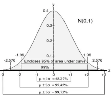
statistical noise which follows the Gaussian distribution. The probability density function of a

Gaussian random variable,z, is modeled as shown:

p(z)= √1

2πσe

−(z−µ)2

2σ2 , (2.2)

wherezrepresents gray level,µis the mean,σis the standard deviation of the distribution, also

referred to as the noise density of the Gaussian noise signal, and σ2 is the variance. Figure

2.1 shows the probability density distribution of a Gaussian model. Almost all the area under

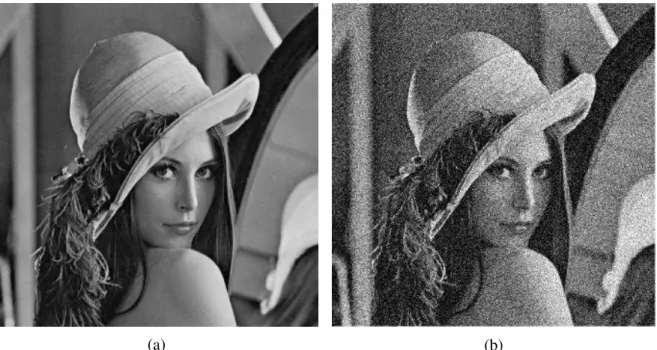
the curve lies betweenµ±3σ. Figure 2.2 shows an example of an image which is affected by

additive white Gaussian noise withσ=40.

(17)

(a) (b)

Figure 2.2: Image affected with additive white Gaussian noise (a) Noise-free image. (b) Image affected with Gaussian noise (σ=40)

Estimating additive white Gaussian noise

For optimal denoising of digital images affected with additive Gaussian noise, most methods

require some knowledge of the noise density,σ. Although the exact noise density may not be

possible to be known beforehand, a good estimation can be calculated. One of the methods

for estimating noise is the local variance method [1]. For estimating the noise density, a given

noisy image is divided in small sub-blocks. The gray value variance is calculated for each

sub-block and the variance of all the sub-blocks are averaged to estimate the noise variance

of the Gaussian noise. The noise density is the square root of the average variance. The size

of the sub-images used for calculating the value ofσ should ideally be the smallest possible

(18)

2.1.2 Multiplicative Noise

Multiplicative noise is a random signal which gets multiplied to the original signal.

Multiplica-tive noise can be modeled as shown:

v(i)= u(i)×n(i), (2.3)

wherev(i) is the observed gray value for pixeli,u(i) is the noise-free value andn(i) is the noise

at pixeli. Most common form of multiplicative noise isspeckle noise. Common methods for

removing speckle noise include Lee filter [18] and Frost filter [8].

2.1.3 Salt & Pepper Noise

Salt and Pepper noise is a form of impulse noise where the gray level of the affected pixels are

either changed to the maximum possible intensity level (255 in case of 8-bit grayscale images)

or to the minimum possible intensity value (0) . The noise appears as white and black pixels

(or dots) in the image and the noise density,d, of the salt-and-pepper noise is determined by

the number of pixels affected by the noise. It affects approximately d× N × M pixels in an

image, where d satisfies the condition 0 ≤ d ≤ 1 and N × M is the number of pixels in the

image.

2.2 Image Denoising

Most imaging system have an image acquisition phase and the performance of the overall

system depends on the quality of the image. The level of noise in the image plays a critical

role in the outcome of the system and it is desirable to have as much reduced noise as possible

during the image acquisition phase. Any noise added during this phase is first denoised before

(19)

while preserving the texture and edges of the image. A scheme which is able to reduce most

of the noise but completely blurs the entire image to a point where minimal visual information

can be extracted is not ideal. Similarly a denoising method which preserves a lot of the texture

in the image but fails to remove the noise to a satisfactory level is not an effective method as

well.

The image denoising methods can be classified primarily into two groups, based on the

approach they use for reducing noise effect:spatial domain approachesandfrequency domain

approaches

2.2.1 Spatial Domain Approach

The term spatial domain refers to the image plane itself [9]. In this domain, the raw observed

gray values of a noisy image are manipulated for estimating the denoised image. It takes

ad-vantage of the notion that pixels in a small local neighborhood are correlated. Spatial domain

approaches can be denoted by the expression g(x,y) = T[f(x,y)], where f(x,y) is an input

image,g(x,y) is the output, or, processed image andT is some operator defined over a

neigh-borhood of (x,y).

The neighborhood around an image pixel at position (x,y) is defined as a rectangular or

square sub-image centered at position (x,y). The size of the window is selected based on the

operation performed over the selected sub-image. The operatorT is usually applied over

sub-images centered on each pixels in the given image. The resulting processed image is considered

as the denoised image.

2.2.2 Frequency Domain Approach

In frequency domain approaches, the image is transformed to the frequency domain using, for

example, Fourier transform or wavelet transform. The frequency domain separates smooth

(20)

fre-quencies, thus making it easier to target and enhance certain regions in an image.

2.3 Spatial Domain Methods

This section covers some of the common spatial domain denoising methods. The spatial

do-main methods tries to estimate the denoised images based on the raw intensity value of image

pixels.

2.3.1 Mean Filter

The mean filter is a method of smoothing the image to reduce the noise in the image. The

mean filter operates by replacing the pixels in the image with the mean/average of the pixels

in a local neighborhood, including itself [9]. This helps reduce the pixel intensities which are

unrepresentative of its neighborhood. Mean filter is a convolution method and is based on a

kernel. The size of the kernel determines the degree of smoothing around each pixel. The

weights assigned to each position in the kernel can either be equal or can be weighted based

on the proximity to the center of the kernel. For example, if weights are assigned following

a Gaussian model then the pixels closer to the center will have more weights than the pixels

further from the center and the sum of the weights equals 1.

2.3.2 Median Filter

The median filter looks to remove noise by estimating the noise-free gray value based on the

median of the intensities of the pixels around the local neighborhood of a reference pixel [9]. A

N×Nwindow is centered around each pixels in the image and the pixel intensity of the center

is replaced by the median gray value of the pixels within the window. Compared to the mean

filter, median filter is more robust to the presence of outliers within the local window. Unlike

(21)

ignores outliers. The median filter is also used for denoising salt-and-pepper noise.

2.3.3 Gaussian smoothing

Gaussian smoothing is a 2-D spatial operator used to blur an image to remove noise. It is

based on a convolution kernel where the coefficients of the kernel followed a 2-D Gaussian

distribution. The kernel is used for averaging the gray value of a local neighborhood centered

at position (x,y) and the coefficients represents the weight assigned to each pixel position in

the window. Center pixel has the most importance and the weights assigned to the pixels in the

neighborhood reduces as the distance between the corresponding pixel and the center increases.

The isotropic Gaussian distribution, with varianceσ2_{, is shown:}

G(x,y)= 1 2πσ2e

−x2+y2

2σ2 _(2.4)

2.3.4 Anisotropic Di

ff

usion

The filtering approaches mentioned earlier use only the raw pixel values in a small local

neigh-borhood around each pixels to determine the denoised image. These methods do not take into

account the extent to which the neighborhood overlaps with smooth or textured regions. Thus

the use of such linear filters are detrimental for edge and texture preservation, resulting in blurry

denoised images. To mitigate the detail-loss issue of the isotropic averaging, Perona and Malik

proposed the iterative Anisotropic Diffusion approach [23]. It aims to reduce noise without

removing the fine details and edges in the images which are important for visual interpretation

by leveraging multiscale description of given noisy image. It involves embedding the original

image into a set of derived images I(x,y,t) by convolving the original image I0(x,y,t) with a

Gaussian kernelG(x,y;t) with variancet

(22)

The authors identified some criteria which any method for generating multiscale

descrip-tions of images must satisfy:

1) Casuality: It was first pointed out by Witkin and Koenderink in [29][16] and it states

that a scale-space representation should not generate any spurious details when moving from

fine to coarser scales.

2) Immediate Localization: At each resolutions the region boundaries should be sharp

and should coincide with the semantically meaningful boundaries at that resolution

3)Piecewise Smoothing: At all scales the intra-region smoothing should occur

preferen-tially over inter-region smoothing.

The authors proposed to use a non-linear smoothing model instead of a linear model, such

as Gaussian smoothing. In this model, the level of smoothing applied on each pixel is adjusted

based on the pixel position in a region. If a pixel is part of a smooth intra-region area more

blurring is applied to remove noise, but if the pixel is part of an edge pixel the smoothing is not

applied. This ensures that the smoothing occurs only in region areas and ignore the

intra-region areas in the image. To reduce the noise around edges, anisotropic diffusion is applied.

Instead of taking the Laplacian of an image to calculate the divergence of gradient in the image,

a new functiong() is multiplied by the gradient of the image and the divergence of the result

is taken. The functiong() calculates the degree of diffusion to be applied on the edges. If the

edge is strong the diffusion level is weak and if the edge is weak then it is diffused more.

2.3.5 2-D Adaptive Wiener Filter

The conventional Wiener filter operates in the frequency domain (covered later in Section

2.4.2). The Adaptive Wiener Filter proposed by Jin et al. [14] uses adaptive weighted

av-eraging for calculating the second order statistics required by the Wiener filter. The objective

of Wiener filter is to minimize the mean squared error between the restored and the actual

(23)

In the spatial domain, the objective function of the Wiener filter can be expressed as:

MS E( ˆx)= 1 N

N

X

i,j=1

( ˆx(i, j)−x(i, j))2, (2.6)

When x(i, j) and the noise are stationary Gaussian processes, the Wiener filter is the optimal

filter [17] and the Wiener filter has a simple scalar form:

ˆ

x(i, j)= σ

2

x(i, j) σ2

x(i, j)+σ2n(i, j)

[y(i, j)−µx(i, j)]+µx(i, j), (2.7) where,σ2andµare the signal variance and means respectively. The mean of the noise is zero.

2.4 Frequency Domain Methods

This section covers some frequency domain methods, namely the Low-Pass Filter, Wiener

FilterandBlock Matching and 3D Filteringmethods.

2.4.1 Low-Pass Filter

A low-pass filter is a filter that allows signals to pass unattenuated with frequency lower than

a certain threshold/cut-offfrequency [9]. Frequencies higher than the threshold are attenuated.

In digital images contaminated with additive noise, the random added signal is represented by

high frequencies. A low-pass filter reduces the effect of the additive noise by removing high

frequencies from the image. A simple low-pass filter is represented by the given expression:

H(k,l)=

          

1 i f

√

k2+_l2< _fthreshold

0 i f

√

k2+_l2> _fthreshold

In an image, the edges and fine details of an image are also translated to high frequencies

(24)

filter can soften the edges and textures and result in a blurred image. The amount of blurring

depends on the threshold frequency used by the low-pass filter.

2.4.2 Wiener Filter

Wiener filter is a transform domain approach used for recovering images affected with image

noise and image degradation, such as blur. The Wiener filter model attempts to restore images

by minimizing the Mean Squared Error (MSE) between the restored image and the original

image [9]. The objective function is shown below:

e2= E(f − fˆ)2, (2.8)

where f is the original image, ˆf is the restored image and the operatorEis the expected mean

squared error. The Wiener operates in the frequency domain of an image and the minimum

objective function is given as:

ˆ

F(u,v)= H

∗

(u,v)

|H(u,v)|2+ Sn(u,v)

Sf(u,v)

G(u,v), (2.9)

The terms in the equation are:

H(u,v)=degradation function

H∗(u,v)=complex conjugate of H(u,v)

Sn(u,v)=power spectrum of the noise

Sf(u,v)=power spectrum of the undegraded image

If the power spectrum of the noise is zero, i.e., the image is noise-free, the Wiener filter

reduces to an inverse filter. For a given noisy image, the power spectrum of the undegraded

(25)

approximated, as shown below:

ˆ

F(u,v)= H

∗

(u,v)

|H(u,v)|2+_KG(u,v), (2.10)

whereKis a constant.

2.4.3 BM3D

In the field of image denoising, specifically for white Gaussian noise, a popular method has

emerged for tackling the problem of image noise called Block Matching and 3D Filter (BM3D).

It was proposed by K.Dabov et al. in 2006 [6]. BM3D demonstrated superior denoising

per-formance compared to the existing methods and have attracted the attention of researchers

working in the image of image enhancement and restoration.

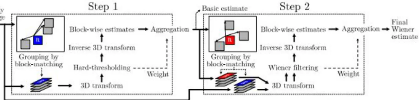
BM3D is a 2-step process and has been inspired by the non-local concept first introduced in

Non-Local Means (NLM). A block diagram illustrating the steps of BM3D is shown in Figure

2.3.

Figure 2.3: BM3D Block Diagram

In the first step, the process starts by defining a local neighborhood, also referred to as the

reference patch and searches for similar patches inside a search window, usually defined as

a bounded area around the reference patch. The similarity between the search patch and the

reference patch is decided based on a certain threshold. If the similarity is above the threshold,

(26)

be-tween the patches inside the bounded search area, all the similar patches are stacked together,

building a 3D block. BM3D applies some 3D transformations on the block to transform from

spatial domain to frequency domain. After the 3D transformation, the resulting coefficients are

thresholded, calledhard thresholding, where coefficients below a certain threshold are reduced

to zero. The block coefficients are transformed back to the spatial domain, using inverse 3D

transform. Next, BM3D generates a basic estimate of the denoised image from the block which

has been inverse transformed. For estimating the values of the reference patch, all the patches

in the 3D block are aggregated and it works by assigning different weights while estimating

the pixel values in the reference patch.

In the second step of BM3D another grouping of patches are carried out, similar to that

of the first step. This time however the grouping of patches into 3D blocks are done based

on the basic estimate obtained from the first step. After 3D blocks are generated by selecting

similar patches around the reference patch, the block is transformed using a 3D transformation.

Based on the transformed coefficients the restored image coefficients are estimated using the

restoration concept used in Wiener filter. The Wiener shrinkage coefficients are calculated for

the 3D blocks, followed by inverse transform to revert back to the spatial representation of the

3D block. Finally the Wiener shrinkage coefficients are multiplied by the 3D block to get the

(27)

2.4.4 BM3D Extensions

BM3D managed to demonstrate state-of-the-art performance compared to the previous

denois-ing models and after the method was initially proposed, researchers have continued to work

with the BM3D model to improve it’s denoising performance.

BM3D Denoising using Shape-Adaptive Principal Component Analysis

Dabov et al. proposed BM3D-SAPCA [7], an improvement over the regular BM3D using

shape adaptive image patches and applied Principal Component Analysis (PCA) on the

adap-tive shape neighborhood as part of the 3D transform on blocks. In the first step, it performs

shape adaptive grouping to find similar blocks and calculates the PCA basis of the 3D blocks.

The remaining steps, including 3D transform and hard thresholding, are carried out similar to

the one conventional BM3D.

BM3D Denoising using SSIM Optimized Wiener Filter

Hasan and El-Sakka [11] proposed an improvement in the Wiener filter optimized for

maximiz-ing the expected SSIM between the restored image and the original image. The improvement

in the underlying Wiener filter also helps to improve the performance of BM3D as it uses the

Wiener filter in the second phase of the denoising process. The main motivation was the

ob-servation that the mean squared error used in Wiener filter measures the absolute difference in

intensity between two images and it may occur than the mean squared error can have similar

values even when the two images are visually very different. To include some visual

infor-mation when denoising an image, the objective function of the Wiener filter is changed from

minimizing the expected MSE to maximizing the structural similarity between the restored and

(28)

2.5 Non-Local Means

Buades et al. proposed a non-local based approach for image denoising [3][4]. Images have

redundant or similar patterns in them and the Non-Local Means (NLM) approach attempts

to take advantage of such self-similarities to estimate the denoised gray value of each pixel.

Instead of using only a local region around each pixel for estimating the actual intensity of

the pixel, NLM uses a non-local approach by searching for similar patches, within a certain

search-bound, in the image. The center pixel of each patch contributes to a weighted averaging

based on the similarity between the reference and search patches.

When comparing the reference patch to a search patch, a variation of the Euclidean

dis-tance is measured. The Euclidean disdis-tance measures the sum of squared difference between

each pixel in a patch. To give more importance to pixels near the center of the patch, a

Gaus-sian weight distribution is used, thus resulting in the final measurement being the weighted

Euclidean distance,kN(i)−N(j)k2

2,a, wherea is the standard deviation of the Gaussian kernel

andN(i) andN(j) are the patches around pixeliand j, respectively. The weight associated with

each of the search patches is based on the similarity with the reference patch. After calculating

the Euclidean distance between the patches, the weight is assigned using:

w(i, j)= 1 Z(i)e

−

kv(_Ni)−v(_{N j})k2

2,a

h2 , (2.11)

whereZ(i) is the normalizing constant as defined by:

Z(i)=X j

e−

kv(_Ni)−v(_{N j})k2

2,a

h2 (2.12)

The constant,h, controls the decay rate of the exponential weight function. Given a noisy

image, the estimated valueNL[v](i), for pixeli, is computed as a weighted average of the center

(29)

NL[v](i)=X jI

w(i, j)v(j), (2.13)

wherew(i, j) is the weight calculated based on the similarity of neighborhood around pixel i

and j.

2.6 Non-Local Means Variants

The Non-Local Means(NLM) approach gained popularity due to its superior denoising results

compared to other existing spatial domain denoising models and researchers have continued

to work on the NLM approach to tackle some of it’s limitations. Some extensions have been

proposed to improve the computational cost.

2.6.1 Principal Components of Non-Local Means

Tasdizen used PCA to improve the computational time of non-local means [26]. The image

patches which are used in a given search space around a reference pixel are first projected

to a lower-dimensional subspace using PCA. The neighborhood similarity weights are then

calculated from the reduced subspace instead of the original full space. Let Mbe the number

of pixels in a neighborhood N and let {bp}M_p₌₁ be the eigenvector of the M × M empirical

covariance matrix for the set of all neighborhood vectors{v(N)j)} Q

j=1whereQdenotes the total

number of pixels in the image. The projections of the image neighborhood vectors onto the

d-dimensional PCA subspace is shown below:

v[d](Ni)= d

X

p=1

hv(Ni),bpi

| {z }

fp(Ni)

(30)

where fp(Ni) is the length of the ith vector’s projection onto the pth basic vector. Due to

or-thonormality of the basis

kv[d](Ni)−v[d](Nj)k2 =

d

X

p=1

(fp(Ni)− fp(Nj))2 (2.15)

The estimator fordis defined as:

ˆ

u[d](i)=X jSi

1 Zd(i)e

− Pd

p=1(fp(Ni)−fp(N j))2

h2 v(j) (2.16)

The proposed approach withd = Mis equivalent of the standard non-local means.

2.6.2 Improved Non-Local Means based on dimensionality reduction

Maruf and El-Sakka [20] proposed to improve the computational time of the original

non-local means algorithm by projecting image patches into a global feature space followed by

a dimensionality reduction using statistical t-test. In a preprocessing step, the global feature

space is generated by linearizing the patches to form a row vector of size j where j is the

number of pixels in the patch. The total size of the matrix C is N × j where N is the total

number of pixels in the image. After generating this matrix in the preprocessing step, a paired

t-test of the null hypothesis is computed on the matrix, where the hypothesis tries to accept or

reject a feature (i.e., an entire column in matrixC). After reducing the dimension of the initial

feature vector, the reduced vector is used for calculating the similarity between two patches.

The weighted averaging is based on the reduced feature space and thus reduces the exhaustive

search over all patches in a search region, as done in the standard non-local means method.

This achieves a reduction in the computation time of the algorithm.

Along with improvements in terms of the running time of the algorithm, the proposed

(31)

2.6.3 SSIM-based Non-Local Means

Rehman and Wang have proposed a SSIM based approach to non-local means [24]. For

calcu-lating the similarity between patches, the mean-squared error (MSE) may not always reflect the

true similarity between patches. As MSE measures the squared difference between the pixel

values, it may occur that two very different patches can have the same MSE values when

com-pared to the reference patch. The resulting denoised image may not have the best perceptual

quality. The SSIM-based approach uses the structural similarity to measure the likelihood of

similarity between the reference and the search patch. The weighted average is calculated as

shown:

ˆ X(i)=

P

jNiwS S I M(i, j)Y 0₍_j₎

P

jNiwS S I M(i, j)

, (2.17)

whereNidenotes the set of patches in the search area defined around pixeliandWS S I M(i, j) is

the SSIM weight between patchiand j.

The proposed method needed to address two major concerns. First, when calculating the

structural similarity between patches, especially in high noise levels, the SSIM value may end

up comparing the noise between the patches instead of the underlying structure. To overcome

this concern, the authors proposed a way to estimate the noise in the patches and deduct the

estimated noise from the pixel intensity values before calculating the structural similarity.

The second issue to address is that two structurally similar patches may have different

contrast and mean values. To avoid the bias in mean and contrast, the patches are normalized

before the weighted averaging step.

2.6.4 Iterative Non-Local Means

Bronx and Cremer [2] proposed an iterative non-local means approach. The non-local means

method is applied on an image in iterative mode. In each iteration, the similarity between

(32)

weights, the weighted averaging is done by multiplying the weights of a patch with it’s center

gray value in the noisy version of the image. The proposed method did well on regular

tex-tured image but in non-regular textex-tured image the resulting denoising image lost texture and

significant blurring is observed.

2.6.5 Non-Local Euclidean Median

Chaudhury and Singer [5] proposed the Non-Local Euclidean Median, extending the concept

of the original Non-Local Means scheme. The method is derived from the observation that the

median is more robust to outliers than the mean. In the presence of noise in the image, the

weights averaged over all possible patches, especially in a search-bound defined around image

edges and lines, will move the resulting mean towards the outliers. The mean is the minimizer

of P

jwjkP−Pjk2 over all patches P. Non-Local Euclidean Median proposed the select the

patch,P, which minimizesP

jwjkP−Pjkand replace the noisy pixel value at position (x,y) in the image with the pixel value of the center of patchP.

2.6.6 Two-stage Non-Local Means with adaptive smoothing parameters

Zhu et al. [33] proposed a two-stage non-local means method with adaptive smoothing

param-eters. Based on the noise estimation of a given noisy image, smoothing parameterhbasicfor the

first stage is selected automatically and the basic denoised image is computed, as shown:

ˆ yi,basic =

X

j

wi j,basicyj, (2.18)

wherewi j,basic is the weight depending on the similarity between patchesi and jand satisfies

the usual conditions 0 ≤ wi j,basic ≤ 1 andPjwi j,basic = 1. The weight is calculated as show in Equation (2.19)

wi j,basic =exp(− 1 h2

basic

(33)

wherePiandPjare the patches centered on pixeliand jandhbasicis the smoothing parameter

which controls the decay rate of the exponential function. For the first stage the smoothing

parameter is set ashi j,basic =0.75×σ.

Most of the image noise is removed after the first stage but for high noise levels some

noise artifacts still remain in the image, thus the basic image is refined one more time. The

resulting ˆybasicimage of the first stage is again denoised using the non-local means method but

using different smoothing parametershf inal. The final image is computed as shown in Equation

(2.20)

ˆ yi,f inal =

X

j

wi j,f inalyiˆ,basic (2.20)

Similar to the first stage, the weights between patchiand jare calculated as:

wi j,f inal=exp(− 1

h2_{f inal}kPi−Pjk

2₎ _(2.21)

In the second step of the process, the smoothing parameter is defined as:

hf inal =

           σ2

100, σ<30

0.5σ, σ≥ 30

2.7 Non-Local Means Applications

Non-local means and its variants have been used in various imaging applications such as

medi-cal imaging, including MRI brain images [13], CT scan imaging [15] and 3D ultrasound

imag-ing [12]. It is also used in video denoisimag-ing [10] [30], surface salinity detection [32] and metal

(34)

Methodology

The non-local means method defines a search area of sizeS ×S centered on the pixel,i, being denoised. The similarity of all the patches, defined around each of the pixels, within the search

area is considered during the weighted averaging process, where higher weights are assigned

to patches which are more similar, as determined by lower euclidean distance to the reference

patch. The goal of the weighted averaging process is to estimate the true noise-free intensity

value of pixeli, based on the similarity of the patches within the defined search area of a given

noisy image. The inclusion of center pixels of the patches which have low weights is likely to

deviate the resulting estimate from the true pixel intensity value of the denoised image.

3.1 Adaptive Non-Local Means using Weight Thresholding

In our proposed method, only a subset of the available patch centers are considered for the

estimation of the denoised pixel. The patches are selected based on the similarity measure

compared to the reference patch. Effectively, a cut-offweight,wthreshis selected using a defined

percentile value, wpercentile among the available patch weights within the bounded search area

and the weights of the patches are thresholded against wthresh. All weights above wthresh are

unchanged and weights below wthresh are reduced to zero, thus removing their pixel centers

(35)

from the weighted averaging process. The selected percentile is adjusted based on the noise

level of the given image. In real systems, the actual amount of noise in a noisy image cannot

be known beforehand. The noise can be estimated in digital image using fuzzy processing

techniques [25], image filters [21] and local variance estimate method [19]. In this research,

we used the local variance estimation method (see Section 2.1.1).

For low noise levels, a higher cut-offweight, wthresh, is selected for thresholding the patch

weights and as the noise level of a given image increases, wthresh is lowered to include more

patch centers for averaging. For lower noise levels, only the patches with high similarity

mea-sure to a reference patch can be used to estimate a denoised image. The remaining patches can

be considered outliers. So, a higher cut-offthreshold is selected for low noise levels. In high

noise, the Euclidean distance measurement may not give a true measure of patch similarity as it

will end up comparing, to some extent, the noise between patches along with the structures of

the patches. So, considering only the higher weighted patch centers, by keeping the threshold

value high, can in fact deviate the denoised estimation from the true value. To mitigate this

effect, the threshold value is lowered so that more pixels are averaged for attenuating the noise.

The denoised image is calculated as shown below:

NL[v](i)=X jI

ˆ

w(i, j)v(j), (3.1)

where ˆw(i, j) is the thresholded weight between patch at pixeliand patch at pixel jas shown:

ˆ w(i, j)=

              

w(i, j), ifw(i, j)>wthresh

0, otherwise

(3.2)

Non-local means has two key parameters, namely the patch size and the search size. These

parameters are kept constant irrespective of the amount of noise in the image. In our proposed

(36)

noise level in the image. Through a iterative learning approach, we have empirically defined

models for selecting the patch size and the corresponding search window size for any noise

level, σ. The models were determined empirically using an iterative learning approach on a

training image set.

The proposed method is applied in a two-step approach. In the first step, the proposed

method is used to generate a basic estimate of the denoised image. In the basic estimate, most

of the noise is reduced but still some visible noise artifacts remain, especially for stronger noise

levels and it is necessary to further denoise the basic image for better denoising [31]. As most

of the noise is reduced in the basic image, similar regions can be identified more easily which

helps to generate better denoised images in the second step. In the second step, the basic image

is denoised using a similar method utilized in the first step, but with smaller smoothing

param-eters. To verify that the two-step approach is sufficient, we conducted experiments to measure

the improvement in the denoising performance with further steps and found the amount of

improvements to be negligible. The results of this experiment is shown in Section 3.2.3

3.2 Parameter Selection

The primary parameters in the proposed method are:

1. Cut-offweight for thresholding

2. Patch size

3. Search window size

The parameters are determined empirically, based on experiments conducted on a set of test

images. The performance measure of tuning each of the parameters are used to define the

mod-els for the parameters. The set of test of images is shown in Figure 3.1. The training images are

(37)

and fine details. The Lena and Peppers images have smooth regions, while Barbara, Boats

and Baboonimages has lot more texture and fine details. All the PSNR values reported are

averaged after repeating each of the experiments 10 times.

(a) (b)

(c) (d) (e)

Figure 3.1: Training image set (a) Lena. (b) Barbara (c) Peppers (d) Baboon (e) Boats

3.2.1 Cut-o

ff

Weight for Thresholding

The patch size and search window size are fixed and the weights are thresholded based on the

cut-offweight percentile,wpercentile, determined by the model. For the purpose of determining

(38)

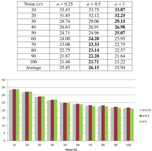
Table 3.1: PSNR Comparison of linear models for different coefficienta

Noise (σ) a= 0.25 a=0.5 a=1

10 33.43 33.75 33.87

20 31.85 32.12 32.25

30 28.74 29.06 29.15

40 26.63 26.91 26.98

50 24.71 24.96 25.07

60 24.00 24.28 23.95

70 23.08 23.33 22.75

80 22.75 23.14 22.57

90 21.87 22.28 21.64

100 21.48 21.71 21.22

Average 25.85 26.15 25.94

Figure 3.2: Bar chart of PSNR for different linear models (changing the coefficienta)

Linear Model

The linear model for determining the cut-offweight percentile is defined as:

wpercentile =ceil(100−aσ), (3.3)

whereceil() rounds a decimal value to the smallest following integer, coefficientais a constant

andσis the standard deviation of Gaussian noise.

(39)

comparison of using different linear models for weight thresholding is tabulated in Table 3.1.

Figure 3.2 shows the bar chart of PSNR comparison between various linear models. For noise

levelsσ≤ 50, a coefficient value ofa= 1 generate better results and forσ>50, the coefficient valuea=0.5 demonstrate better performance.

Exponential Model

The exponential model for determining the cut-offweight percentile is defined as:

w

percentile

=

ceil

(100

×

e

−0.01aσ

₎

_,

_(3.4)

whereceil() rounds a decimal value to the smallest following integer, coefficientais a constant

andσis the standard deviation of Gaussian noise.

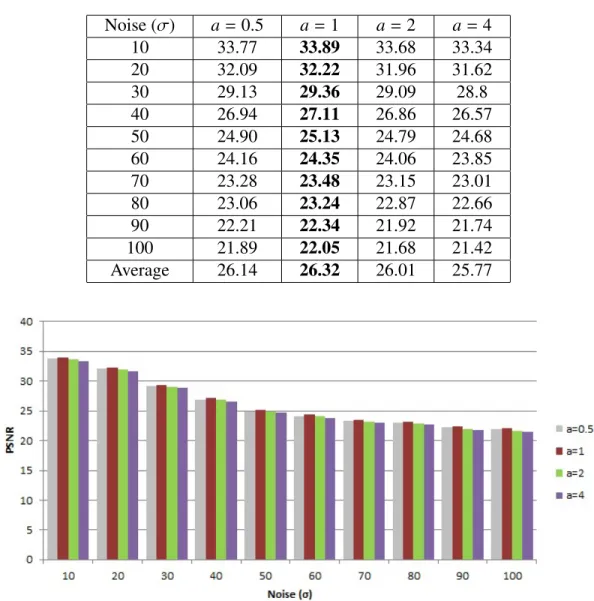
The result of using the exponential model for determining the cut-off weight is shown is

Table 3.2. Figure 3.3 shows the bar chart of PSNR comparison between different exponential

models. For the exponential model, the coefficient value of a = 1 demonstrate better results

for all noise levels. The average performance, as well as the noise-wise performance, of the

exponential model, with coefficienta = 1, has better denoising performance compared to the

linear models. So, the exponential model, with coefficienta=1 is selected for determining the

cut-offweight percentile for any given noise level,σ.

3.2.2 Patch Size and Search Window Size

For varying the search window size, the patch size is fixed at 7×7. The weights are thresholded using the exponential model, selected in previous section. The result of varying the search

window is shown in Table 3.3. The table shows that forσ<50 the search window size 11×11

perform optimally and forσ ≥ 50 the search size 21×21 performs best. To help determine

(40)

Table 3.2: PSNR Comparison between exponential models for different coefficienta

Noise (σ) a=0.5 a=1 a= 2 a= 4

10 33.77 33.89 33.68 33.34

20 32.09 32.22 31.96 31.62

30 29.13 29.36 29.09 28.8

40 26.94 27.11 26.86 26.57

50 24.90 25.13 24.79 24.68

60 24.16 24.35 24.06 23.85

70 23.28 23.48 23.15 23.01

80 23.06 23.24 22.87 22.66

90 22.21 22.34 21.92 21.74

100 21.89 22.05 21.68 21.42

Average 26.14 26.32 26.01 25.77

Figure 3.3: Bar chart of PSNR comparison between different exponential models (changing

coefficienta)

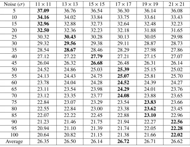
are again measured by varying the search window size, but this time using odd-integer window

sizes only between 11×11 and 21×21, while using more noise levels.

The patch size and search window size for a given noise level are determined empirically,

using an iterative learning approach on a training image set. At first, the patch size is fixed

and the search window size is varied, for each noise levels, to select the best search window

size. The noise levels, σ, ranges from 10 to 100, with a step size equals 5. Next, the patch

(41)

Table 3.3: PSNR Comparison by changing the search window size

Noise (σ) 5×5 11×11 21×21 35×35

10 33.26 34.19 33.94 33.40

20 31.44 32.48 31.66 31.28

30 28.83 29.35 28.68 28.27

40 27.44 28.12 28.06 27.44

50 23.79 24.56 25.05 24.40

60 22.84 23.70 24.27 23.91

70 22.15 23.09 23.73 23.48

80 21.66 22.56 23.41 23.19

90 20.73 21.57 22.88 22.42

100 20.35 21.06 22.52 22.15

Average 25.25 26.07 26.42 25.99

Figure 3.4: Bar chart of PSNR comparison between different search window size

determined in the previous step. The best patch size for each noise level is used to find the

corresponding optimal search window sizes one more time. This process is repeated until an

iteration is reached where updating the optimal search window size for a noise level did not

change the corresponding best patch size and vice versa.

To determine the patch and search window size models, the patch size is initially fixed at

7× 7 and the search window size is varied. The average PSNR comparison of the various

(42)

Table 3.4: PSNR Comparison for fine tuning the search window size

Noise (σ) 11×11 13×13 15×15 17×17 19×19 21×21

5 37.09 36.76 36.54 36.30 36.14 36.08 10 34.16 34.02 33.84 33.75 33.61 33.43 15 32.96 32.88 32.73 32.64 32.48 32.23 20 32.50 32.36 32.23 32.18 31.88 31.65

25 30.32 30.43 30.28 30.13 30.05 29.98

30 29.32 29.56 29.38 29.11 28.87 28.73

35 28.54 28.67 28.46 28.29 27.98 27.86

40 27.12 27.22 27.79 27.21 27.15 27.07

45 26.04 26.32 26.68 26.48 26.31 26.14

50 24.52 24.86 25.03 25.39 25.15 25.02

55 24.13 24.43 24.75 25.07 25.81 25.70

60 23.78 24.04 24.28 24.52 24.39 24.27

65 23.11 23.54 23.98 24.29 24.01 23.76

70 23.12 23.35 23.77 24.08 23.88 23.65

75 22.84 23.07 23.29 23.54 23.83 23.66

80 22.55 22.84 23.00 23.38 23.62 23.45

85 22.07 22.22 22.45 22.88 23.10 22.96

90 21.23 21.46 21.75 21.94 22.27 22.56

95 20.94 21.10 21.39 21.74 22.05 22.28

100 20.64 20.82 21.15 21.38 21.66 22.02

(43)

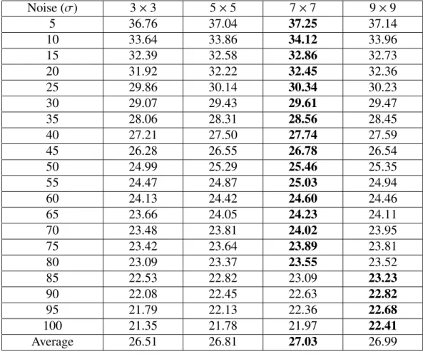
Table 3.5: PSNR Comparison by changing the patch size

Noise (σ) 3×3 5×5 7×7 9×9

5 36.76 37.04 37.25 37.14

10 33.64 33.86 34.12 33.96

15 32.39 32.58 32.86 32.73

20 31.92 32.22 32.45 32.36

25 29.86 30.14 30.34 30.23

30 29.07 29.43 29.61 29.47

35 28.06 28.31 28.56 28.45

40 27.21 27.50 27.74 27.59

45 26.28 26.55 26.78 26.54

50 24.99 25.29 25.46 25.35

55 24.47 24.87 25.03 24.94

60 24.13 24.42 24.60 24.46

65 23.66 24.05 24.23 24.11

70 23.48 23.81 24.02 23.95

75 23.42 23.64 23.89 23.81

80 23.09 23.37 23.55 23.52

85 22.53 22.82 23.09 23.23

90 22.08 22.45 22.63 22.82

95 21.79 22.13 22.36 22.68

100 21.35 21.78 21.97 22.41

Average 26.51 26.81 27.03 26.99

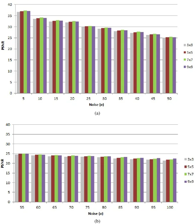
For the next step of determining the patch size to be used in our proposed method, the patch

size is varied while using the optimal search window for a given noise level, as shown in Table

3.3. The result of changing the patch size is shown in Table 3.5. The results indicated that the

patch size 7×7 works optimally for noise levelσ<85 and for noise levelσ≥ 85 the patch size 9×9 is optimal.

For noise levelσ≥ 85, the optimal patch size is different than the patch size used to find the optimal search window size previously. The experiment for finding the optimal search window

is again iterated, but this time only for noise levelsσ ≥ 85 and using a patch size 9×9. The PSNR comparison is shown in Table 3.6.

As the optimal search window size did not change, even with the updated patch size, the

(44)

(a)

(b)

Figure 3.5: PSNR comparison between different patch sizes (a) Noise,σ 5 - 50 (b) Noise, σ

(45)

Table 3.6: PSNR Comparison by fixing patch size=9×9 and changing search window size

Noise (σ) 11×11 13×13 15×15 17×17 19×19 21×21

85 22.28 22.51 22.74 23.02 23.27 23.14

90 21.53 21.75 22.02 22.21 22.54 22.85

95 21.24 21.47 21.82 22.19 22.48 22.64

100 21.17 21.32 21.65 21.86 22.11 22.43

Average 21.55 21.76 22.06 22.32 22.60 22.76

The optimal search window sizes and the corresponding noise levels are plotted in a graph,

as shown in Figure 3.6. The plotted points are used to determine a model, for the search

window size, using a best-fit curve for the given points. Three different models are used to

determine the best-fit curve:

1. Linear Model

2. Quadratic Model

3. Exponential Model

The best fit curve using a linear model is shown in Figure 3.7. The best fit curve for the

quadratic model is shown in Figure 3.8 and the curve for the exponential model is shown in

(46)

Figure 3.6: Plot of optimal search window for various noise levels

(47)

Figure 3.8: Curve fitting using a quadratic model

(48)

The goodness of each of the curve models is evaluated using the R-squared statistical

mea-sure. It measures how close the actual data points are to the fitted curve and the values range

from 0.0 to 1.0, where a higher value represents a better-fit curve. The equations and the

R-squared values of the three models are:

1. Linear Model: y= 0.117σ+9.758, R2 = 0.965

2. Quadratic Model:y= −0.0001σ2+0.127σ+9.574, R2 =0.965 3. Exponential Model:y= 10.409e0.008σ, R2 =0.952

Based on the R-squared values, the linear and quadratic models have very similarR2_results.

In the quadratic model, the coefficient of the x2term is close to 0, making the model equation

very similar to the linear model. The R-squared value of the exponential model is lower than

that of the linear model and exponential functions are more computationally expensive than

linear functions. Comparing the curve fittings of the three models, the linear model is selected

for determining the search window size for any given noise levelσ.

As the search window is centered around the pixel being denoised, it is required to use

odd-numbered size for the search. For a given noise level, the result of the linear model is

rounded to the nearest odd number to be used as the search window size. The search window

size model is defined as:

S = roundodd(0.117σ+9.758) (3.5)

where, roundodd() rounds to the nearest odd integer andS ×S is the dimension of the search

window.

3.2.3 The two-step approach

Using the patch and search window size models along with the exponential weight thresholding

(49)

Table 3.7: PSNR comparison of proposed method for multiple steps for various noise levels

Noise Level 1 step 2 step 3 step 4 step

10 34.11 34.16 33.71 33.56

20 32.43 32.70 32.31 32.23

30 29.55 29.86 29.47 29.34

40 27.78 28.29 27.92 27.83

50 25.44 26.10 25.77 25.69

60 24.66 25.42 25.18 25.08

70 23.99 24.88 24.73 24.66

80 23.61 24.62 24.48 24.30

90 22.79 23.96 23.99 23.85

100 22.48 23.76 23.80 23.68

Average 26.68 27.37 27.14 27.02

Figure 3.10: Bar chart of PSNR comparison of proposed method for multiple steps

In each step, the proposed method was applied on the output image of the previous step. After

each iteration, the PSNR of the resulting denoised image was measured. The change in the

PSNR measurement, compared to the previous iteration, was used to determine the number of

iterations which demonstrated satisfactory performance improvement due to the extra iteration.

The PSNR comparison of multiple iterations of the proposed method is shown in Table 3.7. The

(50)

3.3 Summary of the selected parameters

The key parameters of the proposed method were empirically defined using different models.

The percentile of cut-offweight used for thresholding is defined as:

w

percentile

=

ceil

(100

×

e

−0.01aσ

₎

_(3.6)

The patch-size,P×P, is selected as shown below: P=               

7 ifσ<85

9, otherwise

(3.7)

The search window size,S ×S is determined as:

(51)

Experimental Results and Analysis

The proposed image denoising method has been tested on the standard Kodak image set. The

images are corrupted with additive white Gaussian noise with the noise level (standard

devia-tion), σranging from 10 to 100, with step size equals 10. The proposed method is compared

with the original non-local means scheme, variants of non-local means and the BM3D method.

4.1 Image set

All the experiments are carried out of the standard Kodak gray-scale image set. It comprises of

24 gray-scale images of dimensions 768×512 and 512×768. The images in the Kodak image

set are shown in Figure 4.1. The standard images are noise-free and additive white Gaussian

noise is added on top of the noise-free image to generate the noisy image.

4.2 Noise Generation

The additive noise signal is added to the original noise-free signal in order to generate the noisy

signal. For the purpose of our experimentation, the standard noise-free image are contaminated

by adding Gaussian white noise, distributed throughout the image. The final intensity values

(52)

(a) Windows (b) Door (c) Hats (d) Bike

(e) Lake (f) Flower (g) Houses (h) Bridge

(i) Beach (j) Landscape (k) Raft (l) Girl

(m) Island (n) Plane (o) Lighthouse (p) House

(q) Parrot (r) House 2

(s) Sail (t) Boat 2

(u) Statue (v) Model (w) Lighthouse 2 (x) Woman

(53)

(a) Original Image (b) Noisy Image

Figure 4.2: Example of Gaussian noise (σ=40) added to a noise-free image

were kept within the maximum intensity value of gray-scale images. In our experiments, all

the noisy images are generated inMAT LABusing the following method:

imNoise

=

im

+

(

₂₅₅σ

×

randn

(

size

(

im

)))

,

where

imNoise

is the noisy image,

im

is the original, noise-free image,

σ

is

the required noise level and the function

randn

() generates a random matrix

with Gaussian distribution and size equal to the dimension of the original input

image.

An example of additive white Gaussian noise added to a noise-free image is

shown in Figure 4.2

4.3 Performance Measure

To measure the performance of our proposed method in comparison to other

ex-isting denoising methods, we have used the Peak Signal to Noise Ratio (PSNR)

and the Mean Structural SIMilarity (MSSIM) measure. These measures are

(54)

denois-ing methods. We also performed subjective comparison between our proposed

method and existing denoising methods.

4.3.1 Peak Signal to Noise Ratio (PSNR)

The Peak Signal to Noise Ratio measures the ratio between the maximum

pos-sible power of a signal to the power of the noise which a

ff

ects the quality of

the original signal. The PSNR is usually expressed as the logarithmic

deci-bel scale. A higher value in PSNR represents better reconstructed or denoised

image. The PSNR is measured using:

PS NR

=

10 log

₁₀

(

MAX

2

I

MS E

)

,

(4.1)

where

MAX

I

represents the maximum intensity of the image and

MS E

mea-sures the mean squared error between the original image and the degraded

im-age, defined as:.

MS E

=

1 M

×

N

M

X

i=0

N

X

j=0

(

u

i j

−

v

i j

)

2

,

(4.2)

where

u

i j

is the original image,

v

i j

is the degraded image and the size of the

images is

M

×

N

.

4.3.2 Mean Structural Similarity (MSSIM)

One of the drawbacks of the PSNR measure is that it relies on the mean square

(55)

er-ences between isolated data points. To evaluate the performance of a denoising

method based on the degree of structural similarity between the original and

the reconstructed image, the Structural SIMilarity (SSIM) measure can be used

[27][28]. The SSIM measure provides a better assessment of an image

restora-tion or denoising method. The SSIM between two blocks is defined as:

S S I M

=

(2

µ

x

µ

y

+

c

1

)(2

σ

xy

+

c

2

)

(

µ

2

x

+

µ

2y

+

c

1

)(

σ

2x

+

σ

2y

+

c

2

,

(4.3)

where,

x

and

y

are two identical sized window or patch,

µ

x

and

µ

y

are the

averages of

x

and

y

,

σ

2_x

and

σ

2_y

are the variance of

x

and

y

and

σ

xy

is the

co-variance. The mean SSIM (MSSIM), averaged over all SSIM, is used as for the

(56)

4.4 Results and Analysis

The proposed method is compared with the original

Non-Local Means

(NLM)

scheme, the

Two-Stage Non-Local Means

(TS-NLM) scheme , the

Non-Local

Euclidean Median

(NLEM) scheme and the

Block Matching and 3D Filtering

(BM3D) scheme. All the objective measurements reported are averaged after

repeating each of the experiments 10 times. The denoising performances are

compared after running each of the denoising methods, including the proposed

method, on the same noisy image for each noise level,

σ

.

4.4.1 Performance evaluation using PSNR

Table 4.1 shows the PSNR comparison for the

Girl

image and Table 4.2 shows

the average PSNR values over all images in the Kodak image set, for various

noise levels. Figure 4.3 shows the bar chart of PSNR comparison among the

proposed method and existing denoising methods, for various noise levels. The

PSNR values are reported after averaging the results of 10 runs. The standard

deviation of PSNR for each of the noise levels is shown in Table 4.3.

The performance of the proposed method is better than the original

non-local means method and its variant for all noise levels. Yet, when compared

to BM3D, our proposed method managed to produce better results only when

σ

≤

80. The proposed method also demonstrated better performance than

(57)

Table 4.1: PSNR comparison of theGirlimage among the proposed method, the NLM method, variants of NLM and BM3D denoising scheme for various noise levels

Noise Level NLM TS-NLM NLEM BM3D Proposed

10 33.92 33.93 32.90 35.42 35.61

20 31.83 32.01 31.85 33.46 33.60

30 29.43 29.70 29.56 31.03 31.12

40 28.47 28.96 28.61 29.88 30.04

50 26.64 27.20 26.98 28.21 28.27

60 25.12 25.77 25.30 26.53 26.60

70 24.78 25.24 25.01 25.88 26.03

80 23.69 24.46 23.93 25.33 25.50

90 23.15 24.04 23.52 24.95 24.81

100 22.91 23.88 23.18 24.43 24.28

Average 26.99 27.52 27.08 28.51 28.59