Issues in Dimensionality Reduction of
Multispectral and Hyperspectral data.
Bijith Marakarkandy,Dr. B.K. Mishra TCET, Mumbai,India.
Abstract-The focus of this paper is to examine ways to perform analysis of Multispectral and Hyperspectral data in order to understand the issues involved in dimensionality reduction of this data. This paper proposes ways to examine the data using different techniques so that an informed decision can be arrived upon while choosing the dimensionality reduction methods.
Keywords – Hyperspectral data compression, Multispectral data,
PCA, MNF, PPI.
I. INTRODUCTION
Observing the earth by remote sensing provides a global picture of the earth. This has wide spread use for military and civilian purpose. Remote sensing can be defined as measuring the properties of an object without actually looking at the objects physical characteristic i.e. without any physical contact. When the solar energy is incident on an object, some of it is reflected, some energy is emitted and some of the energy is absorbed while some of the energy is transmitted. Every material has a unique spectral signature. The manner in which an object reflects energy depends primarily on its optical properties. The goal of collecting spectral image data is to extract signatures for material detection, classification, identification, characterization and quantification.
II. LANDSAT 7
Landsat 7 was launched on April 15th 1999. The goal of Landsat 7 is to refresh the global archive of satellite images, providing up-to date and cloud free image. The altitude of Landsat 7 is approximately 705 Km with recurrence period of 16 days. The Landsat 7 carries an enhanced TM sensor know as Enhanced Thematic Mapper plus (ETM +)
The Thematic Mapper (TM) is an advanced Multispectral scanning, earth resources sensor designed to achieve higher image resolution, TM are sensed in seven spectral bands simultaneously. Band 6 senses thermal (heat) infrared radiation. Landsat can only acquire night scenes in Band 6. A TM (Thematic Mapper) has instantaneous field of view (IFOV) of 30 sq m in Band 1-5 and 7 while Band 6 has an IFOV of 120 sq m on the ground.
A. Thematic Mapper (TM) Bands:
Band Number μm Resolution Spectral
Response
1 0.45-0.52 30m Blue-Green
2 0.52-0.60 30m Green
3 0.63-0.69 30m Red
4 0.76-0.90 30m Near IR
5 1.55-1.75 30m Mid IR
6 10.4-12.5 120m Thermal IR
7 20.8-23.5 30m Mid IR
The Enhanced Thematic Mapper (ETM) has an additional panchromatic band.
Band 8: 0.52-0.90 µm with 15m resolution.
B. Different Formats to Store the Raster Data Band Interleaved Format (BIL).
The first line of the first band is stored, followed by the first line of the second band, followed by the first line of the third band, subsequent lines are interleaved in similar fashion. This type of format provides a compromise in performance between spatial & spectral processing.
Band Sequential Format (BSQ).
In this format each line of the data is followed immediately by the next line in the same spectral band. This format is the best for spatial (x, y) access of any pixel of a spectral band.
Band Interleaved By Pixel Format (BIP).
In this format the first pixel for all bands is in sequential order followed by the second pixel for all bands, by the second pixel for all bands, followed by the third pixel of all bands, and so forth, it is interleaved up to the number of pixels. This format is best suited for spectral access of the image data
C. Description of the various Bands:
Band-1: Coastal water mapping, soil/vegetation discrimination, forest classification, man-made feature identification.
Band-2: Vegetation discrimination and health monitoring, man-made feature identification.
Band-3: Plant species identification, man-made feature identification.
Band-4: Soil moisture monitoring, vegetation monitoring, and water body discrimination.
Band-5: Vegetation moisture content monitoring.
Band-6: Surface temperature, vegetation stress monitoring, soil moisture monitoring, cloud differentiation, volcanic monitoring.
Band-7: Mineral and rock discrimination, vegetation moisture content.
III. AVIRIS
HYPERSPECTRAL IMAGES
Hyperspectral remote sensing combines imaging and spectroscopy in a single system. Hyperspectral data sets are generally composed of about 100 to 200 spectral bands of relatively narrow bandwidths (5-10 nm) whereas, Multispectral data sets are usually composed of about 5 to 10 bands of relatively large bandwidths (70 – 400 nm)
Hyperspectral data can be represented using a cube or it can also be thought of as an n-dimensional scatter plot. The data for a given pixel corresponds to a spectral, reflectance for a given pixel.
Fig 1: 3D surface view of a Hyperspectral Image showing elevation.
The following table can be used to compare Multispectral and Hyperspectral images.
MULTISPECTRAL HYPERSPECTRAL Separated spectral bands. No gaps
Wider Bandwidths Narrow Bandwidths Coarse representation of the
spectral signatures
Complete representation of the spectral signatures
Small image size Large image size
IV. CREATING COLOR COMPOSITE OF MULTISPECTRAL IMAGES
Satellites acquire images in black and white. We can assign false colors to those black & white images.
The three primary colors red, green and blue can be displayed in three different bands at a time by using a different primary color for each band. When we combine these three images we get a “False Color Image “.
To make a color composite RGB = NRG Red = Near IR (Band-4) Green = Red (Band-3) Blue = Red (Band-2)
Vegetation appears as shade of red soil with little or no vegetation will range from white (for sand) to green and brown depending upon the moisture and organic matter content.
Water will range form blue to black. Clear deep water is dark and sediment laden or shallow water appears lighter.
Urban areas look blue-gray.
Clouds and snow both of them appear to be white in color. We have written a code in matlab that displays a LANDSAT image and the corresponding scatter plot of the 3-bands. We find that there are a number of pixels along the diagonal which is typical of urban areas.
Fig 2: Landsat image of Bombay city with bands 3 2 1 shown as RGB image and its scatter plot is displayed on the right. False Color Satellite images can yield valuable information
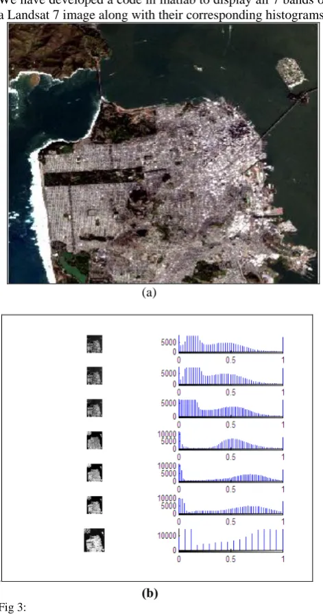
We have developed a code in matlab to display all 7 bands of a Landsat 7 image along with their corresponding histograms.
(a)
.
(b) Fig 3:
(a) Landsat 7 image of San Francisco City
V. MULTISPECTRAL IMAGE ANALYSIS A. NDVI
The “Normalized Difference Vegetation Index (NDVI)” is a calculation, based on several spectral bands of the photosynthetic output in a pixel in a satellite image.
NDVI = NIR – RED
NIR + RED
The value of this index varies from -1 to +1. the common range for the green vegetation is 0.2 to 0.8.
B. EVI
The “Enhanced Vegetation Index” was developed to improve the NDVI by optimizing the vegetation signal in LAI regions by using the blue reflectance to correct for soil background signals and reduce atmospheric influences including aerosol scattering.
EVI = (2.5) x NIR – RED . NIR – 6 RED – 7.5BLUE + 1
The value of this index ranges from -1 to +1. The common range for green vegetation is 0.2 to 0.8
We have developed a code in matlab to display a Landsat image along with its NIR v/s RED scatter plot.
This program also displays an image with vegetation shown as green by applying a threshold to NDVI. The program also computes the percentage of pixels which represent vegetation.
(a)
(b)
Fig 4:
(a) Landsat 7 image of a paddy field.
(b) Its scatter plot of NIR v/s RED and the resulting image after applying the threshold of 0.40.
When a threshold of 0.40 was applied Percentage of pixels corresponding to vegetation is 54.3678
VI. DIMENSIOANLITY REDUCTION OF MULTISPECTRAL AND HYPERSPECTRAL
DATA
A. Minimum Noise Fraction (MNF)
This can be used to determine the inherent dimensionality of image data, to segregate noise in the data and to reduce computational requirements for subsequent processing. We can use the MNF transform for noise removal by first performing a forward transform, and finding out which bands contain the coherent images and then using an inverse MNF transform using only good bands.
B. Pixel Purity Index (PPI)
It is an End Member Extraction Algorithm (EEA) developed by Boardman et al. It is designed to search for a set of vertices of a convex geometry in a given data set that are supposed to represent pure signatures present in the data.
C. Band Ratios
Band ratios are used for enhancing the spectral differences between bands. When we divide one spectral band by another, the resulting image enhances the spectral differences between the bands.
We have written a code in Matlab to display Landsat 7 image. The program allows the user to select the bands and compute the band ratio and it displays the resulting image.
Fig 5: Landsat 7 image of San Francisco with Bands 3 2 1 on left and Band ratio image of Band 7 and Band 5 of image is shown on the right side.
We have selected an image of Bangalore city (India) for dimension reduction. The image has 6 bands and the information about it is provided below:
Mapinfo: Proj UTM Zone 43N Pixel 28.5m Datum: WGS-84
Fig6: Landsat 7 image of Bangalore City
(The authors acknowledge the contribution of socioeconomic data and application center (SEDAC) at Center for International Earth Science Information Network (CIESIN) of Columbia University for permission to use the raw data of Bangalore city)
We are using a software ENVI (Environment for the visualization of images) from RSI which is used by the AVIRIS data facility (ADF) by NASA at the Jet propulsion laboratory California institute of technology for this work. Our aim is to find and map spectral end members from the image, we will be applying MNF transformation to reduce spectral dimension. We will determine the dimensionality of the data using spatial coherence methods. We will also calculate the PPI to reduce spatial dimensions.
Mask band selected is band 6
The MNF transform when applied to the image uses two cascaded Principal Component Transformations. The first transformation estimates a noise covariance matrix, decorrelate and rescale the noise in the data. The resulting data has noise which has unit variance and no band-to-band correlations. The next transform is a normal Principal Component Transformation of noise-whitened data. The resulting bands of the MNF transformed data are ranked in decreasing order of variance. The last few bands are therefore noisy.
The figure 7 shows a plot of eigenvalue v/s eigen number of the MNF of image of Bangalore city.
Fig 7: Eigen value plot of MNF
The MNF eigenvalue plot shows the eigenvalue for each MNF transformed band. (Eigenvalue Number) larger eigenvalue indicate higher data variance in the transformed band. When eigenvalues approach 1 only noise is left in the transformed band.
The first 3 MNF bands as RGB are shown below. These can be used for location of dominant spectral materials.
Fig 8: MNF band 1, band 2 and band 3 shown as RGB image.
Signal to noise ratio decreases as the MNF band number increases
(a) (b)
(c) (d)
(e) (f)
Dimensionality reduction can be achieved by dividing the MNF images into two classes’ one class with larger eigenvalues, and another class with near unity eigenvalues (i.e. noise dominated)
Fig 10: Plot of MNF band number v/s spatial coherence value
The user can use only the coherent portions by thresholding the MNF bands.
We choose a threshold of 0.45.
The number of bands above this threshold is 5
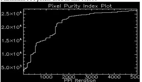
Pixel Purity Index (PPI) is used to find the most “spectrally pure” or extreme pixels in the data. The PPI is computed by repeatedly projecting n-dimensional scatter plots onto a random unit vector. The extreme pixels in each projection are recorded and the total number of times each pixel is marked as extreme is noted.
A threshold is selected which is approximately 2-3 times the noise level in the data.
Maximum PPI pixels used in this 10,000
Fig 11: Plot of PPI (Pixel Purity Index)
VII. CONCLUSION
We have investigated Multispectral and Hyperspectral images. The dimensionality determination is little tricky issue and many a times we have to resort to a generous estimate. We have to use MNF bands that have a reasonable image quality determined by its eigenvalues above one. The process of choosing the dimensionality is scene dependent. There is a scope for future work to decorrelate each band by applying an orthogonal transform and bands in which there is a high degree of correlation can be subjected to dimensionality reduction techniques proposed in this paper.
REFERENCES
[1]. Qian Du and J.E.Fowler, “Hyperspectral Image Compression using JPEG-2000 and Principal Component Analysis” IEEE Geosci. Remote Sens. Lett. Vol.4 no2, Apr.2007
[2]. NASA, 2007, http://www.nasa.gov/centres/goddard/home/index.html [3]. Osmar Abilio de Carvalho Jr, et al, “Sequential Minimum Noise Fraction use: AN approach to noise elimination”
[4]. Chein-I Chan and Qian Du, “Estimination of number of spectrally distinct signal sources in Hyperspectral Imagery” IEEE Trans. Geosci Remote Sensing PP.608-619 vol.42, No.3. March 2004
[5]. Socioeconomic data and application, 2007,http://sedac.ciesin.org [6]. Chein-I Chan and Su Wang, “Constrained band selection for Hyperspectral Imagery” IEEE Trans. Geosci remote Sensing PP.1575-1585 vol.44, No.6, June 2006.