Western University Western University
Scholarship@Western
Scholarship@Western
Electronic Thesis and Dissertation Repository
4-16-2013 12:00 AM
NFA reduction via hypergraph vertex cover approximation
NFA reduction via hypergraph vertex cover approximation
Timothy Ng
The University of Western Ontario
Supervisor
Dr. Roberto Solis-Oba
The University of Western Ontario Graduate Program in Computer Science
A thesis submitted in partial fulfillment of the requirements for the degree in Master of Science © Timothy Ng 2013
Follow this and additional works at: https://ir.lib.uwo.ca/etd
Part of the Theory and Algorithms Commons
Recommended Citation Recommended Citation
Ng, Timothy, "NFA reduction via hypergraph vertex cover approximation" (2013). Electronic Thesis and Dissertation Repository. 1224.
https://ir.lib.uwo.ca/etd/1224
This Dissertation/Thesis is brought to you for free and open access by Scholarship@Western. It has been accepted for inclusion in Electronic Thesis and Dissertation Repository by an authorized administrator of
(Thesis format: Monograph)
by
Timothy Ng
Graduate Program in Computer Science
A thesis submitted in partial fulfillment
of the requirements for the degree of
Master of Science
The School of Graduate and Postdoctoral Studies
The University of Western Ontario
London, Ontario, Canada
Abstract
In this thesis, we study the minimum vertex cover problem on the class of k-partite k
-uniform hypergraphs. This problem arises when reducing the size of nondeterministic
finite automata (NFA) using preorders, as suggested by Champarnaud and Coulon. It
has been shown that reducing NFAs using preorders is at least as hard as computing a
minimal vertex cover on 3-partite 3-uniform hypergraphs, which is NP-hard. We present
several classes of regular languages for which NFAs that recognize them can be optimally
reduced via preorders. We introduce an algorithm for approximating vertex cover on
k-partite k-uniform hypergraphs based on a theorem by Lovász and explore the use of
fractional cover algorithms to improve the running time at the expense of a small increase
in the approximation ratio.
Keywords: regular languages, vertex cover, approximation algorithms, nondeterministic finite automata, approximate fractional covering, NFA reduction
I would like to thank Roberto Solis-Oba for his supervision, for encouraging me to work
on what I was interested in, and for his advice and guidance, which helped shape this
work.
I would like to thank my initial advisor, Sheng Yu, who sadly passed away, for
en-thusiastically guiding me through the early part of my graduate studies.
And finally, I would like to thank my family for the support they have given me
throughout my studies.
Contents
Abstract ii
Acknowledgements iii
List of Figures vi
List of Tables vii
1 Introduction 1
2 Regular Languages 4
2.1 Preliminaries . . . 4
2.2 Regular expressions . . . 5
2.3 Finite automata . . . 6
2.4 Converting regular expressions to finite automata . . . 10
3 The Vertex Cover Problem 13 3.1 Complexity theory . . . 13
3.2 The minimal vertex cover problem . . . 14
3.3 Approximation Algorithms . . . 17
4 The NFA reduction problem 21 4.1 Preliminaries . . . 21
4.1.1 Reducing NFAs based on equivalences . . . 22
4.1.2 Reducing NFAs based on preorders . . . 24
4.2 Complexity of computing pre-reduced NFAs . . . 28
5 An approximation algorithm based on Lovász’s theorem 34 5.1 Lovász’s theorem . . . 34
5.2 The algorithm . . . 37
5.3 Applying Lovász’s theorem to graphs . . . 41
6 Using Approximate Fractional Covers 47 6.1 Approximate fractional covering algorithms . . . 47
6.2 Approximate fractional vertex covers . . . 48
7 Conclusions 52
Curriculum Vitae 58
List of Figures
2.1 The DFA A, which recognizes 0,1-strings encoding even numbers . . . 8
2.2 The NFA M accepting L3 . . . 8
2.3 The DFA M′ accepting L3 . . . 9
2.4 The position automaton for α =aa(ba)∗(b+ba) . . . 11
3.1 The hypergraph H = (V, E) . . . 15
4.1 The NFA N and the set cover instance (Q,ΠR∪ΠL) . . . 24
4.2 eq-reduced NFAs for the NFA N . . . 25
4.3 The partial order ⪯ over Q. . . 26
4.4 The NFA N . . . 27
4.5 The hypergraph for the set cover instance (Q, πR∪πL∪πP) . . . 27
4.6 The pre-reduced NFA forN . . . 27
4.7 NFAs which accept the language {a, b}2 . . . . 28
4.8 NFAs which accept the language ({a, b}2)∗ . . . . 28
4.9 NFAs which accept L(b+aa∗b) and L((b+aa∗b)∗). . . 30
4.10 A 1-cycle-free-path automaton which accepts the language L(α) . . . 33
5.1 The hypergraph H = (V, E) . . . 39
5.2 The complete graph K3 . . . 43
2.1 Table for transition function δ′ . . . 9 2.2 The table for follow(α, i) . . . 11
Chapter 1
Introduction
Regular expressions describe regular languages and are recognized by one of the simplest theoretical models of computing, finite automata. Regular expressions are important tools in computer science which are used in many applications. The most well known uses include lexical analysis [2], pattern matching [45], computational linguistics [53], and circuit design [7]. However, over the last two decades that list has grown to include less obvious applications, including image compression [12], type theory [59], parallel processing [65], and software testing [18].
They are also of interest in more theoretical work. Automatic sequences [3] are integer sequences generated by finite automata and have applications in number theory and physics. Wolfram [67] studied the relationship between cellular automata and regular languages. Rubinstein [63] and Linster [47] use finite automata in the study of the prisoner’s dilemma. Culik and Harju [11] and Head [27] use regular languages in DNA computing.
And of course, regular expressions are a fundamental topic of study in theoretical computer science. Regular languages and finite automata together comprise some of the oldest and well-studied topics in automata and formal language theory. For some time, it was believed that regular languages were exhausted as a topic of interest. However, in the early 90s, the study of regular languages was revived as regular languages gained use outside of their traditional applications as computing power became more plentiful and accessible [19].
The correspondence between regular expressions and finite automata allows us to take advantage of the strengths of both representations. Regular expressions are convenient for humans to specify and manipulate but are difficult for computers to process. On the other hand, finite automata are quite simple to implement in software, but are difficult for humans to use. This correspondence allows users to define regular languages using
regular expressions and we can transform those regular expressions into finite automata for processing on computers.
Typically, such a transformation involves transforming regular expressions into equiv-alent nondeterministic finite automata (NFA). There are many efficient algorithms for doing so [35]. These NFAs can then converted into the equivalent minimal determin-istic finite automata (DFA) for implementation as a simple and efficient structure for recognizing the language defined by the regular expression.
The main problem with this process is the size of DFAs, measured in the number of states. The size of a DFA can be exponential in the size of the equivalent NFA. As NFAs have at most the same number of states as the length of a regular expression, this means that DFAs are potentially exponential in the size of the input, which is the regular expression. This poses a challenge in terms of the memory required to store a DFA.
One way to mitigate the exponential blowup of states in the determinization process is to reduce the size of the NFA that is created from the regular expression before the determinization process. Unfortunately, the problem of minimizing a nondeterministic finite automaton is extremely difficult, specifically, it is PSPACE-complete [37]. In fact, given an n-state NFA, the problem is inapproximable to within a factor of o(n) unless P = PSPACE [23]. That is, there are no efficient approximation algorithms which can provide a solution within a factor linear in the number of states of the NFA.
Our work is based on a method to reduce NFAs by merging states based on a preorder relation defined on the set of states of the NFA [8]. It is shown in [34] that optimally reducing an NFA using preorders is at least as computationally hard as computing a minimal vertex cover on 3-partite 3-uniform hypergraphs, which is a problem known to be intractable. The vertex cover problem is an important and well-known combinatorial optimization problem, which can be extended to hypergraphs, in which hyperedges can contain more than two vertices. We are interested in efficient methods for finding good approximate solutions for the problem on the class of k-partite k-uniform hypergraphs for optimally reducing NFAs using preorders.
In this thesis, we present our approximation algorithm for the minimum vertex cover problem for k-partitek-uniform hypergraphs based on Lovász’s theorem which computes vertex covers of size no greater than k
2 times the optimal solution. We also show how to
use approximate fractional covers to improve the running time of our algorithm. We also examine whether there are classes of regular languages for which a pre-reduced NFA is easy to compute or approximate. We give a partial answer to that question by presenting some examples of such classes.
defini-3
tions and basic properties. In particular, we discuss the correspondence between regular languages and finite automata and in doing so, lay out the motivation for the NFA re-duction problem. We introduce the NFA rere-duction problem and summarize prior work in approximating the problem as well as results demonstrating the hardness of the problem. In Chapter 3, we introduce the minimum vertex cover problem and basic computa-tional complexity definitions. We discuss why some problems are hard to compute and how we can work around those limits. We summarize how these ideas have been applied to the minimum vertex cover problem in prior work.
In Chapter 4, we introduce methods for reducing the size of NFAs. We present some results relating properties of regular languages with hardness of the NFA reduction problem. We examine hardness of approximation for certain families of regular languages and we give examples of families of regular languages for which optimal NFA reduction using preorders is computable in polynomial time.
In Chapter 5, we present our approximation algorithm kPartHypVCfor the vertex cover problem on k-partitek-uniform hypergraphs, which is based on Lovász’s theorem. We introduce Lovász’s theorem, describe our algorithm, and discuss its complexity.
In Chapter 6, we explore the use of approximate fractional covers in place of exact fractional covers in our algorithm to improve the running time the algorithm. While linear programs are solvable in polynomial time, the time complexity of the algorithms are dependent on the number of variables to relatively high degree. By using an approximate fractional covering algorithm, the time complexity becomes dependent on the number of constraints and a small increase in the factor of approximation.
Regular Languages
2.1
Preliminaries
An alphabet is a finite non-empty set of symbols. A word over an alphabet Σ is a finite sequence of symbols fromΣ. Thelength of a wordwis the number of symbols contained inw and is denoted |w|. The empty word is the word of length 0 and is denoted by ϵ.
The concatenation operation is an important operation on words, formed by jux-taposing two words together. The concatenation of two words w = a1a2· · ·am and
x = b1b2· · ·bn is the word wx = a1a2· · ·amb1b2· · ·bn. Note that concatenation is not commutative in general, i.e. wx does not necessarily equal xw. For any integer n ≥ 0
and word wover Σ, we define wn by w0 =ϵ and wn=wwn−1.
The set of all words, including ϵ, over the alphabet Σ is denoted Σ∗. A language L
overΣis a set of words overΣand is a subset of Σ∗. Theempty languageis the language containing no words and is denoted ∅. As with words, we define the concatenation operation on languages. The concatenation of two languages L1 andL2 overΣis defined
by
L1L2 ={w1w2 :w1 ∈L1, w2 ∈L2}.
For any integern≥0and languageLoverΣ, we defineLn byL0 ={ϵ}and Ln =LLn−1.
The star, or Kleene closure, of a languageL is denoted L∗ and is defined by
L∗ =
∞
∪
i=0
Li
We denote the positive closure of L byL+ and define by LL∗.
Example 2.1.1. Let Σ ={a, b, c} be an alphabet. Then L ={a, bc, cba} is a language
2.2. Regular expressions 5 over Σand
L∗ ={ϵ, a, bc, cba, aa, abc, acba, bca, bcbc, bccba, cbaa, cbabc, cbacba, ...}
is the Kleene closure of L.
2.2 Regular expressions
A regular expression over the base alphabet Σ is a word α over the alphabet Σ ∪
{ϵ,∅,(,),+,·,∗}. We denote by L(α) the language described by α. A regular expres-sion α is defined recursively as follows:
• α=∅ is a regular expression for the languageL(α) = ∅.
• α=ϵ is a regular expression for the languageL(α) = {ϵ}.
• α=a for a∈Σis a regular expression for the language L(α) ={a}.
Letβ and γ be regular expressions. Then,
• α=β+γ is a regular expression for the language L(α) =L(β)∪L(γ).
• α=β·γ is a regular expression for the languageL(α) = L(β)L(γ).
• α=β∗ is a regular expression for the languageL(α) = (L(β))∗.
The Kleene star,∗, has the highest precedence, followed by·, the concatenation operation, followed by +, the union operation. Parentheses are used to group terms and explicitly define the intended order of operations. We say that two regular expressions αand β are equivalent ifL(α) = L(β). For convenience, we often omit ·when writingα·β and write
αβ instead.
Example 2.2.1. Let α denote the regular expression (0 + 1)∗0 over Σ = {0,1}. This regular expression describes all 0,1-strings that end in 0. If we take 0,1-strings to represent numbers written in base 2, we can say that this regular expression describes all nonempty 0,1-strings which encode even numbers in base 2.
also belongs to the class. Here, we give some closure properties for operations that we will later use. This is helpful for guaranteeing that new languages that we define based on languages that we know to be regular are also regular.
Theorem 2.2.1. The class of regular languages is closed under union, intersection, concatenation, and the Kleene star.
2.3
Finite automata
A finite automaton is a theoretical machine which reads input in the form of words one symbol at a time. It contains a set of internal states and depending on the machine’s current state and the input symbol being read, it can change to another state and read the next character. The machine either accepts or rejects the input. The machine accepts the input when upon reaching the end of the input word, the machine’s internal state is in an accepting state.
Formally, a deterministic finite automata (DFA) is a 5-tuple M = (Q,Σ, δ, q0, F),
where Q is a finite set of states, Σ is a finite alphabet, δ : Q×Σ → Q is a transition function, q0 is the initial state, and F is the set of accepting states. We can extend the
transition functionδfor words instead of symbols to the functionδˆ:Q×Σ∗ →Qdefined by
ˆ
δ(q, xa) =δ(ˆδ(q, x), a)
wherex∈Σ∗ anda∈Σ. For convenience, we use δ forδˆ. The language accepted by the
DFA M, denoted L(M), is defined
L(M) = {w∈Σ∗ :δ(q0, w)∈F}.
We say that two DFAs M1 and M2 are equivalent ifL(M1) = L(M2).
In a DFA, the next state is uniquely determined by the current state and input sym-bol being read. A natural generalization is to allow more than one possible transition for a given state and input symbol. This generalization leads to the notion of a nondeter-ministic finite automata.
Formally, a nondeterministic finite automata (NFA) is a 5-tuple N = (Q,Σ, δ, q0, F),
where Q,Σ, q0, and F are defined in the same way as DFAs, and δ:Q×Σ→2Q is the
2.3. Finite automata 7 as in DFA, we can extend the transition function to ˆδ:Q×Σ∗ →2Q, defined by
ˆ
δ(q, xa) = ∪ p∈ˆδ(q,x)
δ(p, a)
where x∈Σ∗ and a ∈Σ. Then the language accepted by the NFA N is defined by
L(N) = {w∈Σ∗ :δ(q0, w)∩F ̸=∅}.
We say that two NFAsN1 and N2 are equivalent ifL(N1) = L(N2).
We may also extend the definition of the transition function to include transitions on the empty string ϵ, which we call ϵ-transitions. NFAs which allow ϵ-transitions are known as ϵNFAs. ϵNFAs can recognize exactly the same class of languages as NFAs, and an ϵNFA can be easily transformed into an equivalent NFA [33]. Without loss of generality, we do not consider NFAs with ϵ-transitions.
A state q ∈Q of an NFA or DFA is unreachable if there is no path in the transition graph starting at q0 and ending in q. A stateq ∈Q isdead if there is no path from q to
a final state. An NFA or DFA is trim if it contains no unreachable or dead states. We assume without loss of generality that NFAs are trim.
There are a few different ways to represent a finite automaton. We can represent them visually by drawing a directed graph called a transition diagram. We represent states as circles and accepting states are denoted by double-outlined circles. Transitions are drawn as arrows from a state to another state and the initial state is denoted by a headless arrow pointing to the initial state. For more complicated finite automata, it may be more helpful to describe it by its transition function in a table.
Example 2.3.1. We define a DFAA = (Q,Σ, δ, q0, F)which accepts all 0,1-strings which
encode even numbers in binary with Q={q0, q1},Σ ={0,1},F ={q1}, andδ is defined
for every q ∈Qby
δ(q, a) =
q1 if a= 0
q0 if a= 1
The transition diagram for A is given in Figure 2.1.
..
q.0
start .. q1
0
.
1 .
0 .
1
Figure 2.1: The DFAA, which recognizes 0,1-strings encoding even numbers
Theorem 2.3.1. If M is a NFA, there exists an DFA M′ such that L(M) =L(M′).
We can construct the DFA M′ from the NFA M by using a process called the subset construction. The idea behind the construction is to let the state set of M′ be exactly the subsets of the states of M. This way, the state transitions are uniquely determined by the state and input symbol. The set of accepting states of M′ is simply all of those subsets containing an accepting state of M.
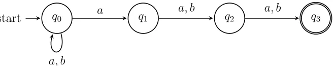
Example 2.3.2. Figure 2.2 shows an NFA M = ({q0, q1, q2, q3},{a, b}, δ, q0,{q3}) which
accepts the language of words overΣ ={a, b}withain the third position from the right, or formally, L3 ={w∈ {a, b}∗ :w=xay, x∈ {a.b}∗, y ∈ {a, b}2}, is shown.
..
q0.
start .... q1 q2 q3
a, b
. a
. a, b
. a, b
Figure 2.2: The NFA M accepting L3
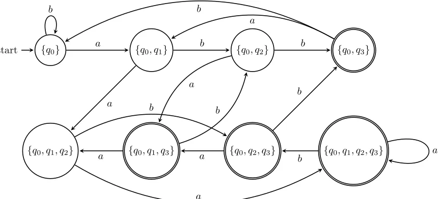
We perform the subset construction to build an equivalent DFAM′ = (Q′,Σ, δ′,{q0}, F′).
The transition functionδ′ is given in Table 2.1. Note that only states that are reachable are listed.
From the transitions given for δ′, we can see that Q′ ⊆ 2Q consists of eight states: {q0},{q0, q1},{q0, q2},{q0, q3},{q0, q1, q2},{q0, q1, q3},{q0, q2, q3}, and {q0, q1, q2, q3}. The
set of accepting states F′ consists of states that contain any of the accepting states in
M. Since F = {q3}, we have F′ ={{q0, q3},{q0, q1, q3},{q0, q2, q3},{q0, q1, q2, q3}}. The
2.3. Finite automata 9
q δ(q, a)
{q0} {q0, q1}
{q0, q1} {q0, q1, q2}
{q0, q2} {q0, q1, q3}
{q0, q3} {q0, q1}
{q0, q1, q2} {q0, q1, q2, q3}
{q0, q1, q3} {q0, q1, q2}
{q0, q2, q3} {q0, q1, q3}
{q0, q1, q2, q3} {q0, q1, q2, q3}
q δ(q, b)
{q0} {q0}
{q0, q1} {q0, q2}
{q0, q2} {q0, q3}
{q0, q3} {q0}
{q0, q1, q2} {q0, q2, q3}
{q0, q1, q3} {q0, q2}
{q0, q2, q3} {q0, q3}
{q0, q1, q2, q3} {q0, q2, q3}
Table 2.1: Table for transition function δ′
..
{q0.}
start .... {q0, q1} {q0, q2} {q0, q3}
{q0, q1, q2}
.
{q0, q1, q3}
.
{q0, q2, q3}
.
{q0, q1, q2, q3}
. a . b . a . b . a . b . a . b . a . b . a . b . a . b . a . b
2.4
Converting regular expressions to finite automata
The following theorem by Kleene [44] establishes the correspondence between regular expressions and finite automata.
Theorem 2.4.1. A language is regular if and only if it is accepted by a finite automaton.
Regular expressions and finite automata are two different tools that we use in differ-ent ways to describe regular languages. We use regular expressions to specify patterns to be matched, while finite automata are used to recognize whether a given input string belongs to a language. As we already mentioned, regular expressions are more convenient for human users to describe regular languages and are easier to write and manipulate than finite automata. On the other hand, finite automata are easier to implement in com-puter programs using structures like switch-case statements or adjacency matrices. The equivalence between languages described by regular expressions and languages accepted by finite automata means that we don’t need to choose between the two.
The first step in implementing regular expressions is to transform the regular expres-sion into an NFA. The simplest method to do this is to construct an automaton known as the position or Glushkov automaton [21, 51]. For a regular expression α, the position automaton has exactly |α|+ 1 states. There are other ways to construct an NFA for a regular expression with fewer states and transitions, such as partial derivative automata or follow automata, but these automata can be derived from the position automaton [9, 36].
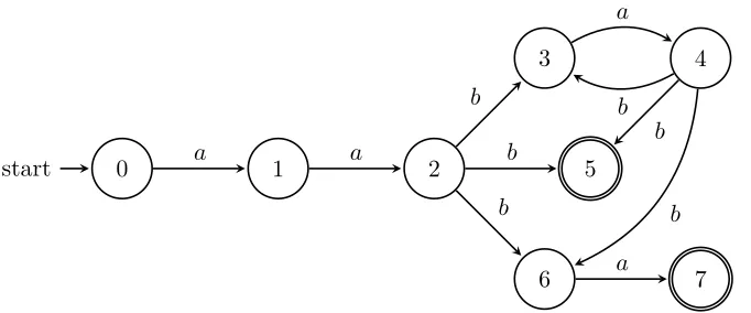
For a regular expression α, let pos(α) ={1,2, ...,|α|}. We mark each letter of α with its position. Let α denote the marked regular expression over Σ = {ai : a ∈ Σ, i ∈ pos(α)}. For example, if α = aa(ba)∗(b+ba), then α =a1a2(b3a4)∗(b5+b6a7). We use
the same notation to remove markings by letting α=α. For ai ∈Σwith i∈pos(α) and
u, v, w ∈Σ∗, we define the following sets:
first(α) = {i:aiw∈L(α)} last(α) = {i:wai ∈L(α)} follow(α, i) = {j :uaiajv ∈L(α)}
The position automaton for α is Npos(α) = (pos(α)∪ {0},Σ, δpos,0,last(α)∪ {0}) with
δpos defined by
δpos(i, a) =
{j ∈follow(α, i) :a =aj} if i̸= 0 {j ∈first(α) :a=aj} if i= 0
2.4. Converting regular expressions to finite automata 11
Example 2.4.1. Letα=aa(ba)∗(b+ba). Thenα=a1a2(b3a4)∗(b5+b6a7)and first(α) =
{1} and last(α) = {5,7}. We define follow(α, i) for 1≤i≤7 in Table 2.2. The position automaton Apos(α) is given in Figure 2.4.
i follow(α, i)
1 {2}
2 {3,5,6}
3 {4}
4 {3,5,6}
5 ∅
6 {7}
7 ∅
Table 2.2: The table for follow(α, i)
.. 0.
start ... 1 2
3
.
4
. 5
.
6 .
7
. a
. a
.
b
. b
.
b
.
a
.
b
.
b
.
b
.
a
Figure 2.4: The position automaton for α=aa(ba)∗(b+ba)
After we construct an NFA, we can transform it into a DFA using the subset con-struction. As we will see shortly, NFAs are much more succinct than DFAs. However, there are some tasks for which DFAs are more well-suited. For instance, membership testing is much more straightforward for a DFA since nondeterminism does not need to be modeled in implementation. Testing for equality is also much simpler since DFAs have a canonical form, the minimal DFA, which we will also introduce shortly.
Note that the DFA that results from the subset construction is not necessarily the minimal equivalent DFA. We would like these DFAs to be as small as possible. This is the problem of DFA minimization. The minimal DFA M for a language L is simply the DFA with the minimal number of states which acceptsL. We have the following property as a result of theorems by Myhill [54] and Nerode [58]:
For an NFA with n states, the number of states in an equivalent DFA can be up to
2n. In other words, a DFA can be exponentially larger than the regular expression that we started out with. This is a problem for implementation because of the memory re-quirements for storing such large structures. While DFAs can be minimized inO(nlogn)
time via Hopcroft’s algorithm [30], this still requires the possibly costly transformation from NFA to DFA.
Chapter 3
The Vertex Cover Problem
3.1
Complexity theory
We measure the time complexity of an algorithm by the number of operations that are performed as a function f(n) of the length n of the input. We say that an algorithm runs in O(g(n))time if there exists a constantc > 0such that for every sufficiently large
n, f(n) ≤ c·g(n). We say that f(n) is o(g(n)) if for every constant c > 0, we have
f(n)< c·g(n) for all sufficiently large n. Similarly, we say that f(n) isΩ(g(n)) if there exists a constant c >0 such that for every sufficiently largen, f(n)≥c·g(n).
A decision problem is a problem which has an answer of either YES or NO. An optimization problem is a problem which attempts to minimize or maximize some value. When discussing the complexity of a problem, we are concerned with decision problems. However, an optimization problem can be easily reformulated as a decision problem which is no harder than the original optimization problem. In other words, the optimization problem can be solved in time that is at most a polynomial factor larger than that for the decision problem.
For instance, given a DFA, the DFA minimization problem asks for an equivalent DFA with the minimal number of states. The answer to the problem is a DFA. We can reformulate the problem as a decision problem by asking whether there exists an equivalent DFA of size at most k, for some integer k. The answer to this problem is either YES or NO. To find a minimal DFA equivalent to a given n-state DFA, we ask whether there is an equivalent DFA of size1,2, ..., n−1, which means asking the decision problem at most n−1 times.
A problem is solvable in polynomial time if there exists an algorithm that solves it in
O(nk) time for constant k. We define P to be the class of decision problems which are solvable in polynomial time. We consider an algorithm to be efficient if it has polynomial
running time and we consider problems to be computationally feasible if they are in solvable in polynomial time.
We define NP to be the class of decision problems that have solutions which can be verified in polynomial time. That is, we can check whether a given solution for an instance of the problem is correct or not in polynomial time. Formally, a verifierV for a problem A is an algorithm that takes as input an instance I of A and a polynomial-size certificateC. V returns YES ifC verifies that the answer to I is YES and NO otherwise.
A can be verified in polynomial time if the time complexity of its verifier is polynomial in the size of I.
A problem is NP-hard if every problem in NP can be reduced in polynomial time to the problem. A problem is NP-complete if the problem is NP-hard and is also in NP. A problem A reduces to a problem B if there is a polynomial-time function f that transforms an instance I of A to an instance f(I) of B such that I is an instance of A
for which the answer is YES if and only if f(I)is an instance of B for which the answer is YES.
By definition, any problem which is in P is clearly in NP, since a problem which is computable in polynomial time will have a solution which is verifiable in polynomial time. Thus, we have the inclusion P ⊆ NP. However, it is currently not known whether P = NP. Since every NP-complete problem reduces to every other NP-complete problem, if there is a polynomial time algorithm for any one NP-complete problem, then there is a time algorithm for every problem in NP. And if there is no polynomial-time algorithm for any problem in NP, then no problem in NP has a polynomial-polynomial-time algorithm. Showing either of these would resolve the P = NP question.
In this thesis, we assume that P ̸= NP and thus, we consider problems which are NP-hard to be intractable.
3.2 The minimal vertex cover problem
A graph G = (V, E) is a pair consisting of a finite nonempty set V of vertices and a collection E of pairs of V, called edges. A hypergraph H = (V, E) is a generalization of a graph and is a pair consisting of a finite nonempty set V of vertices and a collection
E of subsets of V, called hyperedges. H is k-uniform if |e| = k for every hyperedge
3.2. The minimal vertex cover problem 15
... 1 . 2
.
3 .
4 .
5 .
6 .
7
. 8
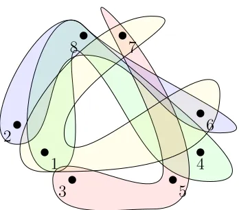
Figure 3.1: The hypergraph H = (V, E)
hypergraph.
A k-colouring of a hypergraph H = (V, E) is a partition (V1, ..., Vk) of V into k colour classes such that each edge contains vertices from at least two colour classes. A hypergraph is k-colourable if it admits ak-colouring. A strong k-colouring is a partition
(V1, ..., Vk) of V such that each edge contains at most one vertex of each colour. A hypergraph is k-strongly-colourable if it admits a strong k-colouring. A hypergraph is
k-partiteif the vertex set can be partitioned intok sets and every hyperedge contains at most one vertex from each partition.
Example 3.2.1. A hypergraph H = (V, E) is drawn in Figure 3.1. H has vertex set
V = {1,2,3,4,5,6,7,8} and hyperedge set E = {{1,6,7},{1,4,8},{2,6,8},{3,5,7}}. The vertices are represented as dots and each hyperedge is represented as a curve. Vertices contained in a curve belong to the hyperedge represented by the curve. Since each hyperedge of H has size exactly 3, H is 3-uniform. We can partition the vertex set of
H into three colour classes: {1,2,3}, {4,5,6}, and {7,8}. Thus, H is also 3-strongly-colourable.
The vertex cover problem is a fundamental combinatorial optimization problem. A vertex cover on a hypergraph H = (V, E) is a subset of vertices C ⊆ V such that every hyperedge in E contains at least one vertex from C. That is, for every e ∈ E(H), we havee∩C ̸=∅. We say a vertex v ∈C covers an edgee ifv ∈e and we say that an edge
e is covered with respect to a cover C if it is covered by a vertex in C. The minimum vertex cover problem is given a hypergraphH= (V, E), find a vertex cover with minimal cardinality. For the weighted version of the problem, a weight functionw:V →Z onH
Example 3.2.2. A vertex cover on the hypergraph H in Figure 3.1 would be the set {4,5,6}; this vertex cover is not the smallest one. The set {7,8} is also a vertex cover for H and is also a minimal vertex cover. We know that a minimal vertex cover has size at least 2, since there is no single vertex which covers all four edges ofH.
The minimum vertex cover problem was one of the first problems shown to be NP-complete by Karp in [40]. For hypergraphs, this problem is equivalent to the set cover problem and we can always reformulate a minimum vertex cover problem on hypergraphs as a minimum set cover problem. The minimum set cover problem asks, for an instance
I = (U, S), where U is the set of ground elements and S ⊆2U is a collection of subsets of U, to find a subcollection C ⊆S such that ∪X∈CX =U of minimal cardinality.
To formulate the instance I as an instance J = (V, E) minimum hypergraph vertex cover problem, we map elements of U to edges in E and subsets fromS to vertices inV. Letf :U∪S →V ∪E by such a map with V ={f(x) :x∈S}and E ={f(x) :x∈U}. Then for x∈U and s ∈S, we have x∈X if and only if f(s)∈f(x).
We are interested in the minimum vertex cover problem for k-uniform k-partite hy-pergraphs. This problem has applications in many areas, among others, NFA reduction, distributed data mining [16] and database schema mapping discovery [22]. When k = 2, or when the graph is bipartite, the problem is solvable in polynomial time, since by König’s theorem, the problem is equivalent to finding a maximum matching. However, for k ≥3, the problem is NP-complete.
Like many combinatorial optimization problems, we can formulate the vertex cover problem as an integer program. The following is the integer program for the vertex cover problem.
minimize ∑
v∈V
w(v)g(v) (3.1)
subject to ∑ v∈e
g(v)≥1,∀e∈E
g(v)∈ {0,1},∀v ∈V
For each vertex v ∈ V, we assign a variable g(v) which takes on a value of 1 if it is in the vertex cover and 0 otherwise. For each edge, at least one of its vertices must be in the vertex cover. This translates into the condition that the sum of the values of the variables for each vertex in an edge must be at least 1. We wish to find a vertex cover with the minimal total weight.
3.3. Approximation Algorithms 17 the condition that variables take on integer values and allow the variables to be real-valued. This is the linear programming relaxation of the integer program. While it may initially seem strange to allow including, say, 1
3 of a vertex in a vertex cover, the linear
programming relaxation has the advantage of being able to be solved in polynomial time. The following linear programming relaxation defines the fractional vertex cover problem.
minimize ∑
v∈V
w(v)g(v) (3.2)
subject to ∑ v∈e
g(v)≥1,∀e∈E
g(v)≥0,∀v ∈V
A feasible solution g for Problem (3.2) is a fractional vertex cover of H. We denote the value of g by |g|=∑v∈V g(v). We define the covering number τ(H) of H to be the size of the minimal vertex cover ofH. Similarly, we letτ∗(H), the fractional covering number of H, denote the minimum value ofg across all fractional covers of H.
We can use the fractional vertex cover to approximate the minimum vertex cover by rounding the valuesg(v)to integer values. The integrality gapof the problem is the ratio of the value of the optimal solution of the linear programming relaxation to the value of the optimal solution for the integer program. For the minimum vertex cover problem, this is the ratio ττ∗((HH)).
3.3
Approximation Algorithms
While finding the optimal solution for many problems is intractable, approximate solu-tions can often be computed efficiently. We can measure the quality of an approximation algorithm by its approximation ratio. Given an optimization problem γ, let the cost or value of an optimal solution for γ be denoted by C∗ and let C denote the value of a solution produced by an approximation algorithm A. Then the approximation ratio of A on input of size n is ρ(n), defined in [10] by
max
{
C C∗,
C∗ C
}
≤ρ(n)
and we say A a ρ-approximation algorithm and we call a solution computed by A a
ρ-approximation.
problem on graphs is a greedy algorithm that selects vertices based on a maximal match-ing, giving a 2-approximation. A matching M of a graphG= (V, E)is a subset of edges such that no two edges in M are adjacent to a common vertex. A maximal matching is a matching M of G such that M is no longer a matching if any edge not in M is added to it. A maximal matching M can be found simply by examining every edge and adding it to M if it is not adjacent to any edge already in M. This can be done in polynomial time.
For a graph G= (V, E), given a maximal matchingM, letCbe the subset of vertices which are adjacent to the edges in M. C is a vertex cover of G, since C covers every edge in E. If there was an edge e∈E that was left uncovered byC, thene would be an edge which could be added to M, contradicting the maximality of M.
Since each edge in M must be covered by one of the vertices it is incident to and the edges of M do not share any vertices, any cover must be at least as large as |M|. Therefore, for any optimal vertex cover C∗,
|M| ≤ |C∗| ≤ |C|= 2|M| ≤2|C∗|.
Thus, this algorithm has an approximation ratio of |C| |C∗| ≤2.
The best approximation algorithm for the minimal vertex cover problem on hyper-graphs achieves an approximation ratio of O(logd), where d is the maximum degree of the hypergraph [49]. When we restrict the size of the edges to at most k vertices, we can apply the same greedy algorithm as in Example 3.3.1 to achieve an approximation ratio ofk. Many algorithms achieve approximation ratios slightly better than this simple
k-approximation.
Lovász gives an upper bound of k
2 for the integrality gap for the minimum vertex
cover problem on k-partite k-uniform hypergraphs [48]. In [1], Aharoni et. al give an example showing that this bound is tight. If we generalize further and consider k-partite
r-uniform hypergraphs (or, equivalently, k-strongly-colourable r-uniform hypergraphs) with r̸=k, Aharoni et. al show an upper bound of
τ(H)
τ∗(H) ≤
k−r+ 1
k r
for k ≥(r−1)r. For r≤k ≤(r−1)r, they show an upper bound of
τ(H)
τ∗(H) ≤
kr
k+r +min
{
k−r
2k {u}, r
k(1− {u})
}
3.3. Approximation Algorithms 19 where u = k2
k+r and {u} =u− ⌊u⌋. If we consider k-colourable r-uniform hypergraphs, Krivelevich [46] shows an upper bound of max{k+1
k r, r−1
}
and gives two algorithms that compute approximate solutions that achieve the above approximation ratio.
A natural question to ask is whether we can approximate the optimal solution of a problem to within an arbitrary factor in polynomial time. Solving a problem exactly may be difficult, but if we can compute a solution that is within, say, 1% of an optimal solution, in many cases, we would be quite pleased with the result. For some problems, like the knapsack problem [31], it is possible to design an ρ-approximation algorithm for everyρ >1.
However, it has been shown that problems like minimum set cover and minimum vertex cover cannot be ρ-approximated for every ρ > 1. A problem is said to be inap-proximable to within a factor ofρif there is noρ-approximation algorithm for it that runs in polynomial time, unless P = NP. If such an algorithm existed, then it would imply that P = NP. This means that for the set cover and vertex cover problems, there is a limit to how good approximate solutions can be computed in polynomial time, assuming P ̸=NP.
Arora showed an integrality gap of 2−ϵ, for some small ϵ >0, for the vertex cover problem on graphs [4], which matches the best known approximation ratio for algorithms based on a linear programming relaxation of the problem; Håstad [26] showed that the problem is inapproximable to within a factor of 7
6 −ϵ, for certain small ϵ >0, and Dinur
and Safra improved this bound to 1.36 [15].
For general hypergraphs with unbounded edge size, the problem is inapproximable to within a factor of (1−o(1))lnn, where n is the number of hyperedges [17]. A num-ber of inapproximability results were shown by using the PCP theorem, which relates proof checking with approximability [42]. The earliest inapproximability result for k -uniform hypergraphs was presented by Trevisan in [66] showing inapproximability to within Ω(k191 ). Holmerin improved this to Ω(k1−ϵ) in [28]. Dinur et. al show inapprox-imability to within k−3−ϵ in [13] shortly before improving the result to k−1−ϵ in [14].
In [1], Aharoni et. al constructed an instance which matched the k
2 upper bound on
the integrality gap given by Lovász. A recent result by Guruswami and Saket [25] shows that vertex cover onk-partitek-uniform hypergraphs is inapproximable to within a factor of k
4 −ϵ fork ≥16. This result is based on a reduction from k-uniform hypergraphs and
uses the inapproximability result from [14]. The result is improved further by Sachdeva and Saket [64] to k
2 −1 + 1
Improved inapproximability results can be achieved using the Unique Games Con-jecture of Khot [41]. The UGC provides a convenient reduction for certain classes of problems for which using the PCP theorem may be challenging. Assuming that the UGC holds, Khot and Regev [43] show inapproximability of vertex cover on graphs within a factor of2−ϵ. They also show inapproximability withink−ϵfork-uniform hypergraphs under this assumption. In [25], Guruswami and Saket also include a UGC-based inap-proximability result of k
2 −ϵ for k-uniform k-partite hypergraphs. This result matches
Chapter 4
The NFA reduction problem
4.1
Preliminaries
While DFA minimization is computable in polynomial time, NFA minimization is known to be PSPACE-complete [37] and, therefore, is much more computationally difficult, assuming P ̸= PSPACE. PSPACE is the class of problems which can be solved with a polynomial amount of space and a problemAis PSPACE-complete if every other problem in PSPACE can be reduced into A in polynomial time. This means that if a PSPACE-complete problem could be solved in polynomial time, then all problems in PSPACE could also be solved in polynomial time. While it is clear that P ⊆ NP ⊆ PSPACE, it is not known whether P = PSPACE. Not only is the problem extremely difficult, but even approximating it is hard. Given ann-state NFA, computing an equivalent minimal NFA is inapproximable to within a factor of o(n) unless P = PSPACE [23]. This means that any polynomial time algorithm that reduces the size of an NFA cannot give any guarantees on the size of the reduction that is sub-linear in the size of the given NFA unless P = PSPACE.
Because of the computational hardness of the problem, there have been a variety of approaches to try to make the problem feasible. There are exact minimization algorithms from Kameda and Weiner [38] and Melnikov [52] which are infeasible in practice. Ilie and Yu introduce a method which involves merging states based on equivalence relations [35]. Champarnaud and Coulon extend that idea by using preorder relations [8]. Geldenhuys, van der Merwe, and van Zijl propose a technique which transforms instances of NFA reduction into instances of SAT and using SAT solvers to compute reduced NFAs [20].
While NFA minimization is hard in general, a natural question is whether there are any families of languages or restrictions on automata for which the problem is feasible. Gruber and Holzer study the problem restricted to unary and finite languages [24]. They
find that given an n-state DFA which accepts a finite language, finding an equivalent minimal NFA is DP-hard. DP is the class of problems which are the intersection of a problem in NP and a problem in co-NP, where co-NP is the class of problems whose complements are in NP [61]. For unary languages, if an n-state DFA is given, the problem has an O(√n)-approximation, while the problem remains inapproximable to within a factor of o(n) given an n-state NFA, unless P = NP.
Gramlich and Schnitger show in [23] that, given an n-state DFA, finding an equiva-lent minimal NFA is inapproximable to within a factor of √n
poly(logn). They also show that
for an n-state NFA accepting a unary language, finding an equivalent minimal NFA is inapproximable to within a factor of n1−δ for all δ > 0. In [5], Björklund and Martens attempt to resolve a question posed by Malcher in [50], which asks whether there are any useful extensions of DFAs with limited amounts of nondeterminism for which mini-mization is tractable. They find that forδNFAs, a class of NFAs which have at most two computations for every input string, minimization remains NP-hard.
We base our work on research done by Ilie, Solis-Oba, and Yu in [34]. In the paper, the authors show how to compute optimal reductions by merging states based on the equivalences introduced in [35] and the preorders from [8]. To help define various language relations over states of NFAs, we give the following definitions. The language recognized by an NFA N = (Q,Σ, δ, q0, F) is L(N) = {w ∈ Σ∗ : δ(q0, w)∩F ̸= ∅}. For states
p, q ∈Q, we define
LL(N, p) ={w∈Σ∗ :p∈δ(q0, w)}
LR(N, p) ={w∈Σ∗ :δ(p, w)∩F ̸=∅} L(N, p, q) ={w∈Σ∗ :q∈δ(p, w)}
For simplicity, we write LL(p), LR(p), and L(p, q), respectively when N is understood.
4.1.1 Reducing NFAs based on equivalences
In [35], Ilie and Yu define equivalence relations on the states of an NFA. An equivalence relation on a setS is a relation≡ ⊆S×S which satisfies the following for alla, b, c∈S:
• Reflexivity: a≡a
• Symmetry: if a≡b, thenb ≡a
4.1. Preliminaries 23 An equivalence relation partitions the setS into equivalence classes. Two elements a, b∈ S belong to the same equivalence class X if and only if a ≡ b. For a subset T ⊆ S,
T/≡ denotes the quotient set {[a]≡ : a ∈ T}, where [a]≡ denotes the equivalence class containing a. Let ≡ and ∼= be two equivalence relations over the set S. We say that ∼=
is coarser than ≡ if a≡b implies a∼=b.
An equivalence relation≡isright-invariantwith respect to an NFAN = (Q,Σ, δ, q0, F)
if it satisfies the following:
1. ≡ ⊆(Q\F)2∪F2
2. for every p, q ∈Q, a∈Σ, ifp≡q, then δ(p, a)/≡ =δ(q, a)/≡
For an NFA N = (Q,Σ, δ, q0, F), the equivalence relation ≡R is defined to be the coarsest right-invariant equivalence relation on a state set Q that satisfies the following:
(P1) ≡R∩(F ×(Q−F)) =∅
(P2) ∀p, q ∈Q,∀a ∈Σ,(p≡Rq=⇒ ∀q′ ∈δ(q, a),∃p′ ∈δ(p, a), q′ ≡R p′)
The left equivalence≡Lis defined to satisfy the same axioms on the reversed automaton, which is constructed by reversing the transitions of N and exchanging the initial and final states. Ilie, Navarro, and Yu show in [32] that equivalences over the state set can be computed using a partition refinement algorithm by Tarjan and Paige [60] with
O(mlogn) time and O(m +n) space, where n is the number of states and m is the number of transitions.
Each equivalence class of≡R and≡L represents equivalent states that can be merged into a single state without modifying L(N). We merge a state p with a state q by replacing all incoming and outgoing transitions of p with q and deleting p. Since ≡R is right-invariant, it has the property that for some word w =a1a2· · ·an ∈ LR(p), there is a path pa1p1a2p2· · ·anpn in N with pn ∈ F such that there exists a path qa1q1· · ·anqn inN with pi ≡R qi for all 1≤i≤n and qn ∈F. This implies that w∈ LR(q) and, thus, merging p and q does not change L(N). The same reasoning applies for ≡L.
vertex cover problem on bipartite graphs, which can be solved in polynomial time [34]. We call the resulting optimally reduced NFA an eq-reduced NFA. We note that this is not a minimal NFA.
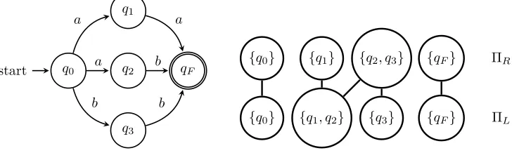
Example 4.1.1. Let N = (Q,Σ, δ, q0, F) be as in Figure 4.1. The equivalence classes
for ≡R are {q0}, {q1}, {q2, q3}, and {qF} and the equivalence classes for ≡L are {q0},
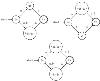
{q1, q2}, {q3}, and {qF}. The instance of vertex cover constructed from the partitions of the equivalences is also shown in Figure 4.1. The vertices are subsets of the state set which are equivalent, either under ΠR or ΠL. Each edge represents a state and is incident to the vertices which represent the subset which contains the state. Based on this instance, there are three possible eq-reduced automata for N, which are given in Figure 4.2.
..
q0.
start .. q2
q1
.
q3
. qF
.
a
. a .
b
.
a
. b
.
b
..
{q....0} {q1} {q2, q3} {qF}
{q0}
.
{q1, q2}
.
{q3}
.
{qF}
.
ΠL
. ΠR
...
Figure 4.1: The NFA N and the set cover instance (Q,ΠR∪ΠL)
4.1.2
Reducing NFAs based on preorders
In [8], Champarnaud and Coulon extend the idea of merging equivalent states by using preorder relations defined on the states of an NFA. A preorder on a set S is a relation ≤ ⊂S×S which satisfies the following for all a, b∈S:
• Reflexivity: a≤a
• Transitivity: ifa ≤b and b≤c, then a≤c
A partial order is a preorder which is alsoantisymmetric: ifa≤b andb ≤a, then a=b. If the preorder is symmetric, then by definition, it is an equivalence relation. A partially ordered set, or poset, is a pair consisting of a set and a partial order over the set.
The preorders are defined as follows.
p≤Rq if LR(p)⊆ LR(q)
4.1. Preliminaries 25
..
q0.
start .
q1
.
{q2, q3}
. qF
. a . a, b . a .
b start q..0..
{q1, q2}
.
q3
. qF
. a . b . a, b . b ..
q0.
start .
{q1, q2}
.
{q2, q3}
. qF
. a . a, b . a, b . b
Figure 4.2: eq-reduced NFAs for the NFA N
Ilie, Navarro, and Yu give an algorithm in [32] which computes preorders over the state set inO(mn)time andO(n2)space, wheren is the number of states andmis the number of transitions.
These preorders induce equivalence relations that are coarser than the equivalence relations defined above. Specifically, we define the equivalence relation∼=R if p≤R q and
q ≤R p and ∼=L if p ≤L q and q ≤L p. These equivalence relations induce a partition of the state set. We denote by πL and πR the partitions of the state set induced by the equivalences ∼=L and ∼=R respectively. The preorders also induce a partial order ⪯ on the state set: p ⪯ q iff p ≤R q, p ≤L q, and L(p, p) = {ϵ}. The partial order ⪯ induces a familyπP of subsets ofQ: let the maximal elements of⪯beq˜1,q˜2, ...,q˜m. Then
πP ={Qp1, ..., Qpm}, where Qpi ={q ∈Q:q ⪯q˜i}.
a pre-reduced NFA.
Example 4.1.2. The following example is used by Champarnaud and Coulon [8] to demonstrate how preorders can capture a wider range of equivalent states than the equivalences defined in [35]. Let N = (Q,Σ, δ, q0, F) be as depicted in Figure 4.4. The
preorders on Qare as follows:
≤R={(q1, q2),(q2, q1),(q3, q4),(q5, q4)}
≤L={(q3, q4),(q5, q4)}
These preorders give rise to the following equivalence classes for∼=Rand∼=L, respectively:
πR ={{q0},{q1, q2},{q3},{q4},{q5},{qF}}
πL ={{q0},{q1},{q2},{q3},{q4},{q5},{qF}}
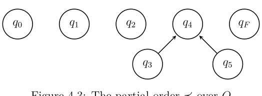
The preorders also induce the partial order ⪯, which is given in Figure 4.3 and induces the following family of subsets:
πP ={{q0},{q1},{q2},{q3, q4, q5},{qF}}
..
q....0 q1 q2 q4
q3
.
q5
. qF
..
Figure 4.3: The partial order ⪯ over Q
Note that we have q1 ∼=R q2, since q1 ≤R q2 and q2 ≤R q1. This equivalence would
not have been included in ≡R, since there are no states that are equivalent for q3 or q5
under ≡R. We also have q3, q5 ⪯q4, which is another relation that would not have been
captured by ≡R and ≡L.
From the hypergraph of the set cover instance (Q, πR∪πL∪πP) in Figure 4.5, we can see a vertex cover{{q0},{q1, q2},{q3, q4, q5},{qF}}. The pre-reduced NFA is shown in Figure 4.6.
4.1. Preliminaries 27
..
q0.
start . q1 . q2 . q3
. q4
.
q5
. qF
. a . b . a . a . a . a . a
. a, b
.
b
Figure 4.4: The NFA N
...
πL .
πR
.
πP
. {q0}
.
{q1, q2}
.
{q3}
.
{q4}
.
{q5}
.
{qF}
. {q0}
.
{q1}
.
{q2}
.
{q3}
.
{q4}
.
{q5}
.
{qF} .
{q0}
.
{q1}
.
{q2}
.
{q3, q4, q5}
.
{qF}
Figure 4.5: The hypergraph for the set cover instance (Q, πR∪πL∪πP)
..
q0.
start .... {q1, q2} {q3, q4, q5} qF a, b
. a
. a, b
Example 4.1.3. In Figure 4.7, there are two equivalent NFAs which accept the language {a, b}2. The NFA on the right is the pre-reduced automaton derived from the NFA on
the left, since q1 ⪯q2.
..
q0.
start .
q1
.
q2
. qF
.
a
.
a
.
a, b
.
a, b
..
q0.
start ... q2 qF a, b
. a, b
Figure 4.7: NFAs which accept the language {a, b}2
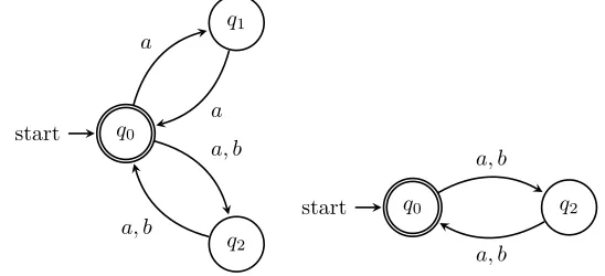
Suppose we use the NFAs from Figure 4.7 to construct NFAs which accept ({a, b}2)∗.
The pre-reduced NFAs derived from those automata are given in Figure 4.8. The au-tomaton on the left is unable to be reduced further because although q1 ≤R q2 and
q1 ≤Lq2, we have L(q2, q2)̸={ϵ}.
..
q0.
start .
q1
.
q2
.
a
. a
.
a, b
.
a, b
..
q0.
start .. q2
a, b
.
a, b
Figure 4.8: NFAs which accept the language ({a, b}2)∗
4.2
Complexity of computing
pre
-reduced NFAs
4.2. Complexity of computing pre-reduced NFAs 29 be 3-uniform and can possibly have a worst-case approximation ratio of O(logd), where
d is the size of the largest edge. However, there are families of languages for which the
pre-reduced NFAs that recognize them can be computed in polynomial time. We now give several examples of such families. First, we have the following lemma.
Lemma 4.2.1. Let N be an NFA. Suppose every state of N belongs to a cycle. Then N
can be pre-reduced in polynomial time.
Proof. Let N = (Q,Σ, δ, q0, F). Consider a state p ∈ Q. Since p belongs to a cycle,
L(p, p) ̸= {ϵ}. Thus, there is no state q ∈ Q such that p ⪯ q. This means that πP consists of singletons and thus it does not contribute any candidate states to be merged when pre-reducing N. All possible state merges occur in πL and πR, so the problem of computing the pre-reduced NFA for N can be reduced to the minimum vertex cover problem on a bipartite graph [34].
Brzozowski and Cohen define a regular star language in [6] to be a language L⊆Σ∗
such that L=R∗ for some regular languageR ⊆Σ∗.
Lemma 4.2.2. Let L = R∗ ⊆ Σ∗ be a regular star language. Then given a trim NFA
N(R) accepting R, a pre-reduced NFA accepting L = R∗ can be computed in time polynomial in the number of states and transitions of N(R).
Proof. LetN(R) = (Q,Σ, δ, q0, F) denote an NFA accepting R. Recall that a trim NFA
is an NFA with no unreachable or dead states. We follow the construction from [29] to construct an NFA N(R∗)which accepts R∗. There are two cases to consider.
The first case is if ϵ∈R. Let N(R∗) = (Q,Σ, δ′, q0, F). Then we define δ′ as follows.
For every q∈Q and everya ∈Σ,
δ′(q, a) =
δ(q, a) if q̸∈F δ(q, a)∪δ(q0, a) if q∈F
Now consider all states q ̸= q0 in Q. Since each of these states has a path to a final
state and all states are reachable from q0, then every state q ̸= q0 has a path to itself.
Therefore, each of these states belongs to a cycle. If q0 is also contained in a cycle, then
by Lemma 4.2.1, this NFA can be pre-reduced in polynomial time.
If q0 is not contained in a cycle, observe that LL(q0) = {ϵ}. Since q0 is the initial