Development of Experimental Data Based Model Using DA
Technique with ANN for I.C. Engine Operating Performance
Analysis
Dr. M.S. Deshmukh1,Dr. D.S. Deshmukh2, Dr. M. R. Phate3
1,3
Associate Professor, AISSMS College of Engineering, 1-Kennedy Road, Near RTO Square, Pune (M. S.) India 1,
[email protected] (m) – 9922946761, [email protected], (m)-7058816968 2
Associate Professor, G H Raisoni College of Engineering. Near CRPF Campus, Hingna Road, Nagpur (M. S.) India 2
[email protected] (m) – 9822418116
Abstract :Operating performance of an Internal Combustion engine is especially important from the environmental pollution problems point of view. Design considerations for any machine are having common objectives, to obtain highest possible efficiency and another is to obtain minimum possible environmental degradation. Compression Ignition engine consist of load on engine, engine speed, backpressure on engine and fuel consumption as main operating variables.
Dimensional analysis technique is employed for reduction of variables. The Backpressure acting on engine is most important factor which basically deteriorates the engine and emission control performance. In the present work, Modeling is done for determining the relationship between operating variables of Internal Combustion engines. Backpressure is generated on a C.I. engine, with and without the use of a specially designed Diesel Particulate Filter for modeling purpose. Using the theories of engineering experimentation design of experiments followed by testing is done. Correlation coefficient between observed data and computed data from the mathematical model is determined. The Backpressure acting on engine is most important controllable operating parameter of engine. The present work Shows vital scope for improvement of operating performance of engine by optimization of the model formed, in case of each type of I.C. engine.
Keywords- 4S CI Engine, Dependent Variables, Independent Variables, DPF, DA Modeling, ANN
1. INTRODUCTION
The theory of experimentation as suggested by Hilbert [1] is a good approach of representing the response for this task of I.C. engine operating performance improvement in terms of proper interaction of various inputs of the phenomenon. In fact, it‟s felt that such an approach isn‟t yet seen towards analysis on I.C. engines. This approach finally establishes associate experimental data-based model for any phenomenon. It is felt in this investigation to adopt this approach for formulating the model correlating various inputs to a phenomenon of engine operation [1].
In this complete process, three crucial steps viz. Planning, Operation and Data analysis, are adopted. In experimental designing step, study of instruments to be used for precision and accuracy errors is done. Due thought is given like plan for replication of readings against constant inputs for better accuracy. Then estimation for the form of experimental function which governs the task is done, using the known or estimated precision-error data and the methods to predict the propagation of error during the test. If the error analysis does not show the test to be too imprecise, examination of the independent and dependent variables, using dimensional analysis, for possible reduction in their number is carried out. It is decided, how the selected independent variables are to be spaced and what sequence will be followed in setting each point in turn. In this experimentation conventional plan of experimentation is followed.
By fixing the location at Nagpur, India for experimentation due care is taken for extraneous variables. In the step of Operation, it is necessary to evolve physical design of an experimental set up having provision of setting test points, adjusting test sequence, executing
proposed experimental plan, provision for necessary experimentation for noting down the responses is done. Experimental set up is arranged as there is not much scope for design except putting engine systems together. The range for independent variables is selected properly within the test envelope as proposed in the experimental plan. In the field of experimentation, we have to carry out the experimentation using the available ranges of the various independent variables to assess the value of the dependent variable.
Sufficient data have been collected and this data is converted in the usable form for analysis purpose by observing complete data sets for one or more wild points or outliers, so that it may be rejected by providing a reasonable criterion viz. by varying on variable at a time is followed. In this final step of data analysis, qualitative as well as quantitative approach is used to achieve the task of modeling for the phenomenon [2].
2. REDUCTION OF VARIABLES:
This is achieved by applying Buckingham‟s pi theorem (Hilbert, 1961). When we apply this theorem to a system involving n independent variables, (n minus number of primary dimensions viz. L, M, T, Ө) viz. (n - 4) numbers of pi terms are formed. When n is large, even by applying this theorem number of pi terms will not be reduced significantly than number of all independent variables. In this work to obtain different solutions for each type of internal combustion engine performance improvement almost all the possible variables are considered for experimental data-based modeling of operating variables for determination of dimensionally homogeneous equations [1,3]. Brief summary of variables is given here.
Input Variables :
1) Heat Input : It is dependent on mass flow rate of fuel and air and also on the fuel properties specially Calorific value of fuel.
2) Compression ratio : It is the ratio of total cylinder volume to clearance volume, depends upon cylinder dimensions such as Stroke length, Crank radius, Cylinder/piston Diameter and clearance space.
3) Load on engine : Load factor on engine is an independent variable, as per the total load requirements such as vehicle weight, weight of passengers, road resistance or slope condition, drag force variations, electrical load etc. which is based upon the traffic environment in which the engine operates, state of maintenance and repair which is not easily measured in terms of energy consumption also driver‟s skill is very important parameter since use of gear, clutch and brake are very crucial aspects of engine out performance.
4) Pressure of air at the inlet and outlet to engine cylinder : It is dependent on the design of inlet and outlet manifold systems used, Atmospheric pressure and temperature also.
5) Engine Speed : As per the time availability or torque requirements, engine speed is altered or decided.
Output Variables or Response Variables :
1) Brake Power : It is the power available at the output shaft. It is dependent on engine speed and load on engine. Engine speed is also an independent variable, as per the availability of time or time requirements; speed can be kept constant as in case of diesel generator applications with the help of a governor. Speed can be increased or decreased using accelerator or gear box mechanisms. At constant brake power these values of speed and load are varied using gear box arrangement as per engines operating needs, for example during starting a vehicle speed is kept low but high torque is supplied to the wheels. Frictional power loss variation is also depending on load and speed variations.
2) Operating parameters of engine: Cylinder pressure variation with respect to crank rotation/angle, Cylinder liner temperature, Exhaust gas parameters at outlet such as mass flow rate of exhaust gases, Composition of exhaust gases or exhaust emissions (i.e. HC, CO, NOx, PM etc.), pressure of exhaust gases just at engine cylinder outlet.
3) Heat balance sheet: Heat equivalent of brake power, Heat carried away by cooling water, Heat carried away by exhaust gases, Heat unaccounted [3,4,5].
Applying Buckingham‟s pi theorem, the different equations are obtained but after critical study of different π
terms it is decided to proceed with only operating variables for a specific C.I. engine under consideration. Engine performance is basically dependent on fuel consumption, which bears direct influence on efficiency and engine out emissions. So, fuel consumption rate is a basic dependent variable, It is an important parameter of an engine, varies because of any possible variable variations such as engine design, its operating conditions, fuel composition and After treatment system or exhaust system utilized. Backpressure on engine is defined as pressure exerted in backward direction of the piston motion during exhaust stroke. The backpressure acting on engine is most important and controllable engine operating variable which basically deteriorates the engine and emission control performance. Future modifications should be drained such the simplest way that every alternation mustn't cause backpressure rise. Carefulanalysisof
application surroundings and additional stress is needed, for the fulfillment of sturdiness necessities, chiefly on catalyst reactivation or replacement techniques development.
Further chemical limits on fuel oil Sulphur, phosphorus and sulphated ash are required to be tightened for the protection of aftertreatment devices. Key factor for achieving the objective of economical maximum conversion efficiency of the pollutants with waste energy recovery without adversely affecting the engine performance and also with durability issues is minimum possible backpressure [6,11,12].
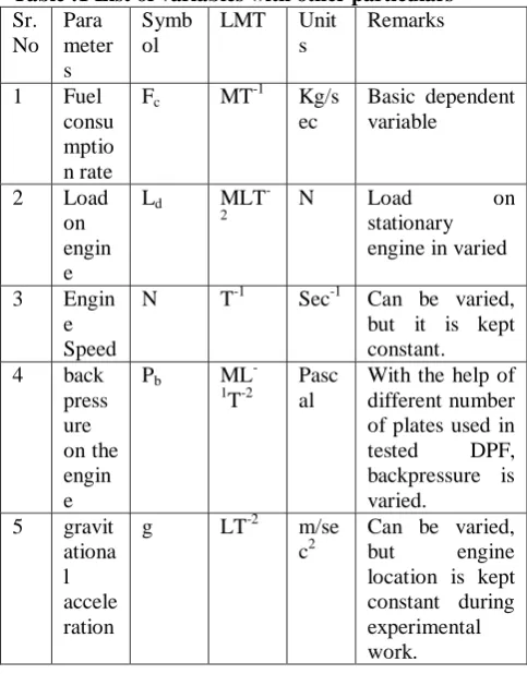
Finally, in this analysis the fuel consumption (Fc) of four strokes, single cylinder C.I. engine during a test run is considered as dependent upon load(ld), speed(N), back pressure (Pb) on the engine and gravitational acceleration (g). Using Buckingham`s л –theorem [13,14]. List of variables with other particulars are given in Appendix table :1.
The fuel consumption (Fc) depends upon (i) ld, (ii) N (iii)
Pb and (iv) g, hence Fc is a function of ld, N, Pb and g.
Mathematically, Fc = f ( ld, N, Pb, g) -(I)
Or it can be written as ƒ(Fc, ld, N, Pb, g) = 0 -(II)
Therefore, total no of variables, n = 5, No of fundamental dimensions, m = 3
( m is obtained by writing dimensions of each variables as Fc = MT-1, ld = MLT
-2
,
N=T-1, Pb =ML-1 T-2 & g = LT-2. Thus, the fundamental dimensions in the problems are M, L, and T hence m = 3). Therefore, the number of dimensionless л - terms = n - m = 5 – 3 = 2
Thus, two л - terms, say л1, л2 are formed. Hence equation
(II) is written as
ƒ(.л1, л2) = 0 ---(III)
Here m is equal to 3 and also called repeating variables. Out of five variables Fc, ld, N, Pb and g, three variables are
to be selected as repeating variables, Fc is a dependent
variable and should not be selected as repeating variables. Out of 4 remaining variables. The variables ld, N, and Pb
are selected as repeating variables. The variables themselves should not form a dimensionless term and should have themselves fundamental dimensions equal to m = 3 here. Dimensions of ld, N, and Pb are MLT
-2
ld, N, and Pb and also, they themselves do not form
dimensionless group.
Each л - term is written as according to the equation л1 = lda1 Nb1 Pbc1. Fc
л2 = lda2 Nb2 Pbc2. g……… …. (IV)
Each л - term is solved by the principle of dimensional homogeneity.
For the л - term, we have л1 = Mo.Lo.To
= (MLT-2)a1 (T-1)b1 (ML-1T
-2
)c1 MT-1
Equating the powers of M, L and T on both sides, we get Power of M, 0 = a1 +c1+1, a1 +c1 = -1
--- (i) Power of L, 0 = a1-c1
--- --(ii) Subtracting equation (ii) from (i),
c1 = -1/2 and by putting this value in equation (i), a1 = -1/2
Power of T, 0 = -2 a1 –b1 -2 c1 -1, -1 = 2 a1 +b1
+2 c1 ---(iii)
Putting values of a1 & c1, we get, 2 (-1/2) + b1+2 (-1/2)
= -1
-1+b1 -1 = -1, b1 = -1 + 2 = 1
---(iv)
Substituting the values of a1, b1, and c1 in equation (IV),
л1= ld -1/2.N1.Pb-1/2.Fc
l
p
b d 1.
.Fc
N
л2 = ld a2
Nb2 Pb c2
.g
= Mo Lo To = (MLT-2)a2 (T-1)b2 (ML-1 T-2)c2 LT-2 Equating the powers of M, L, and T on both sides, we get Power of L, 0 = a2 + c2
Power of M, 0 = a2 - c2 +1, c2= 1/2, , a2 = -1/2
Power of T, 0 = - 2a2 – b2 - 2c2 , 0 = 1 - b2 -1, b2 = 0
Substituting the values of a2, b2 and c2 in equation (IV),
л2 = ld -1/2
N0 Pb 1/2
.g
d b
L
P
g
2Substituting the value of л- terms in equation (III), ƒ(.л1,л2) = 0
ƒ
d b
l
P
g
,
.
.Fc
N
l
p
b d= 0, or
l
p
b.
d.Fc
N
= ƒ
d b
l
P
g
3. EXPERIMENTATION
Single cylinder, four stroke Compression Ignition engine and Tested Diesel Particulate Filter are selected for the experimental task. In the present work, throughout the complete trials conducted, engine jacket cooling water and speed is kept constant at 0.1666 liters/sec and 1500 rpm respectively, so as to provide ease in comparison of different parameters. Perforated circular copper plates arrangement in Diesel Particulate Filter is used as a test
piece for back pressure variations. In some cases, load on engine is also varied in 5 steps. Further during the trials on DPF, each times the fresh perforated plates and rings are used. The different parameters are kept at the planned level with the help of Tested DPF, for the different engine output conditions [9,11,12].
An approach to vary independent л- term, experimental plan is executed, minimum 05 numbers of load variations are achieved keeping all other parameters constant and also minimum 05 numbers of Backpressure variations are achieved keeping all other parameters constant to obtain different power output conditions. Thus, minimum total 10 numbers of fuel consumption rates as response observations are obtained keeping the all other parameters constant. During the trials, 25 trials are conducted and distinct observations are obtained. Out of 25 readings only selected10 test readings that satisfy the criteria of only one variation of variable at a time, are used for analysis. The data of the independent and dependent parameters of the system has been gathered during the experimentation. Causes of errors or the deviations in tests may be a result of the lack of control in holding the variables at their planned levels, or simple lack of precision in the measurements [1].
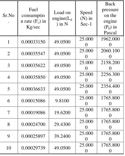
Each observation is taken when the engine setup reaches at steady state condition to minimize error. The observations recorded after performing the measurement of performance parameters of the C.I. engine, then the conversion of observed data in to usable form. See Appendix table :2 and Calculations for model formulation are shown in Table :3.
Engine specifications:
1. Make: Kirloskar, single cylinder, four stroke Compression Ignition engine
2. Rated power output: 5 H.P 3. Stroke length: 110 mm 4. Bore diameter: 80mm
5. Loading type: Water resistance type load, with copper element and load changing arrangement
6. Moment arm: 0.2 meter
7. Orifice diameter (for air box): 25mm 8. Co-efficient of discharge of orifice: 0.64 Tested Diesel Particulate Filter specifications: 1) Space velocity: 50,000 hr-1
2) Catalyst used: copper-based catalyst system
3) Circular perforated copper plates with 256 numbers of holes per square cm and copper rings made up of 5 mm diameter rod.
4) Flange arrangement for dismantling and varying no. of perforated plates and no. of rings (see Appendix figure: 1).
4. DEVELOPMENT OF EXPERIMENTAL DATA
BASED MODEL
One independent pi term (viz. π2) and one dependent pi
term (viz. π1) have been identified in the design of
This correlation is nothing but a mathematical model as a design tool for engine system performance analysis. The optimum values of the independent pi terms can be further decided for optimization of this model for maximum efficiency with due considerations for the constraints in each engine application.
Development of model for dependent pi term π1
We have, π1 = f (π2)
where „f‟ stands for “function of”.
A probable exact mathematical form for this phenomenon could be
π1 =K1*(π2)a1 1.1
There are two unknown terms in the equation 1.1, viz. constant of proportionality K1 and indices a1. To get the
values of these unknowns we need minimum two sets of values of π2. As per the experimental plan in design of
experimentation we have 05 sets of these values as given in Table :2. If any arbitrary one set from this table is selected and the values of unknowns K1and a1 are
computed, then it may not result in one best unique solution representing a best-fit unique curve for the remaining set of the values. To be very specific we can find out nCr combinations of r sets taken together out of
the available n sets of the values. The value nCr in this case
will be 10. Solving these many sets and finding their solutions will be a Herculean task. Hence, it was decided to solve this problem by curve fitting technique (Spiegel 1980). To follow this method, it is necessary to have the equations in the form as under.
Z = a + b * x + c * y +d * z +… 1.2 The equation 1.1 can be brought in the form of equation 1.2 by taking the log of both sides. By taking the log of both the sides of this equation we get,
log π1 = logK1 + a1 * log (π2) 1.3
Let, log π1 = Z1, logK1 = K1‟, log (π2) = A,
Then the equation 1.3 can be written as
Z1 = K1‟ + a1*A 1.4
Equation 1.4 is a regression equation of Z on A, In an n-dimensional co-ordinate system this represents a regression hyper-plane. To determine the regression hyper- plane, we determine a1 in equation 1.4 so that
Z1 = nK1‟ + a1 *A
Z1*A= K1 ‟A + a1 *A*A
1.5
Where, n is the number of runs or the number of sets of the values.
These equations are called normal equations corresponding to the equation 1.4 and are obtained as per the definition. In the above sets of equation, the values of the multipliers of K1‟and a1 are substituted to compute the
values of the unknowns (viz. K1‟and a1). The values of the
terms on L.H.S. and the multipliers of K1‟and a1 in the sets
of equation 1.5 are calculated. After substituting these values in the equation 1.5 we will get one set of equation which are to be solved simultaneously to get the values of K1‟and a1.
The matrix method of solving these equations using „MATLAB‟ is given below.
Let, A = 2x2 matrix of the multipliers of K1‟and a1.
B = 2x1 matrix of the terms on L.H.S. and
C = 2x1 matrix of solutions or values of K1‟and a1.
Then, C=INV (A)*B 1.6
It gives the unique values of K1‟= 0 and a1= - 2.3710, from
K1‟we have determined value of K1 = 1.000000
Therefore, Model of experimental data based modeling for I.C. engine operating performance analysis would be π1 = 1.00000 *(π2)-2.3710
Observed values and computed values with the help of this model formed is shown in Appendix (Table :4)
5. COMPUTATION OF THE PREDICTED
VALUES BY ANN
One of the most problems in analysis is prediction of future results. The experimental data-based modeling achieved this through mathematical model for the dependent pi term. In such complex phenomenon involving non-linear systems it is also planned to develop using artificial neural network (ANN). The output of this network is often evaluated by examination it with ascertained information and also the information calculated from the mathematical models. For development of ANN the designer must acknowledge the inherent patterns. Once this can be accomplished coaching the network is usually a fine-tuning method.
An ANN consists of 3 layers of nodes viz. the input layer, the hidden layer or layers (representing the synapses) and the output layer. It uses nodes to represent the brains neurons and these layers are connected to each other in layers of processing. The specific mapping performed by ANN depends on its design and values of conjugation weights between the neurons. ANN, as such is highly distributed representation and transformation that operate in parallel and has distributed control through many highly interconnected nodes. ANN were developed utilizing this black box concepts.
Procedure for Model Formulation in ANN: Totally different software/tools have been developed to construct ANN. MATLAB being internationally accepted tool, has been selected for developing the ANN for the complex phenomenon. The various step followed in the developing algorithm to form ANN are as given below.
i) The observed data from the experimentation is separated into two parts viz. input data or the info of independent pi terms and also the output data or the information of dependent pi terms. The input data and output data are stored in test.txt and target.txt files respectively.
ii) The input and output data is then read by the using the DLMREAD function.
iii) In preprocessing step, the input and output data is normalized.
iv) Through principle component analysis the normalized data is uncorrelated. This is achieved by using prepca function. The input and output data are then categorized in three categories viz. testing, validation and training. The common practice is to select initial 75% data for testing, last 75% data for validation and middle overlapping 50% data for training. This is achieved by developing a proper code.
v) The data is then stored in structures for testing validation and training.
vi) Looking at the pattern of the data feed-forward back-propagation type neural network is chosen.
vii) This network is then trained using the training data. The computation errors in the actual and target data are computed. Then the network is simulated as shown in the Figure :2 (see Appendix). The error in the target (T) and the actual data (A) are represented in graphical form. viii) The uncorrelated output data is again transformed onto the original form by using post-std function.
ix) The regression analysis and the representation are done through the standard functions. The values of regression coefficient and the equation of regression lines are represented on the two different (graphs :4a and 4b) plotted for the dependent pi term viz. pi1.
6. RESULTS AND DISCUSSIONS
The experimental data has been converted into the interpretable form. It is now necessary to analyze this data to draw some logical results.
Qualitative Analysis of the Data: In order to justify how the real phenomenon always results on account of appropriate interaction of independent Pi term (Variables) an attempt is made here as under.
It is doable qualitatively to judge the behavior of any model through graphical illustration. This methodology is adopted here for qualitative analysis of C.I. engine operating performance with the help of tested Diesel Particulate Filter used in experimentation.
After the model is formed for the dependent pi term, the values of the dependent pi term are computed as shown in Appendix Table :3. Looking at the small variation in the values of these terms for plotting the variation of the dependent pi term with each of the independent pi terms the values are calculated.
Thus, for the engine test there are ten sets of readings of independent pi term and computed values of
dependent pi term. Now if we plot the variation of a dependent pi term with the independent pi term we have got graphic plot as shown in Appendix Graph :1. It can be seen (Appendix Graph :2 and 3)that there is a different trend of variation of dependent variable (viz. Fuel consumption) corresponding to the variation of the various independent variables (viz. load on engine and backpressure on engine). In all the above graphs, the variation obtained is of certain complexity. In view of logic stated by Modak J. P. [2], it can be said that this activity involves different mechanisms, which are equal to twice the number of observed peaks. In the graph 1 about two major peaks are observed meaning that about four mechanisms are involved in this activity. Since a dependent pi term is plotted against the independent pi term (π2), which is in turn products of the second, fourth
and fifth variables, it is very difficult to put forth the fundamental physics of this phenomenon. This can be one possible offshoot for the future research. It is therefore recommended that the subsequent investigators should study this phenomenon between each of these peaks (nodal points) so that the exact variation between these various parts can be understood. Thus, qualitatively it's ascertained that the behavior of the model is extremely complicated.
Quantitative Analysis of the Data: Data analysis from the indices of the model: The indices of the model are the indicator of how the phenomenon is getting affected because of the interaction of various independent variables in the model. Here, we are discussing about the influence of indices of the independent pi term on dependent pi term for the experimental data-based modeling. The influence of indices is studied for the data of dependent pi term (computed from the model) of I.C. Engine Operating Performance given below.
Analysis from the model for dependent pi term (pi1)
π1 = 1.00000 (π2) -2.3710
---(1)
The deduced equation for this pi term is given by
l
p
b d 1.
.Fc
N
---(2)It can be seen from the equation (2) that this is a model of a pi term containing Fuel consumption as a response variable. The following primary conclusions appear to be justified from the above model.
I) The absolute index of pi2 is 2.3710. The actual value is
negative indicating pi1 is inversely varying with respect to
pi2.Thus, this value of index shows the exact weightage or
influence of pi term in this model.
ii) The constant of this model is equals to one (viz. 1.000000). This means the overall effect of this constant is almost the same as that of the actual value computed with the help of Model.
iii) It is observed that the value of numerator (viz. product of N and Fc) of equation 2 varies between 0.008102778
and 0.009408333 and the value of denominator (viz. square root of the product of ld and Pb) of equation 2 varies
This mode1 is developed from the sample of only 10 sets of the independent pi term. Further in this case the values of only four independent variable can be varied ( viz. ld, N, Pb, g ), out of these four only two values of
independent variables is varied, as the other two values of the independent variables are kept unchanged during experimentation for specific objectives of ease in C. I. engine operating performance analysis and looking at π2
also. Qualitatively the computed values in the table differ from the actual observed values of the dependent pi term. Thus, the real behaviour of the formulated model is clear from the available set of the data, but for specific engine setup and observed data range only, as per the suggested criteria. Subsequent investigators may study and formulate these models using the I.C. engine of different specifications.
Sensitivity Analysis: The influence of the various independent variables has been studied by analyzing the indices of the pi term in the model. Through the technique of sensitivity analysis, the change in the value of a dependent pi term caused due to an introduced change in the value of individual pi term is evaluated. In this case the change of ± 22.5% is introduced in the individual pi term independently (one at a time). Thus, total range of the introduced change is 45 %. The effect of this introduced change on the range of the change in the value of the dependent pi term is evaluated. The average value of the change in the dependent pi term due to the introduced change of 45 % in the pi term is shown in the Appendix graph 1. The sensitivity as evaluated is represented and discussed below.
Effect of introduced change on the dependent pi term (pi1)
: In this model (equation 1) when, a total range of the change of 45% is introduced in the value of independent pi term, a change about 15% occurs in pi1 value of pi
(computed from the model). As the values of backpressure on engine is varied, during this phase of variation in the values of independent pi term and dependent pi term is determined between the range of 62.04388769 to 67.96567369 and 0.0000452524 to 0.0000561708 respectively. In this range, when a change of 91.28 % is introduced in the value of independent pi term, a change about 80.56 % occurs in pi1 value of pi (computed from the model). As the values of load on engine is varied, during this phase of variation in the values of independent pi term and dependent pi term is determined between the range of 60.5037155884 to 135.2904209469 and 0.0000088464 to 0.0000596204 respectively. In this range, when, a change of 44.72 % is introduced in the value of independent pi term, a change about 14.83 % occurs in pi1 value of pi (computed from the model). It can be seen that highest change takes place because of backpressure variations on engine, whereas the least change takes place due to load variations on engine. Thus, fuel consumption is the most sensitive to backpressure variations on engine and fuel consumption is the least sensitive to load variations on engine.
Justification of the Behaviour of the Model: The influence analysis as well as the sensitivity analysis has demonstrated certain trend for the behaviour of the model. This trend has to be justified through some possible physics of the phenomenon. This is attempted as under.
It has been observed from the above work that there exists, almost a common trend of influence of index (or of the sensitivity) of the independent pi term for the model of the dependent pi term pi1. Thus, in this model (viz. Equation 1) the influence of the independent pi term is in almost same order. The equation for the independent pi term is as under
d b
L
P
g
2 ---(3)The above independent pi term have been considered in the model. To understand the behaviour of the model the equation is critically analyzed here. The only one influencing pi term is pi2. If we examine the numerator of
equation 3 for this independent pi term, we come across
parameter
g
P
b
, also if we examine the denominatorof equation 3 for this independent pi term, we come across
parameter
L
d (load on engine), So Backpressure andload on engine are the main parameters varied during the experimentation. As gravitational acceleration (g) is a term relating to the environmental variable and difficult to vary marginally, it is kept constant. The model under consideration has a constant (viz. K1) known as the curve
fitting constant. This constant collectively in an integrated way represent the influence of some of the variables which do influence the phenomenon but which were not actually varied during the experimentation or which could not be varied in known way. Such independent variables are known as extraneous variables in the theory of experimentation [1]. If it is the case, in fact in future work either such independent variables should be identified and measured, so that the model, which would then be formed, will have different values of these curve fitting constants. These constants will then be representing in an integrated way the effect of less number of uncontrolled or extraneous variables. In this case of experimental data-based model for I.C. engine operating performance the value of K1 is unity so extraneous variables effect is not
present.
Analysis of Performance of the Model: The model has been formulated mathematically as well as by using the ANN. The values computed by the mathematical model for the independent pi term match very well with the observed values. In the model of experimental data-based modeling for I.C. engine operating performance analysis for the dependent pi term (pi1) the computed value of the
Correlation coefficient is -0.9245. This value is calculated by using the MS excel. The correlation coefficient can further be improved by increasing these sets of the observations. The network developed for this model using the MATLAB has been successfully used for computation of the dependent pi term for a given set of the independent pi terms. The value of squared error is well within the acceptable limits. The performance is stabilized only after the 12 iterations as shown in the Figure :2. The value of the regression coefficient for the dependent pi term (pi1) is
7. CONCLUSION
From the studies on I.C. engine operating performance analysis and mathematical modeling of the same, the following conclusions appear to be justified.
1. Only one model developed for I.C. engine operating performance analysis containing the response variable 'Fuel consumption' is found to be effective from engine as a system consideration.
2. For Model of I.C. engine operating performance analysis the regression coefficient for the observed data and the response predicted or computed from the ANN model seems to be fairly high. The response data generated by the ANN model is found to be similar to the one developed by the mathematical model. This gives the authenticity to the response predicted.
3. From the studies on model of 'Fuel consumption' it is found that the influence of term relating to engine operating variables effect of controllable variable Backpressure (viz. Pb) is predominant over Load factor
(viz. ld).
4. The model for the phenomenon truly represents the degree of interaction of various independent variables. This is only made possible by the approach adopted in this investigation.
REFERENCES
[1]Hilbert Schenck Jr., Theories of engineering experimentation, McGraw-hill book publishing company.
[2]Modak J.P. et.al. “Faculty Development Including Research Methodology and Mathematical Modelling In Engineering & Technology” Short Term Training Program (STTP) 2009, Organized Shri Sant Gadge Baba College of Engineering & Technology, Bhusawal Dist- Jalgaon, India.
[3]J.B. Heywood; “Internal Combustion Engine Fundamentals”; McGraw –Hill, ISBN 0-07-100499-8, 1988.
[4]Nitin K. Labhsetwar, A. Watanabe and T. Mitsuhashi, “Possibilities of the application of catalyst technologies for the control of particulate emission for diesel vehicles”, SAE Transaction 2001, paper no. 2001-28-0044.
[5] www.dieselnet,org- Technology guide, paper abstracts. [6]D.S. Deshmukh, J.P. Modak and K.M. Nayak,
"Experimental Analysis of Backpressure Phenomenon Consideration for C.I. Engine Performance Improvement" SAE Paper No. 2010-01-1575, International Powertrains, Fuels & Lubricants Meeting, Rio De Janeiro, Brazil, on dated- 5 May 2010.
[7]C. Lahousse, B. Kern,H. Hadrane and L. Faillon, “ Backpressure Characteristics of Modern Three-way Catalysts, Benefit on Engine Performance”, SAE Paper No. 2006-01-1062,2006 SAE World Congress, Detroit, Michigan , April 3-6, 2006.
[8]Ken Layne - Automotive Engine performance, Tune-up, testing and service.
[9]Heinz J. Robota, Karl C. C. Kharas, Owen Bailey - Controlling Particulate Emission from Diesel Engines with Catalytic Aftertreatment, ASEC Manufacturing, Tulsa, USA, 962471.
[10]Barry A.A.L.van Setten, Micheal Makkee, Jacob.A.Moulin, Science and Technology of Diesel Particulate Filter, Faculty of Applied Sciences, Delft University of technology, Julianalaan 136, 2626, Delft, the Netherlands, Catalysis review, Publisher Reviews, Publisher: Taylor and Francis, Issue: Volume 43, number 4/ 2001, pages 489-564.
[11]D.S.Deshmukh, M.S.Deshmukh “Effect of back pressure on exhaust after treatment system development for C.I. engine” International Conference at Team Tech – 2008, organized by I.I.Sc. Bangalore 22 Sep.2008 -24 Sep. 2008.
[12]D.S.Deshmukh, M.S.Deshmukh, A.A.Patil “Design Considerations For Energy Efficient C. I. Engine Exhaust System” International Conference ICEEE – 2009, organized by Mulshi Institute of Technology and Research, Sambhave, Mulshi, Pune 16- 18 February - 2009.
[13]D.S.Deshmukh, M.S.Deshmukh, J.P.Modak “Possible Causes And Remedies For Backpressure Rise Problem In C. I. Engine System” International Conference ICEEE – 2009, organized by Mulshi Institute of Technology and Research, Sambhave, Mulshi, Pune 16- 18 February - 2009.
[14]M.S. Deshmukh, D.S. Deshmukh, J.P. Modak “Experimental Investigation of Diesel Particulate Filter System on Single cylinder Stationary C. I. Engine” International Conference ICEEE – 2009, organized by Mulshi Institute of Technology and Research, Sambhave, Mulshi, Pune 16- 18 February - 2009.
[image:7.595.310.552.461.770.2]APPENDIX
Table :1 List of variables with other particulars
Sr. No
Para meter s
Symb ol
LMT Unit s
Remarks
1 Fuel consu mptio n rate
Fc MT-1 Kg/s ec
Basic dependent variable
2 Load on engin e
Ld MLT
-2 N Load on
stationary engine in varied
3 Engin e Speed
N T-1 Sec-1 Can be varied, but it is kept constant. 4 back
press ure on the engin e
Pb ML
-1
T-2
Pasc al
With the help of different number of plates used in tested DPF, backpressure is varied.
5 gravit ationa l accele ration
g LT-2 m/se c2
Table :2 – Observations converted in to usable form
Sr.No .
Fuel consumptio n rate (Fc) in
Kg/sec
Load on engine(Ld
) in N
Speed (N) in Sec-1
Back pressure
on the engine (Pb) in
Pascal
1 0.00033150 49.0500 25.000 0
1962.000 0
2 0.00035547 49.0500 25.000 0
2060.100 0
3 0.00035622 49.0500 25.000 0
2158.200 0
4 0.00035850 49.0500 25.000 0
2256.300 0
5 0.00036633 49.0500 25.000 0
2354.400 0
6 0.00015086 9.8100 25.000 0
1765.800 0
7 0.00019086 19.6200 25.000 0
1765.800 0
8 0.00024700 29.4300 25.000 0
1765.800 0
9 0.00025897 39.2400 25.000 0
1765.800 0
10 0.00029739 49.0500 25.000 0
[image:8.595.318.560.469.640.2]1765.800 0
Table :2 – Observed values and computed values with the help of mathematical model formed
Observed values
Computed values
π1 π2 π1 π2
0.0000267 150
62.043887 6925
0.000056170 8
62.04388769 25 0.0000279
564
63.576066 2514
0.000053014 0
63.57606625 14 0.0000273
713
65.072178 3868
0.000050169 5
65.07217838 68 0.0000269
408
66.534657 1345
0.000047594 1
66.53465713 45 0.0000284
212
67.965673 6890
0.000045252 4
67.96567368 90 0.0000565
656
135.29042 09469
0.000008846 4
135.2904209 469 0.0000406
185
95.664774 0812
0.000020120 4
95.66477408 12 0.0000348
867
78.109960 9525
0.000032538 2
78.10996095 25 0.0000451
965
95.664774 0812
0.000020120 4
95.66477408 12 0.0000305
551
60.503715 5884
0.000059620 4
60.50371558 84
Figure : 1 Tested Diesel Particulate Filter
Figure : 2 Performance analysis of ANN
Graph :1 Variation of dependent PI term (π1) versus
Independent PI term (π2)
l
p
b .d.Fc N
d b
L P g
l
p
b .d.Fc N
d b
[image:8.595.38.280.473.782.2]Graph :2 Variation of Fuel consumption rate versus Backpressure
Graph :3 Variation of Fuel consumption rate versus Load
Graph : 4a Performance analysis of ANN for squared error