Determination of the Fracture Parameters in a Stiffened Composite Panel

LIN, CHUNG-YI. Determination of the Fracture Parameters in a Stiffened Composite

Panel. (Under the direction of Dr. F. G. Yuan)

A modified J-integral, namely the equivalent domain integral, is derived for a three-dimensional anisotropic cracked solid to evaluate the stress intensity factor along the crack front using the finite element method. Based on the equivalent domain integral method with auxiliary fields, an interaction integral is also derived to extract the second fracture parameter, the T-stress, from the finite element results. The auxiliary fields are the two-dimensional plane strain solutions of monoclinic materials with the plane of symmetry at x3=0 under point loads applied at the crack tip. These solutions are expressed in a compact form based on the Stroh formalism. Both integrals can be implemented into a single numerical procedure to determine the distributions of stress intensity factor and T-stress components, T11, T13, and thus T33, along a three-dimensional crack front.

BIOGRAPHY

Chung-yi Lin was born in Tainan, Taiwan in November 1967. He graduated from Taipei Municipal Chien-Kuo Senior High School in June 1985 and received a Bachelor of Science degree in mechanical engineering from National Tsing Hua University at Hsinchu, Taiwan in June 1990. Before attending State University of New York at Buffalo in August 1993, he served in Taiwan’s Army for two years as a second lieutenant and worked as a research assistant in the Department of Engineering and System Science (the former Department of Nuclear Engineering) at National Tsing Hua University. He completed his Master of Science project, Finite Element Analysis of Solid Contact of

Rough Surfaces by ANSYS 5.0A, under the direction of Dr. Andres Soom of Mechanical

ACKNOWLEDGMENTS

First and foremost, I am indebted to my advisor, Dr. F. G. Yuan for his guidance during these last three and half years. My research has benefited greatly from his exceptional knowledge and experience, as well as the “open door” policy he has always maintained. I would like also to thank the remainder of my committee − Dr. J. W. Eischen, Dr. K. S. Havner, and Dr. E. C. Klang − for the roles they have played in my education, both on my committee and in the classroom. Thanks also go to Dr. S. Yang of the Mars Mission Research Center at NCSU for his knowledgeable advice and discussions on this dissertation.

Support for this research is from NASA Langley Research Center under Grant No. 98-0548. The computing support from North Carolina Supercomputing Center is greatly appreciated. The computations presented herein required a huge amount of CPU time. Without allocations from NCSC, many of the cases would not yet be completed.

For almost the past three decades, I have been privileged to have many great teachers throughout the different schools I have attended. Their contributions to my education are substantial. I would like to say, “thank you very much!” I will always remember the impact each of you had on my academic success.

I would like also to recognize some of my fellow graduate students for all sorts of help and international friendships. These include Parsaoran Hutapea, Fei Liang, Xiao Lin, and Benjamin Shipman.

TABLE OF CONTENTS

List of Tables...vi

List of Figures ...vii

Nomenclature ...x

1 Introduction ...1

2 Equivalent Domain Integral (EDI)...8

2.1 Mathematical Formulation...8

2.2 Numerical Implementation ...12

2.2.1 The Jacobian Matrix...13

2.2.2 The Stress Tensor and Stress-Work Density...14

2.2.3 The Derivatives of the s-Function...14

2.2.4 The Derivatives of the Displacements ...15

3 Interaction Integral ...19

3.1 Auxiliary Fields for T11...21

3.2 Auxiliary Fields for T13...28

4 Stress Intensity Factor and T-Stress ...32

4.1 Stress Intensity Factor...32

4.2 T-Stress ...33

5 Models...35

5.1 Plates...35

5.2 Stiffened Panels ...36

6 Results ...43

6.1 Isotropic Plates...43

6.1.1 Crack Length ...44

6.1.2 Plate Thickness...46

6.2.1 Crack Length ...48

6.2.2 Plate Thickness...49

6.3 Stiffened Panels ...51

7 Summary and Conclusions...69

References ...72

Appendices ...76

A. ANSYS Program...77

List of Tables

List of Figures

Figure 1.1 An arbitrary path on which a line integral is to be calculated ...6

Figure 1.2 The cracked stiffened panel to be analyzed in the dissertation. (Courtesy of NASA Langley Research Center)...7

Figure 2.1 A small cylindrical volume around a segment of crack front, with the local coordinate system shown ...17

Figure 2.2 A domain enclosing a segment of crack front ...17

Figure 2.3 The schematic finite element mesh near a segment of the crack front ...18

Figure 2.4 A 20-node element with the associated s-functions...18

Figure 3.1 Auxiliary line load on a three-dimensional crack: (a) uniform forces f1 normal to crack front; (b) uniform forces f3 parallel to crack front ...31

Figure 3.2 Locations of the integration points inside an element ...31

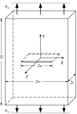
Figure 5.1 A through-thickness center-cracked plate subjected to a uniform far-field displacement ...38

Figure 5.2 One-eighth of the plate to be generated as a finite element model...38

Figure 5.3 Finite element mesh of a one-eighth center-cracked plate (a/w=0.1)...39

Figure 5.4 Mesh refinement near crack front region...39

Figure 5.5 Radius of the outer surface of Ring #12 equals to 100e0...40

Figure 5.6 Sizes of element layers in terms of the half thickness t ...40

Figure 5.7 Configuration and dimensions of a center-cracked panel with stiffeners...41

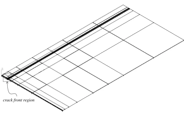
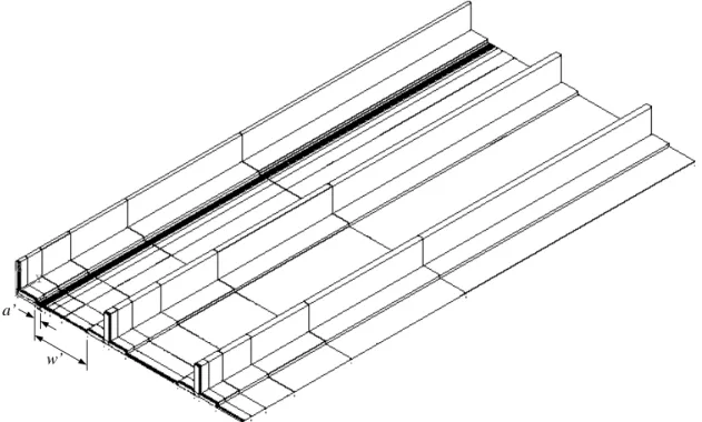
Figure 5.8 The finite element model of a one-fourth center-cracked stiffened panel (a’/w’=0.1) ...41

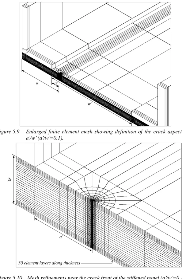
Figure 5.9 Enlarged finite element mesh showing definition of the crack aspect ratio a’/w’ (a’/w’=0.1)...42

Figure 5.10 Mesh refinements near the crack front of the stiffened panel (a’/w’=0.1) ....42

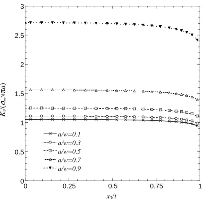
Figure 6.1 Normalized stress intensity factors through half of the thickness for isotropic plates of t=0.165 in. (t/w=0.00825) with various a/w ratios. ...54

Figure 6.2 Normalized stress intensity factors at center of the thickness (x3/t=0) for isotropic plates with two different thicknesses ...54

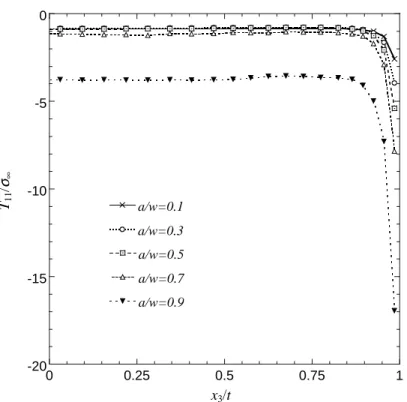
Figure 6.4 Normalized T11 stresses at center of the thickness (x3/t=0) for isotropic plates with two different thicknesses ...55

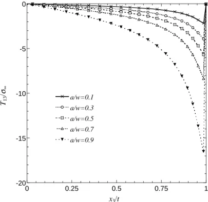
Figure 6.5 Normalized T13 stresses through half of the thickness for isotropic plates of

t=0.165 in. (t/w=0.00825) with various a/w ratios...56

Figure 6.6 Normalized T13 stresses at quarter of the thickness (x3/t=0.5) for isotropic plates with two different thicknesses ...56

Figure 6.7 Normalized stress intensity factors through half of the thickness for isotropic plates of a/w=0.1 with various t/w ratios ...57

Figure 6.8 Normalized stress intensity factors at center of the thickness (x3/t=0) for isotropic plates of a/w=0.1...57

Figure 6.9 Normalized T11 stresses through half of the thickness for isotropic plates of

a/w=0.1 with various t/w ratios...58

Figure 6.10 Normalized T11 stresses at center of the thickness (x3/t=0) for isotropic plates of a/w=0.1 ...58

Figure 6.11 Normalized T13 stresses through half of the thickness for isotropic plates of

a/w=0.1 with various t/w ratios...59

Figure 6.12 Normalized T13 stresses at quarter of the thickness (x3/t=0.5) for isotropic plates of a/w=0.1...59

Figure 6.13 Normalized stress intensity factors through half of the thickness for

orthotropic plates of t=0.165 in. (t/w=0.00825) with various a/w ratios ...60

Figure 6.14 Normalized stress intensity factors at center of the thickness (x3/t=0) for orthotropic plates with two different thicknesses ...60

Figure 6.15 Normalized T11 stresses through half of the thickness for orthotropic plates of t=0.165 in. (t/w=0.00825) with various a/w ratios ...61

Figure 6.16 Normalized T11 stresses at center of the thickness (x3/t=0) for orthotropic plates with two different thicknesses ...61

Figure 6.17 Normalized T13 stresses through half of the thickness for orthotropic plates of t=0.165 in. (t/w=0.00825) with various a/w ratios ...62

Figure 6.18 Normalized T13 stresses at quarter of the thickness (x3/t=0.5) for orthotropic plates with two different thicknesses ...62

Figure 6.19 Normalized stress intensity factors through half of the thickness for

orthotropic plates of a/w=0.1 with various t/w ratios ...63

Figure 6.20 Normalized stress intensity factors at center of the thickness (x3/t=0) for orthotropic plates of a/w=0.1 ...63

Figure 6.22 Normalized T11 stresses at center of the thickness (x3/t=0) for orthotropic plates of a/w=0.1...64

Figure 6.23 Normalized T13 stresses through half of the thickness for orthotropic plates of a/w=0.1 with various t/w ratios ...65

Figure 6.24 Normalized T13 stresses at quarter of the thickness (x3/t=0.5) for orthotropic plates of a/w=0.1...65

Figure 6.25 Normalized stress intensity factors through the thickness for orthotropic stiffened panels of t=0.165 in. (t/w=0.00825) with various a’/w’ ratios ...66

Figure 6.26 Normalized stress intensity factors at center of the thickness (x3/t=0) for orthotropic stiffened panels with various a’/w’ ratios for two thicknesses ...66

Figure 6.27 Normalized T11 stresses through the thickness for orthotropic stiffened panels of t=0.165 in. (t/w=0.00825) with various a’/w’ ratios ...67

Figure 6.28 Normalized T11 stresses at center of the thickness (x3/t=0) for orthotropic stiffened panels with various a’/w’ ratios for two thicknesses ...67

Figure 6.29 Normalized T13 stresses through the thickness for orthotropic stiffened panels of t=0.165 in. (t/w=0.00825) with various a’/w’ ratios ...68

Nomenclature

Latin symbols:

A Complex matrix containing Stroh eigenvectors

A, Aε , A1, A2 Surfaces on a domain

a Half crack length

a’ Half crack length calculated from the edge of the central stiffener to the crack front

B Complex matrix containing Stroh eigenvectors

B Stress biaxiality ratio

C Stiffness matrix

C0 Reduced stiffness matrix

Cij Components of stiffness matrix

E Young’s modulus

EX, EY, EZ Young’s moduli of an orthotropic material

e Expression for manipulation of eigenvalues of elastic constants

e0 Radial size of finite elements attached on crack front

F Total nodal force on one end of a panel (plate)

f Auxiliary line load vector

f Area under the s-function curve

f1 Auxiliary uniform line load normal to crack front

f3 Auxiliary uniform line load parallel to crack front

) (

) (n θ ij

f , f_ij(θ) Functions of the angle of orientation in the asymptotic equation

G Energy release rate

GXY, GYZ, GXZ Shear moduli of an orthotropic material

I Identity matrix

I, I1, I(1), I(2) Values of the interaction integral

i −1

J, J1 Values of J-integral or the equivalent domain integral

K, KI, KII, KIII Stress intensity factors I

K Normalized stress intensity factor

k Vector for local stress intensity factors

kI, kII, kIII Local stress intensity factors

k1, k2, k3 Normalization factors in Stroh formalism

L, L(θ) Barnette-Lothe tensors

l Half panel (plate) length

lc Characteristic length of a finite element mesh

m Expression for manipulation of reduced compliance

Nj Shape function of the j-th node in an element

n unit normal vector

nj The j-th directional component of the unit normal vector

p1, p2 Expressions in Stroh eigenvectors

Q Simplified symbol for terms in J-integral calculation

q1, q2 Expressions in Stroh eigenvectors

r Distance from a crack tip; the first coordinate in a polar coordinate system

S, S(θ) Barnette-Lothe tensors

s Compliance matrix

s0 Reduced compliance matrix

s’ Vector of the derivatives of the s-function

s Spatial weighting function (also called s-function) )

( j

s Value of the s-function on the j-th node of an element

sij Components of compliance matrix ij

s′ Components of reduced compliance matrix

T, Tij Elastic T-stress

T11, T13, T33 Components of T-stress 11

T , T₁₃ Normalized T-stresses

t Half panel (plate) thickness

t Normalized panel (plate) thickness

u Displacement vector

ua Auxiliary displacement vector

ui, uk Components of displacement vector a

i

u Components of the auxiliary displacement field

∞

u Far-field displacement applied on the ends of a panel (plate)

V, Vε Volumes of a domain

W Stress-work density

w Half panel (plate) width

w’ Distance between edges of two adjacent stiffeners

wm, wn, wp Integration weights

X, Y, Z Global Cartesian coordinates in a panel (plate)

x1, x2, x3 Cartesian coordinates of a local (crack front) coordinate system

y1, y2 Real parts of complex numbers

z1, z2 Imaginary parts of complex numbers Greek symbols:

Γ An arbitrary path around a crack tip

∆ Length of a segment of crack front

εc

Contracted strain vector

ε Radius of a small cylindrical volume encompassing a segment of crack front

εi Components of contracted strain vector

εij Components of strain tensor a

ij

ε Components of the auxiliary strain field

ζ The third coordinate in an element coordinate system

η The second coordinate in an element coordinate system

θ Angle of orientation; the second coordinate in a polar coordinate system

ν Poisson’s ratio

νXY, νYZ, νXZ Poisson’s ratios of an orthotropic material

ξ The first coordinate in an element coordinate system

σ Stress tensor

σa

Auxiliary stress tensor

σc

Contracted stress vector

σij Components of stress tensor a

ij

σ Components of the auxiliary stress field

∞

σ Average stress applied on the ends of a panel (plate)

ςα Simplified symbol for expressions associated eigenvalues of elastic constants

φa

Auxiliary stress function

φ1, φ2 Components of auxiliary stress function

1

Introduction

The study of fracture mechanics emerged in the early twentieth century. Among a handful of researchers, Griffith's idea of “minimum potential energy” [1] provided a foundation for all later successful theoretical studies of fracture, especially for brittle materials. But it was not until after World War II that fracture mechanics developed as a discipline. Derived from Griffith's theorem, the concept of energy release rate, G, was first introduced by Irwin [2], and was in a form that is more useful for engineering applications. He defined the energy release rate, or the crack extension force tendency so that it can be determined from the stress and displacement fields in the vicinity of the crack tip rather than from considering an energy balance for the elastic solid as a whole, as Griffith suggested. Irwin also used the Westergaard stress function [3] to show that the stresses and displacements near the crack tip of an isotropic linear elastic material in mode-I plane stress could be described by a single parameter, K, that is related to the energy release rate [4], i.e.,

E K

G = 2 , (1.1)

where E is the Young's modulus. For plane strain, E is replaced by E (1−ν2). This crack tip characterizing parameter later became known as the stress intensity factor.

Rice [5] later defined a path-independent J-integral for two-dimensional crack problems in linear and nonlinear elastic materials. As shown in Figure 1.1, J is the line integral surrounding a two-dimensional crack tip and is defined as

∫

∂ −

= i

j

ij ds

x u n Wdx

J ( )

1

2 σ , i, j = 1, 2 (1.2)

Therefore, the stress intensity factor K can be readily obtained, according to Eq.(1.1) and the computational efficiency of the J-integral, as

JE

K = . (1.3)

The J-integral is effective for evaluating K in two-dimensional crack problems. For three-dimensional problems, however, it is difficult to distinguish K at different x3 locations, assuming the line integral is performed on the x1-x2 plane. Thus an alternative procedure needs to be developed to determine the distribution of K through the thickness. Parks [6] employed the virtual crack extension method to determine J from elastic-plastic finite element solutions. The method is based on an energy comparison of two slightly different crack lengths and requires only one elastic-plastic finite element solution, because the altered crack configuration is obtained by changing nodal positions. The procedure is directly applicable to two-dimensional configurations but can be extended in a straightforward manner to obtain arc-length-weighted average values of J along three-dimensional crack fronts. The three-three-dimensional applications, however, have significant loss of accuracy in the near-tip region where the values of field quantities (stresses, strains, and displacements) are required to determine the point-wise energy release rate along the crack front. Based on the virtual crack extension method, deLorenzi [7,8] developed a finite element method that is more general to calculate the energy release rate in two-dimensional and three-dimensional fracture problems and could include the effects of body forces and traction loading on the crack faces.

theorem and the implementation of a spatial weighting function that is based upon the virtual crack extension method.

With the EDI method, a point-wise value of J along a three-dimensional crack front can be calculated, and therefore the value of K along the crack front can be obtained from Eq.(1.3). Another advantage is that the EDI method transforms surface integrals in a three-dimensional problem into integrals over a volume, or a domain (hence the name of equivalent domain integral), without evaluation of the stress singularities directly on the crack front.

The stress intensity factor alone is not enough to characterize the crack behavior in some cases. Other fracture parameters may be needed to describe the crack behavior more precisely. As Irwin [4] pointed out there is a mathematical expression for crack-tip stress distributions in linear isotropic solids, Williams [22] showed that the expression is in fact an infinite power series of r, where r is the distance from the crack tip. The power series, in a concise form, can be written as

∑

=

1

) ( ) 2 / 1 (

) ( )

, (

n

n ij n n

ij r θ A r f θ

σ , i, j = 1, 2 (1.4)

where An are unknown constants which depend on the geometry and loading conditions, and (n)(θ)

ij

f are the known angular distributions. The mode-I stress intensity factor is included in the first term of Eq.(1.4) as

) ( 2

lim I ( 1)

0 π θ

σ −

→

= ij

r

ij f

r K

, (1.5)

in which the stresses are singular at r=0 and A₁ =K_I 2π . The leading term of the series of Eq.(1.4) represents r-1/2 singularity; the second term is a constant; the third and higher-order terms are proportional to r(1/2)n, n=1,2,3…. Larsson and Carlsson [23] first denoted this constant term as T, and later it became the so-called “elastic T-stress”.

and Carlsson [23] showed that the T-stress is necessary to modify the solution of the stress state in a small-scale yielding crack problem in plane strain condition. Rice [24] showed that T is in fact a constant stress parallel to the crack flank, and included it as a second crack tip parameter to characterize suitably small plane strain yield zones. Several methods have been used to practically determine the T-stress [25]. In addition to the methods mentioned in [25], recently other methods were also used, such as the boundary layer method and the displacement field method [26], as well as the stress difference method [27]. Among those methods, the interaction integral method developed by Nakamura and Parks [28] demonstrated highly computational effectiveness since it is based on the EDI method and has the capability to compute the T-stress not only in an isotropic material but also in an anisotropic material.

Under the NASA Advanced Composite Technology Program, Langley Research Center (LaRC) has performed fracture toughness tests for various types of wing structure specimens made from stitched warp-knit fabric composites. Variations of in-plane geometry and crack length were evaluated from three kinds of specimen geometry [29]: compact tension (CT) specimen with the crack aspect ratios 0.46≤a w≤0.69; center-cracked tension (CCT) specimen with 0.26≤2a w≤0.42; single-edge notched tension (SENT) with 0.25≤a w≤0.34.

Methods based on the equivalent domain integral and Betti’s reciprocal theorem were developed by Yuan and Yang [29] to extract the fracture parameters – critical stress intensity factor and T-stress. With the limited experimental data, the results tend to show that the critical mode-I stress intensity factor provides a satisfactory characterization for engineering applications of fracture initiation in the composite of a given laminate thickness, provided the failure is fiber-dominated and the crack growth follows in a self-similar manner. In addition, the high constraint due to high tensile T-stress may be expected to inhibit the crack extension in the same plane and promote the crack turning.

using the stitched warp-knit composite material. The crack initially extended in a self-similar manner and then turned parallel to the stiffener direction when the crack approached stiffeners (see Figure 1.2). In this dissertation, the effects of the geometrical attributes on the fracture behavior of this panel are investigated by using three-dimensional finite element analysis and linear elastic fracture mechanics to analyze the composites. Due to the high computational efficiency, the equivalent domain integral method is used to calculate the through-thickness KI stress intensity factor and the interaction integral method is adopted to compute the through-thickness T-stress components. The algorithms of the equivalent domain integral and interaction integral are implemented into a single computer program, which reads a set of finite element solutions from a given mesh as the input to determine the distributions of the fracture parameters along the crack front. The composites are modeled as linear, anisotropic, and homogeneous materials. For the purpose of verification and comparison, a similarly cracked plate structure without stiffeners is also analyzed with the same composite material properties as well as an isotropic material.

Figure 1.1 An arbitrary path on which a line integral is to be calculated.

θ

r

x₁ x₂

Figure 1.2

The cracked stiffen

2

Equivalent Domain Integral (EDI)

The derivation will assume a traction-free crack in a linear elastic material, with the intention of determining the mode-I stress intensity factor KI through the thickness.

2.1

Mathematical Formulation

Let us consider a small cylindrical volume with radius ε encompassing a segment of crack front of length ∆ such that both ε and ∆ approach zero, as shown in Figure 2.1. A local coordinate system is defined so that the axes x1 and x2 are perpendicular to the crack front, while x1 and x3 are lying on the crack plane. The volume is enclosed by five areas, namely the outer surface Aε, two end surfaces Aε1 and Aε2, the top crack surface Aεct, and the bottom crack surface Aεcb.

The local J-integral over the outer surface Aε of the tube is defined as [30]

dA n x u Wn

J i _j

ij

∫

∂ − ∆

=

→ →

∆ ( )

1 lim

1 1

0

0 σ

ε

. i, j = 1, 2, 3 (2.1)

In Eq.(2.1), W is the stress-work density, defined as W =

∫

For the purpose of simplicity in later derivations, let

j i ij n

x u Wn

Q

1 1

∂ ∂ −

= σ . (2.2)

surface integral as

    

  

+ +

∆

=

∫

∫

∫

+ +

→→ ∆

cb ct A

A A

A A

QdA QdA

QdA J

ε ε ε

ε ε

ε 1 2

1 lim

0

0 . (2.3)

The evaluation of surface integrals in Eq.(2.3) is tedious and could lead to errors because singular terms on the crack front are included for numerical integration. Therefore, a modified form of the surface integrals is desirable, and this modified form would be the equivalent domain integral.

Now consider two tubular surfaces, A and Aε , as shown in Figure 2.2. A is an arbitrary surface enclosing Aε on which the J-integral is calculated. A1 and A2 are end surfaces connecting A and Aε . (A-Aε)ct and (Aε-A)cb denote the top and bottom crack surfaces between A and Aε, respectively. An enclosed volume (V-Vε) is surrounded by all of these surfaces, which are called collectively A_Σ, defined as

2 1 ) (

)

(A A A A A A

A A

AΣ = − ε + − ε ct + ε − cb+ + . (2.4)

Based on the virtual crack extension theory, deLorenzi [8] proposed the concept of virtual node shift that forms the definition of a spatial weighting function, which is called s-function by some researchers [12-16,30]. We will adopt this name throughout this dissertation and use the symbol s to represent this spatial weighting function.

According to the configuration shown in Figure 2.2, an arbitrary but continuous s-function is defined between A and Aε so that the function has the following properties:

0 ) , ,

(x₁ x₂ x₃ =

s on A, Aε1 and Aε2, A1 and A2; (2.5a)

) ( ) , ,

(x1 x2 x3 s x3

s = on Aε. (2.5b)

        + + + − =

∫

∫

∫

∫

Σ A A ct A Acb A A Act Acb

A QsdA QdA QsdA QsdA f J ε ε ε ε ε

ε) ( ) 1 2

(

1

. (2.6)

In Eq.(2.6) f is the area under the s-function curve on surface Aε and is defined as

∫

∆

= s(x3)dx3

f . (2.7)

The s-function is equal to zero on both end surfaces of Aε1 and Aε2; therefore, 0 2 1 =

∫

QsdA and Eq.(2.6) remains as

        + + − =

∫

∫

∫

Σ A A ct A Acb Act Acb

A QsdA QsdA QsdA f J ε ε ε ε) ( ) ( 1 . (2.8)

In Eq.(2.8) the negative sign of the first integral, which is over an enclosed domain, comes from the opposite direction of the outer normal vector to the surface Aε of the volume (V-Vε) in comparison with the normal vector to the surface Aε in Figure 2.1. The other integrals in Eq.(2.8) are actually on the crack surfaces. Therefore, we may separate integrals in Eq.(2.8) into a “domain” integral and a “crack face” integral, denoted as

[

]

1

J J

f

J = + , (2.9)

where

∫

Σ − =

A

QsdA J)_domain

( , (2.10)

and =

∫

∫

∫

+ − + − sdA Q QsdA QsdA J cb ct cb

ct A A A A

A A face crack ) ( ) ( face crack ) ( ε ε ε ε . (2.11)

By recalling Eq.(2.2), Eq.(2.10) can be written as

∫

ij s n dA

x u Wsn J 1 1 domain )

( σ . (2.12)

sdV x x W dV x s x u x s W J V V ij ij V V j i ij

∫

∫

( . (2.13)

Since the analysis is limited to linear elastic materials, it can be shown that the second integral in Eq.(2.13) is equal to zero [13]. Thus Eq.(2.13) is simplified as

dV x s x u x s W J V V j i ij

∫

( . (2.14)

On the crack surfaces, the first and third directional components of the unit normal vector n are equal to zero (n1 =n3 =0), according to the local coordinate system. The second component of n has the properties of n₂ =+1 on the bottom face and

1

2 =−

n on the top face. Upon substituting these conditions into Eq.(2.2), we have

    ∂ ∂ + ∂ ∂ + ∂ ∂ − = 2 1 3 32 2 1 2 22 2 1 1 12 1 face

crack n

x u n x u n x u Wn

Q σ σ σ . (2.15)

Since 0σ₂₂ =σ₃₂ = on the crack surfaces, Eq.(2.15) is then reduced to

2 1 1 12 face

crack n

x u Q ∂ ∂ −

= σ . (2.16)

For a traction-free crack surface, σ12 =0. Thus the value of Q in Eq.(2.16) is equal to

zero, and all integrals in Eq.(2.11) vanish.

Therefore, for a traction-free crack in a linear elastic material, the equivalent domain integral for the determination of KI, in terms of displacements, strains, and stresses, can be conveniently expressed as

dV x s x u x s W f J V j i ij

∫

σ . (2.17)

2.2

Numerical Implementation

The 20-node isoparametric brick-shaped elements are frequently used in the three-dimensional finite element analysis of linear elastic crack problems. The typical finite element mesh around the crack front is a fan-type mesh, as shown in Figure 2.3. The shaded area indicates a domain over which the equivalent domain integral is calculated. All elements in and beyond this domain are 20-node elements. The wedge-shaped elements attached on the crack front, however, contain only 15 nodes for each element.

The J-integral is the sum of the domain integral contributed by each element in the designated domain, e.g., the shaded area in Figure 2.3. That is,

∑

( , (2.18)

where (J )i is the volume integral over the i-th element, and ne is the number of elements

enclosed in the domain.

In finite element modeling, the displacements are expressed by shape functions and nodal displacements:

∑

k N u

u , k = 1, 2, 3 (2.19)

where N_j = N_j(ξ,η,ζ) is the element shape function for a three-dimensional solid element, and ξ, η, ζ are the element’s local coordinates that range between ±1. (u )_{k j} is the displacement component at the j-th node where j is the local node number within an element. Then for the volume integral of a single element, Eq.(2.17) can be written as

[ ]

σ d d d

x s x u x s W f J k j jk

i detJ

1 ) ( 1 1 1 1 1 1 1 1

1

∫ ∫ ∫

− − −     ∂ ∂ ∂ ∂ − ∂ ∂ −

= . (2.20)

[ ]

i m n p

p n m x

i w w w

x s W f J             _{− ′ ′} ∂ ∂ − =

∑∑∑

1 ₁ . (2.21)

In Eq.(2.21), W is the stress-work density, T

1

x

u′ is the vector of displacement derivatives,

σ is the stress tensor, s’ is the derivatives of the s-function, and det[J] denotes the determinant of the Jacobian matrix. wm, wn, and wp are integration weights, and they all have the values of unity for 2×2×2 reduced integration [31].

Eq.(2.21) is the equation to be used for computation; therefore, the numerical implementation of each item in this equation needs to be explicitly expressed, as shown in the following sections. Once all items in Eq.(2.21) can be readily calculated, the J-integral over the domain can be evaluated from Eq.(2.18).

2.2.1

The Jacobian Matrix

The Jacobian matrix is defined by

                ∂ ∂ ∂ ∂ ∂ ∂ ∂ ∂ ∂ ∂ ∂ ∂ ∂ ∂ ∂ ∂ ∂ ∂ = ζ ζ ζ η η η ξ ξ ξ 3 2 1 3 2 1 3 2 1 x x x x x x x x x

J . (2.22)

Each component of the matrix, according to the finite element theory, is defined as

∑

ξ , k = 1, 2, 3 (2.23a)

∑

k N _x

x

η

η , k = 1, 2, 3 (2.23b)

∑

ζ , k = 1, 2, 3 (2.23c)

2.2.2

The Stress Tensor and Stress-Work Density

The stress tensor σ of a linear elastic material is a 3×3 symmetric matrix shown as

        = 33 23 13 23 22 12 13 12 11 σ σ σ σ σ

σσ σ σ . (2.24)

The stress-work density of the linear elastic material is (σ_ijε_ij) 2, or

(

)

2 1 ε σ ε σ ε σ ε σ ε σ ε σ + + + + + =

W . (2.25)

Note that σij and εij are the stress and strain components from the finite element solutions output on the integration points.

2.2.3

The Derivatives of the s-Function

s’ is the vector containing derivatives of the s-function with respect to the local

coordinate system and is expressed as T 3 2 1       ∂ ∂ ∂ ∂ ∂ ∂ = ′ x s x s x s

s . (2.26)

To evaluate Eq.(2.26), the s-function must be defined first. Since the s-function is arbitrary and satisfies Eq.(2.5), it can be conveniently defined by the sums of the element shape functions as

∑

s ξ η ζ . (2.27)

It is clear that the s-function is a function of the element coordinate system (ξ, η,

ζ), rather than the crack front coordinate system (x1, x2, x3). Thus s’ should be expressed in terms of (ξ, η, ζ) before it can be evaluated. This can be done by the chain rule, as shown in the following equation:

                  ∂ ∂ ∂ ∂ ∂ ∂ =                   ∂ ∂ ∂ ∂ + ∂ ∂ ∂ ∂ + ∂ ∂ ∂ ∂ ∂ ∂ ∂ ∂ + ∂ ∂ ∂ ∂ + ∂ ∂ ∂ ∂ ∂ ∂ ∂ ∂ + ∂ ∂ ∂ ∂ + ∂ ∂ ∂ ∂ =                   ∂ ∂ ∂ ∂ ∂ ∂ = ′ − ζ η ξ ζ ζ η η ξ ξ ζ ζ η η ξ ξ ζ ζ η η ξ ξ s s s x s x s x s x s x s x s x s x s x s x s x s x s 1 3 3 3 2 2 2 1 1 1 3 2 1 J

s . (2.28)

J-1 is the inverse Jacobian matrix containing the following components:

3 3 3 2 2 2 1 1 1 1                   ∂ ∂ ∂ ∂ ∂ ∂ ∂ ∂ ∂ ∂ ∂ ∂ ∂ ∂ ∂ ∂ ∂ ∂ = − x x x x x x x x x ζ η ξ ζ η ξ ζ η ξ

J . (2.29)

The derivatives of the s-function with respect to the element coordinate system, i.e.

ξ ∂ ∂s , η ∂ ∂s and ζ ∂ ∂s

in Eq.(2.28), can be evaluated in the same manner as Eq.(2.23).

2.2.4

The Derivatives of the Displacements

T

1

x

u′ is the vector of displacement derivatives and can be expressed as

      ∂ ∂ ∂ ∂ ∂ ∂ = ′ 1 3 1 2 1 1 T 1 x u x u x u x

u . (2.30)

( )j

j j

j

k _u

x N

x N

x N

x u

∑

 

∂ ∂ ∂ ∂ + ∂ ∂ ∂ ∂ + ∂

∂ ∂ ∂ = ∂

∂ 20

1 1 1 1

1

ζ ζ η η ξ

ξ . k = 1, 2, 3 (2.31)

In Eq.(2.31), 1

x

∂ ∂ξ

, 1

x

∂ ∂η

and 1

x

∂ ∂ζ

are the components of the first row of the inverse

Jacobian matrix of Eq.(2.29);

ξ

∂ ∂Nj

,

η

∂ ∂Nj

and

ζ

∂ ∂Nj

Figure 2.1 A small cylindrical volume around a segment of crack front, with the local coordinate system shown.

Figure 2.2 A domain enclosing a segment of crack front.

x1

x2

x3

ε ∆

Aε

Aεct

Aε2

Aεcb

Aε1

crack front

ε ∆

s-function x1

x2

x3

Aε

A1

A

A2

V-Vε

(Aε-A)cb

Figure 2.3 The schematic finite element mesh near a segment of the crack front.

Figure 2.4 A 20-node element with the associated s-functions.

x1

x3

x2

x1

x2

x3

∆ 2

3 5

6

7

8

4 10

11 13

14 ₁₅

16

20

19 18

1

9 ₁₂

17

3

Interaction Integral

The interaction integral is necessary for extracting the elastic T-stress from an existing finite element solution. It is based upon the formulation of the EDI method as well as a superimposed auxiliary stress field. Kfouri [32] gave the auxiliary stress field that is the analytical solution corresponding to a point force applied to a crack tip and parallel to the crack surface under plane strain in isotropic solids. For a three-dimensional crack, the point force becomes a uniform line load that is applied along the crack front, as shown in Figure 3.1(a). This stress field is a function of r, the distance from the crack front, and θ, the angle from x1 axis toward x2 axis; but it is independent of the crack front location x3.

Nakamura and Parks [28] applied the auxiliary stress field with the interaction integral and successfully calculated the T-stress distribution along the three-dimensional crack front. The auxiliary stress field, however, is valid only for isotropic materials. For anisotropic materials, the corresponding auxiliary fields have been derived using Stroh formalism [34].

Similar to Eq.(2.17) of the equivalent domain integral, the interaction integral for mode-I loading ina given domain may be expressed as

dV x s x u x u x s f I V j i ij i ij ij ij

∫

1 _{σ ε σ σ}

, i, j = 1, 2, 3 (3.1)

where σija, a ij

ε , and u are the components of the auxiliary stress, strain, andia

displacement fields, respectively. For the purpose of numerical integration of each individual element in a domain, Eq.(3.1) can be written similarly to Eq.(2.21) as

(

)

[ ]

i m n p

p n m x x jk jk

i w w w

x s f I               _{+ ′ + ′ ′} ∂ ∂ − =

∑∑∑

u ) det

( 1 ) ( 2 1 2 1 2 1 a T T a 1 a

1 σ ε 1 1 . (3.2)

fields, respectively. εa_jk are components of the auxiliary strain tensor. These entities are expressed in terms of the components of the associated tensor or vector as follows:

          = a 33 a 23 a 13 a 23 a 22 a 12 a 13 a 12 a 11 a σ σ σ σ σ σ σ σ σ ; (3.3)

(

)

13 13 a 23 23 a 12 12 a 33 33 a 22 22 a 11 11 a

2σ ε σ ε σ ε

ε σ ε σ ε σ ε

σjk jk = + + + + + ; (3.4)

      ∂ ∂ ∂ ∂ ∂ ∂ = ′ 1 a 3 1 a 2 1 a 1 T a 1 ) ( x u x u x u x

u . (3.5)

Quantities of Eq.(3.3) and Eq.(3.4) can be obtained by straightforward substitution of auxiliary stress and strain fields. Components in Eq.(3.5) can be computed similarly to Eq.(2.31) as

( )

1 1 1 1

1 a

∑

ξ , k = 1, 2, 3 (3.6)

where u are components of the auxiliary displacement vector. All of the other items notka

associated with the auxiliary fields are calculated exactly in the same way as the equivalent domain integral is.

Let us recall the Williams expansion of Eq.(1.4) which can be generalized to three-dimensional problems. It is assumed that the asymptotic expansion of the stress field near the crack front location under general loading conditions can be expressed as

) 1 ( )

( 2

III) ( 3

I) ( 1

) (

o T f

r k

ij n

n ij n

ij =

∑

=

θ π

σ , i, j = 1, 2, 3 (3.7)

where kI, kII, and kIII are local stress intensity factors, ( ) ) (n θ ij

f are angular distributions for the crack-tip field given by the two-dimensional deformation of anisotropic elasticity theory, and o(1) represents other higher order terms. Tij are the non-singular T-stresses, which have three distinct components, namely

[ ]

  

   =

33 13

13 11

0 0 0 0

0

T T

T T

Tij . (3.8)

T11 is obviously the stress component acting parallel to the crack plane [24] and can be determined by the interaction integral with an imposed uniform line load f1 as shown in Figure 3.1(a). Similarly T13 can be determined by using a different set of auxiliary fields. Instead of the line load perpendicular to the crack front and the x2-x3 plane, a constant force f3 in x3-direction and through the full length of crack front should be imposed. This configuration, as shown in Figure 3.1(b), will yield an auxiliary stress field necessary to extract T13. T33 is a combination of T11 and T13 and can be readily obtained after the other two T-stresses are determined (see Chapter 4).

In the following sections, the derivations of both types of auxiliary fields are presented in order to determine all of the T-stress components.

3.1

Auxiliary Fields for T

direction out of plane [34]. Since most composite plates have at least one symmetry plane at x3=0, we will limit the derivation under this restriction. This kind of material is called the monoclinic material with the plane of symmetry at x3=0, or simply the monoclinic material about x3=0.

The generalized Hooke’s law states the stress-strain relation in contracted notation as

c c

C

= , (3.9)

where c =

[

] [

]

(3.10)

and

[

] [

]

T 6 5 4 3 2 1 c 2 2

2ε ε ε

ε ε ε ε ε ε ε ε ε =

= . (3.11)

C is a 6×6 matrix, and is called the stiffness matrix in which the components Cij are material properties. A monoclinic material about x3=0 has the following form of the stiffness matrix:                 = 66 36 26 16 55 45 45 44 36 33 23 13 26 23 22 12 16 13 12 11 0 0 0 0 0 0 0 0 0 0 0 0 0 0 0 0 C C C C C C C C C C C C C C C C C C C C

C . (3.12)

The inverse of the stress-strain relation defines the compliance matrix s, as c

c

s

= , (3.13)

where s is the inverse of C. Thus the compliance matrix of a monoclinic material about

x3=0 has the form of

                = = − 66 36 26 16 55 45 45 44 36 33 23 13 26 23 22 12 16 13 12 11 1 0 0 0 0 0 0 0 0 0 0 0 0 0 0 0 0 s s s s s s s s s s s s s s s s s s s s C

s . (3.14)

equation for σ3 in Eq.(3.9), the stress-strain relation of the monoclinic material can be written as

[

]

[

]

5 4 6 2 1 0 T 5 4 6 2

1 σ σ σ σ ε ε ε ε ε

σ =C , (3.15)

where C0 is the reduced stiffness matrix, shown as

              = 55 45 45 44 66 26 16 26 22 12 16 12 11 0 0 0 0 0 0 0 0 0 0 0 0 0 C C C C C C C C C C C C C

C . (3.16)

The inverse of Eq.(3.16) gives the definition of the reduced compliance matrix s0, as

( )

s . (3.17)

The components of s0 can be also obtained by solving for σ3 in the third equation of Eq.(3.13) that will yield

∑

s . β ≠3 (3.18)

Substituting Eq.(3.18) into the other five equations of Eq.(3.13) will have

33 3 3 s s s s

sij′ = ij − i j . i, j = 1, 2, 4, 5, 6 (3.19)

According to Stroh formalism for two-dimensional deformations of an anisotropic elastic body [35], the characteristic equations have the reduced compliance as coefficients: 0 2 ) 2 (

2 ₁₆ 3 _{12 66} 2 _{26 22}

4

11′ − s′ + s′ +s′ − s′ +s′ =

s µ µ µ µ ; (3.20a)

0

2 _{45 44}

2

55′ − s′ +s′ =

s µ µ . (3.20b)

The solutions to Eq.(3.20) are the eigenvalues of elastic constants, µα (α = 1, 2, 3), where

complex numbers, and µ_α are the conjugates of µα.

Under the uniform line load f1 shown in Figure 3.1(a), the auxiliary stresses are inversely proportion to r, or a ∝ −1

r

ij

σ . In Stroh formalism, the real form solution for the displacement ua and the stress function φa due to the point forces can be written as

f L S I

ua ln ( ) 1

2 −     ₊ − = θ π r , (3.21a) f L L 1 a ) ( =

2φ θ − , (3.21b)

where S and L are Barnette-Lothe tensors, S(θ) and L(θ) are their associate tensors, f is the vector of the line load per unit thickness, and I is the 3×3 identity matrix. These items are defined as follows:

T 1 0 0] [ f

=

f ; (3.22)

(

)

{

}

sin cos ln Re 2 )

( A B

S θ µ θ

π

θ = + α ; (3.23a)

(

)

{

}

sin cos ln Re 2 )

( B B

L θ µ θ

π

θ =− + α ; (3.23b)

( )

L . (3.24)

The definitions of the terms in Eq.(3.23) and Eq.(3.24) are given as follows.

For the purpose of simplicity, let ς_α=cosθ+µ_αsinθ. In Eq.(3.23), implies a diagonal matrix, thus

(

)

θ α . (3.25)

        ′ − ′ = ) ( 0 0 0 0 3 44 45 3 2 2 1 1 2 2 1 1 µ s s k q k q k p k p k

A and (3.26a)

        − − − = 3 2 1 2 2 1 1 0 0 0 0 k k k k

k µ µ

B , (3.26b)

where p1, p2, q1, q2 can be obtained from 12

16 2

11 s s

s

p_α = ′ µ_α − ′ µ_α + ′ and q_α =s₁₂′ µ_α −s₂₆′ +s₂₂′ µ_α . α = 1, 2 (3.27)

k1, k2, k3 are normalization factors satisfying the following relations: 1

) (

2 1 1 1

2

1 q − p =

k µ ; 12 ( 2 2 2)

2

2 q − p =

k µ ; 2 ( 44 3 45) 1

2

3 s′ −s′ =

k µ . (3.28)

The components of L-1 in Eq.(3.24) are defined by the following relations: i

z y_{1 1} 2

1+µ = +

µ ; (3.29a)

i z y_{2 2} 2

1µ = +

µ ; (3.29b)

1 2 2 1z y z y

e= − ; (3.29c)

(

)

45 45 55 44 − ′ ′ − ′ ′

= s s s s

m . (3.29d)

Upon substitution of Eq.(3.22) through Eq.(3.24), the stress function of Eq.(3.21b) can be obtained as

        ′ − = 0 Re ₂ 1 11 1

a φφ

π

s f

φ , (3.30)

where

(

) (

)

2 2 1 1 2 1 2 2 2 2 2 2 1 2 1 2 1 1

1 µ lnς µ lnς µ lnς µ lnς

φ = z k +k −z k +k (3.31a)

and φ₂ =−z₁

(

) (

)

To determine the auxiliary stress field from the stress function, let tr be the traction vector on a cylindrical surface of r = constant which can be obtained as [33]

θ φ ∂ ∂ − = r r 1

or         ′ = 0 Re 2 1 11 1 r r r t t r s f π

t , (3.33)

where

(

) (

)

2 2 1 1 2 1 2 2 2 2 2 2 1 2 1 2 1 1

1 = z k µ Ω +k µ Ω −z k µ Ω +k µ Ω

tr (3.34a)

and ₁

(

) (

)

2 =−z k Ω +k Ω +z k Ω +k Ω

t_r µ µ . (3.34b)

In Eq.(3.34) Ω_α is defined as

θ µ θ θ µ θ ς θ θ α α α α sin cos cos sin ln ) ( + + − = ∂ ∂ =

Ω . α = 1, 2, 3 (3.35)

Then the stresses in the cylindrical coordinate system are

[

]

rr cosθ sinθ 0t

σ = ; (3.36a)

[

]

r3 = 0 0 1t

σ ; (3.36b)

0 3 =

=

= θ θ

θθ σ σ

σ r . (3.36c)

σr3 is found to be equal to zero after substituting Eq.(3.33) into Eq.(3.36b). Substitution of Eq.(3.33) into Eq.(3.36a) also gives σrr, which is a function of r and θ, as

{

}

π

σ Re cos sin

2 1 11 1 r r

rr t t

r s

f ′ ₊

= . (3.37)

It should be noted that the auxiliary fields in the calculation of the interaction integral of Eq.(3.1) are all in the Cartesian coordinate system. Hence the auxiliary stresses σ_ija must be obtained by applying coordinate transformation on Eq.(3.36). The results, which will be able to be implemented into the numerical computing procedure, are given as follows:

{

}

π θ

σ cos Re cos sin

2 1 2 11 1 a

11 tr tr

r s f

+ ′

= ; (3.38a)

{

}

π θ

σ sin Re cos sin

2 1 2 11 1 a

22 tr tr

r s f

+ ′

= ; (3.38b)

{

}

π

θ θ

σ sin cos Re cos sin

2 1

11 1 a

12 tr tr

r s f

+ ′

= ; (3.38c)

0 a 23 a

13 =σ =

a 33

σ can be obtained by substitution of Eq.(3.38) into Eq.(3.18), which yields

(

_{) {}

_}

π

θ θ

σ cos sin Re cos sin

2 1 33 2 23 2 13 11 1 a

33 tr tr

rs s s

s

f ′ + ₊

−

= . (3.38e)

Once the auxiliary stress field is available, the auxiliary strain field can be readily obtained from the inverse of the stress-strain relation of Eq.(3.13).

The auxiliary displacement field is readily available from Eq.(3.21a) which, after a series of substitution of Eq.(3.22) through Eq.(3.24), will yield u₃a =0 and non-zero items of u and ₁a u as₂a

            + + +       ′ − =       22 2 21 1 12 2 11 1 2 1 11 1 a 2 a

1 _{ln 2Re}

2 zS z S

S z S z r z z s f u u

π , (3.39)

where S11, S21, S12, and S22 are components of S(θ) and are defined as 2 2 2 2 2 1 1 1 2 1

11 k µ p lnς k µ p lnς

S =− − ; (3.40a)

2 2 2 2 1 1 2 1

12 k p lnς k p lnς

S = + ; (3.40b)

2 2 2 2 2 1 1 1 2 1

21 k µ q lnς k µ q lnς

S =− − ; (3.40c)

2 2 2 2 1 1 2 1

22 k q lnς k q lnς

S = + . (3.40d)

Without loss of generality, the magnitude of the line load may be chosen as f1=1 as f is arbitrary. This assumption, as well as the information on material properties and nodal coordinates, will enable the calculation of the auxiliary fields necessary for the evaluation of the interaction integral, which in turn will determine T11.

The auxiliary stress field for T11 in an isotropic material was given by Nakamura and Parks [28] as

θ π

σa 1 3

11 cos

r f

−

= ; (3.41a)

θ θ π

σa 1 2

22 cos sin

r f

−

θ θ π

σa 1 cos2 sin 12

r f

−

= ; (3.41c)

θ ν π

σa 1 cos

33

r f

−

= ; (3.41d)

0 a 23 a

13 =σ =

σ . (3.41e)

It can be shown from strain-displacement relations that the auxiliary displacement field is

(

)

(

)

1 2 ₁ 2

a

1 r

E f

u ; (3.42a)

(

_{) ( )}

_[

_]

πν 1 2 sin cos

2

1 1

a

2 − −

+ − =

E f

u ; (3.42b)

0 a 3 =

u . (3.42c)

3.2

Auxiliary Fields for T

The approach to determine the auxiliary fields for T13 is similar to that of T11, except the line load f1 is replaced by a constant force f3 in the x3-direction, as shown in Figure 3.1(b). This configuration will change the line load vector f in Eq.(3.22) as

T 3] 0 0 [ f =

f , (3.43)

which will yield a different stress function as

        − = 3 2 3 3 a ln 0 0 Re ς

πm k

f

φ . (3.44)

By applying a similar derivation following Eq.(3.32) and Eq.(3.36), the auxiliary stresses in the polar coordinate system can be obtained as

{ }

3 = Rek Ω

mr f

r π

σ , (3.45a)

0 3 = =

=

=σr σ σrr

σθθ θ θ . (3.45b)

Note that Ω3 is obtained through the definition of Eq.(3.35).

a 11

σ , σ₁₂a , and σ₂₂a all are equal to zero because σ_θθ =σ_rr =σ_rθ =0. The transformation of σr3, and σθ3 is conducted by the following relation [36]:

          − =       3 3 23 13 cos sin sin cos θ σσ θ θθ θ σ

σ r _{. (3.46)}

This operation yields the non-zero auxiliary stress components

{ }

σ , (3.47a)

{ }

σ . (3.47b)

Then σ33a can be obtained by the use of Eq.(3.18) that also shows 0 a 33 =

σ . This operation assumes a monoclinic material about x3=0 by using its compliance components shown in Eq.(3.14).

The auxiliary strain field is also readily obtained from the inverse of the stress-strain relation of Eq.(3.13). And the auxiliary displacement field is available from Eq.(3.21a) as well. But with a different f, both u and 1a

a 2

u will be equal to zero while only

a 3

u is the non-zero displacement as

{ }

(

)

3 a

3 ln Reln

2π + ς

−

= r

m f

u . (3.48)

The magnitude of the constant force may also be chosen as f3=1 because f is arbitrary. Hence the auxiliary fields can be calculated, and therefore the T13 for a monoclinic material about x3=0 will be determined.

For an isotropic material, the auxiliary fields may be obtained by applying the material properties on the stiffness matrix of Eq.(3.12). A similar derivation will yield

r f π θ σ 2 cos 3 a

13 =− , (3.49a)

r f π θ σ 2 sin 3 a

0 a 12 a 33 a 22 a

11=σ =σ =σ =

σ ; (3.49c)

(

)

E f

ua 3 1 ln

3 _π

ν + −

Figure 3.1 Auxiliary line load on a three-dimensional crack: (a) uniform forces f1

normal to crack front; (b) uniform forces f3 parallel to crack front.

Figure 3.2 Locations of the integration points inside an element.

x2

x3

x1

x1

x3

x2

uniform forces f1

crack front θ

r

(a) (b)

uniform forces f3

crack front θ

r

1 2 3

4

5 6

7

8 η

ξ ζ

ξ ξ

η η

ζ ζ

5 6

7 8

8 7

3 4 4 1

5 8

1 1

3 1

4

Stress Intensity Factor and T-Stress

The formulations regarding the equivalent domain integral and the interaction integral are implemented into a FORTRAN computer program, which uses the finite element solutions computed from another ANSYS program as the input. Once the equivalent domain integral and the interaction integral are evaluated, the stress intensity factor and T-stresses can be determined. In the following sections, formulation to determine both parameters will be shown in terms of those integral quantities and appropriate material properties. These formulations can be easily implemented into the FORTRAN program as well. The full contents of the ANSYS and FORTRAN programs are provided in the Appendices.

4.1

Stress Intensity Factor

For an anisotropic cracked solid, the energy release rate G is related to the stress intensity factor through [29,33,37]

k L kT 1

2

1 ₋

=

G , (4.1)

where kT =

[

]

G is equal to the value of J-integral. For a pure mode-I crack in an elastic material, kII =

kIII = 0, and Eq.(4.1) will reduce to )

( 2 )

( 3

2 I 11 3

1 k x

e s x

J = ′ , (4.2)

where x3 is the crack front location defined in Section 2.1, and J1(x3) is value of the equivalent domain integral, as defined in Eq.(2.17), on this location. Therefore the local stress intensity factor kI(x3) can be determined as

e s

x J x

k

11 3 1 3

I

) ( 2 ) (

′

For an isotropic material, L-1 has the form of

(

)

L . (4.4)

The Eq.(4.3) will become

2 3 1 3 I 1 ) ( ) ( ν −

= EJ x

x

k , (4.5)

which is the plane strain condition as shown in Eq.(1.3).

4.2

T-Stress

The T-stress, in general, includes three components, namely T11, T13 and T33, as shown in Eq.(3.8). T11 and T13 should be determined from the evaluation of interaction integrals, while T33 can be readily obtained after T11 and T13 are computed.

Let I(1) and I(2) be the values of interaction integral of Eq.(3.1) when the superposed uniform load is f1 and f3, respectively. For an anisotropic material, it can be shown that the following relation between T-Stress and interaction integral exists [37]:

            ₋ =           ′ ′ ′ ′ 3 3 ) 2 ( 3 33 33 13 1 3 ) 1 ( 13 11 55 15 15 11 ) ( ) ( ) ( f x I x s s f x I T T s s s s ε , (4.6)

where ε33(x3) is the crack front extension strain at a given crack front location x3. I(1)(x3) and I(2)(x3) are the interaction integrals on the domain at x3 due to f1 and f3, respectively. Then T11 and T13 at the same crack front location may be expressed as

            ₋     ′ ′ ′ ′ =       − 3 3 ) 2 ( 3 33 33 13 1 3 ) 1 ( 1 55 15 15 11 3 13 3 11 ) ( ) ( ) ( ) ( ) ( f x I x s s f x I s s s s x T x T ε . (4.7)