Designing and Using Views
To Improve Performance of Aggregate Queries
(September 9, 2004)
Foto Afrati1
, Rada Chirkova2
, Shalu Gupta2
, and Charles Loftis2
1
Computer Science Division, National Technical University of Athens, 157 73 Athens, Greece
2
Computer Science Department, North Carolina State University, Raleigh, NC 27695, USA
{chirkova,sgupta5,celoftis}@csc.ncsu.edu
Abstract. Data-intensive systems routinely use derived data, such as indexes or materialized views, to improve query-evaluation performance. In this context, the problem ofdesigning derived datais as follows: Given a set of queries and a database, return definitions of derived data that, when materialized in the database, would reduce the evaluation costs of the queries. Designing materialized views and indexes is an important part of
automated query-performance tuning in data-management systems that experience changes over time, where a system addresses the performance requirements of current frequent and important queries by periodically reconsidering and rematerializing the stored derived data.
In this paper we present an extensible system architecture for Query-Performance Enhancement by Tuning (QPET). QPET combines design and use of derived data in an end-to-end approach to automated query-performance tuning, and selects appropriate data-design algorithms depending on the characteristics of the prevalent queries. Our focus in automated query-performance tuning is on a tradeoff between the amount of system resources spent on designing derived data and the degree of the resulting improvement in query perfor-mance. We present algorithms and experimental results in designing and using materialized views for practically important classes of aggregate queries, including range-aggregate queries on star-schema data warehouses.
Keywords: Data warehouses, query language and query optimization, query processing, materialized views.
1 Introduction
Derived data, such as materialized views or indexes, are routinely used in data-intensive systems to improve query-evaluation performance. In this context, the problem ofdesigning derived data is as follows: Given a set of queries, a database, and a set of constraints on derived data (e.g., a storage limit), return definitions of derived data that, when materialized in the database, would satisfy the constraints and reduce the evaluation costs of the queries. Automated design of materialized views and indexes to answer queries is an important component of automated query-performance tuning in data-management systems that change over time, where a system addresses the performance requirements of current frequent and important queries by periodically reconsidering and rematerializing the stored derived data. For this reason, developing techniques for designing materialized views and indexes to improve query-answering performance is a recognized research direction within the discipline of self-administering database systems [1–3]. In this paper we describe our approach within this research direction and discuss its implementation and validation in our extensible system architecture for Query-Performance Enhancement by Tuning (QPET) [4].
time. One reason is, in many practical scenarios the amount of time or other system resources available for designing derived data is limited. The problem is even more pronounced when, under a requirement to provide continuous services to customers, a system cannot go down for redesign of the stored materialized views or indexes.
We study design and use of materialized views and indexes in automated query-performance tuning in relational data-management systems where the set of prevalent queries changes over time. Our objective is to minimize the evaluation costs of a given query workload subject to given restrictions on design time, by designing and using derived data. To address the tradeoff between the time allotted for designing derived data and the quality of the resulting views or indexes, our approach is to develop specialized algorithms for specific practically important query types. For each type of queries, when designing derived data we use information about how the resulting materialized views or indexes will be used to evaluate the workload queries, that is, at the design stage we use information about rewriting the queries using the outputs of the design stage. In this paper we present techniques for designing and using materialized views; the techniques are applicable to a practically important class of range-aggregate queries on star-schema data warehouses. In the experimental results reported in this paper we use a greedy algorithm BPUS introduced in [7]. We say “workload of star-schema queries” to refer here to a set of aggregate queries where all queries have the same FROM clause and the same join conditions in the WHERE clause.3
To design aggregate views for a workload of star-schema queries, BPUS explores iteratively views in aview lattice, which is a representation of the search space of views for the workload, with directed edges between views denoting which view can be evaluated using another view. At each step, BPUS selects from the lattice a view with the greatest benefit, that is, a view that reduces the most the average cost of answering a query, per unit space. For any materialized view designed by the BPUS algorithm of [7], if the view is usable in evaluating some query, then the answer to the view is the only relation needed in the evaluation. That is, views produced by the algorithm of [7] determine joinless rewritings of queries. In addition to joinless rewritings, in our approach we use rewritings that are computed via joins of aggregate views with other relations, namely central rewritings introduced in [10].
We now show two examples that provide an intuition for our results. The first example demonstrates that our approach to rewriting star-schema queries can result in betterdesigntime than BPUS [7], and that the types of possible rewritings of the workload queries using views determine the definitions (specifically the grouping arguments) of the aggregate views we consider to materialize.
Example 1. Consider a data warehouse with stored relationsSales, Customer, andTime:
Sales(CustID,DateID,ProductID,SalespersonID,QuantitySold,TotalAmount,Discount) Customer(CustID,CustName,Address,City,State,RegistrDateID)
Time(DateID,Month,Year)
Keys of the tables are underlined.Salesis the fact table, andCustomerandTimeare dimension tables. Let the query workload of interest have two star-schema queries,Q1andQ2. QueryQ1asks for the total quantity of products sold per customer in the second quarter of the year 2004.Q2asks for the total product quantity sold per year for all years after 1997 to customers in North Carolina.
Q1: SELECT c.CustID, SUM(QuantitySold) Q2: SELECT t.Year, SUM(QuantitySold) FROM Sales s, Time t, Customer c FROM Sales s, Time t, Customer c
WHERE s.DateID = t.DateID AND s.CustID = c.CustID WHERE s.DateID = t.DateID AND s.CustID = c.CustID AND Year = 2004 AND Month >= 4 AND Month <= 6 AND Year > 1997 AND State = ‘NC’
GROUP BY c.CustID; GROUP BY t.Year;
By running BPUS [7] on{ Q1, Q2 }we would obtain materialized views that could be used to evaluate Q1andQ2using just selection, grouping, and aggregation. In finding grouping arguments of the views, BPUS would consider all subsets of a set of four attributes{ CustID, Year, Month, State }.
We now show two central rewritings [10],R1andR2, of the queryQ1, which use joins of aggregate views with other relations, and discuss the tradeoffs in using each rewriting to evaluateQ1. Consider an aggregate viewV1, which returns the total quantity of products sold to each customer based on just theSalesdata:
3
V1: SELECT CustID,DateID,SUM(QuantitySold) AS SumQS FROM Sales GROUP BY CustID,DateID;
A rewritingR1 of the queryQ1uses a join of the view V1 with relations CustomerandTime:
R1: SELECT c.CustID, sum(SumQS) FROM V1, Time t, Customer c
WHERE V1.DateID = t.DateID AND V1.CustID = c.CustID AND Year = 2004 AND Month >= 4 AND Month <= 6 GROUP BY c.CustID;
Another equivalent rewriting ofQ1, R2, uses a view V2, which has two relations in itsFROM clause:
V2: SELECT c.CustID AS CID, R2: SELECT CID, sum(SumQS) DateID AS DID, SUM(QuantitySold) AS SumQS FROM V2, Time t
FROM Sales s, Customer c WHERE V2.DID = t.DateID AND Year = 2004 WHERE s.CustID = c.CustID AND Month >= 4 AND Month <= 6
GROUP BY c.CustID, DateID; GROUP BY CID;
Assuming that there are typically many product IDs and product categories per sale event, and that different salespeople are responsible for selling products in different categories, the relation for each of V1 andV2will likely be much smaller than the fact tableSales. Accordingly, the evaluation time of each ofR1 and R2 will likely be lower than that of Q1 using its original definition.4
In addition, assuming the stored data satisfy integrity constraints that are typical for star-schema databases,5
the evaluation time of the rewriting R2 will be strictly less on typical databases than the evaluation time of R1, as the relations for V1 andV2 in this case are of the same size and as evaluating R1involves an extra join compared to R2.
We now compare the set{ V1 }with sets of views produced by BPUS [7]. (All the observations we make here about the viewV1also hold aboutV2.) First,V1by itselfprovides equivalent central rewritings of both Q1andQ2 and thus gives asolution{ V1 }for the workload { Q1, Q2 }. Second, recall that BPUS would consider all subsets of a set of four grouping arguments. In contrast, to design the set { V1 } we had to look at justtwogrouping arguments, CustIDand DateID. The reason is, we consider only aggregate views whoseFROM clause has just theSales relation6
, and CustIDand DateIDare the only grouping arguments of such views that are required in constructing equivalent rewritings of the workload queries.
We now show that compared to other approaches, one novelty of our approach is that it can be used to design materialized views for aggregate queries of a more general type than star-schema queries:
Example 2. Consider the database schema and query Q1of Example 1, and let query Q3 ask for the total quantity of products sold per customer, for customers who got registeredin the second quarter of 2004:
Q3: SELECT c.CustID, SUM(QuantitySold) FROM Sales s, Time t, Customer c
WHERE s.CustID = c.CustID AND c.RegistrDateID = t.DateID AND Year = 2004 AND Month >= 4 AND Month <= 6 GROUP BY c.CustID;
As the join condition c.RegistrDateID = t.DateID of Q3 differs from the condition s.DateID = t.DateId of Q1, { Q1, Q3 } is not a workload of star-schema queries. Thus, BPUS is not applicable. At the same time, view V1 from Example 1 can be used to evaluate both Q1 and Q3; we give here an equivalent rewriting ofQ3 usingV1.
R3: SELECT c.CustID, sum(SumQS) FROM V1, Time t, Customer c
WHERE c.RegistrDateID = t.DateID AND V1.CustID = c.CustID AND Year = 2004 AND Month >= 4 AND Month <= 6 GROUP BY c.CustID;
Similarly, if we add RegistrDateID to the list of grouping arguments of view V2 in Example 1, the resulting view could be used to evaluate each ofQ1 and Q3.
Contributions The paper’s contributions are as follows. (1) We propose a system architecture for automated query-performance tuning in data-management systems over time, by periodically designing materialized views and indexes that reduce the evaluation costs of current frequent and important queries. (2) We present a theoretical study of the problem of designing materialized views subject to input restrictions on design time. (3) We present a parameterized algorithm for designing and using materialized views subject
4
Similarly, evaluation costs of the other workload query,Q2, can be reduced by using rewritings withV1orV2. 5
These are a referential-integrity constraint onCustIDfromSalestoCustomerand key constraints on the stored relations. 6
to input restrictions on design time. Our algorithm uses algorithms such as BPUS [7] as a subroutine but is applicable to a more general class of aggregate queries than just queries on star-schema data warehouses. (Our approach can be extended in a straightforward manner to designing materialized viewsand indexes, by using, instead of BPUS, its extension described in [8]. In addition, the approach can be used to design derived data that satisfy varying maintenance-cost requirements.) (4) We validate the approach using experimental results in our QPET implementation of the proposed system architecture.
Related Work
Designing and using derived data to improve the evaluation performance of complex queries has long been a direction of research and practical efforts in data-intensive systems. Over time, a wealth of theoretical results (see [11] for a survey) and some practical solutions [12–14] have been accumulated on using materialized views and indexes in query answering. The problem of answering aggregate queries using views has been considered in relation to data warehouses and data cubes [15–18]; results on answering each query using a single view are presented in [19, 20]. Recent work [10, 21] has considered the problem of rewriting aggregate queries using multiple views; each rewriting format can be used in the results we present in this paper.
Considerable work has been done on efficiently selecting views and indexes for general SQL queries [6, 22] and in particular for aggregate queries (e.g., [7–10]). [6, 14] have introduced an end-to-end approach and a system architecture for designing and using materialized views and indexes to answer queries. That end-to-end architecture involves optimizer-based choice of best sets of views and indexes for given queries, thereby increasing the likelihood of using the resulting materialized derived data by the optimizer to answer the queries. In our framework we extend the architecture of [6]; to the best of our knowledge, we are the first to specifically address architectural issues in periodic redesign of derived data. In addition, we demonstrate that to design derived data under a design-time constraint, one has to consider the design and use (i.e., rewriting) problems together.
2 Preliminaries and Problem Specification
We consider select-project-join queries with equality-based joins and with aggregation sum, count, max, or min. Our approach is applicable to queries with inequality comparisons with constants, including the important class of range-aggregate queries. We study workloads of parameterized queries: For any query with constants, the parameterized version of the query has placeholders instead of the constants. (As an illustration, the parameterized version of queryQ1 in Example 1 can be obtained fromQ1 by replacing its three constants, 2004, 4,and 6,by placeholders $year, $month1,and$month2 respectively.)
To measure query-evaluation performance, our cost model is as follows. We assume that the size of a database relation is the number of bytes in it, and that the cost of computing a join of two relations is the sum of the sizes of the input relations and of the output relation; this faithfully models the cost of, for instance, hash joins.7
The results in this paper can be extended in a straightforward way to the model where the cost of a join is proportional to N log N for relations of size N, as in sort-merge joins.
For select-project-join queries, we measure the cost of evaluating the query on a database as the sum of the costs of all the (binary) joins in the evaluation [5]. (We assume that all selections are pushed down as far as they go, projection is the last operator in the query plan, and only left-linear-join query plans are used.) To estimate the cost of evaluating a parameterized select-project-join query with inequality comparisons, we use the cost of evaluating an instance of the query with a “typical number” of values in the range. For an aggregate query, we say that the FROMand WHEREclauses of the query define its select-project-join core relation. Let N be the number of tuples in the core relation of a queryQ; then the cost of evaluatingQ is the sum of (1) the cost of computing the core relation of Q, and of (2) the cost Nlog N of applying the grouping and aggregation operators to the core relation.8
Finally, thetotal costof evaluating a finite query workload Qon a databaseDis the sum of the costs of evaluating all individual queries in the workload on
D. The sum can be weighted to reflect the relative frequency or importance of individual workload queries.
7
We use a variation of this join-cost model for the case of index joins under a referential-integrity constraint, where the cost of a join is proportional to the sum of the sizes of the output relation and of theunindexed input relation.
8
The cost of grouping the tuples in a relation is the same as the cost of sorting the relation, and one can computesum,
We consider the problem of improving the evaluation performance of workloads of SQL queries on relational databases, by using precomputed stored derived data such as materialized views or indexes. Our problem inputs are of the form I = (D,Q,C1,C2), where D is a database and Q is a workload of
parameterized queries.C1 is a constraint on the time available for the design stage;C2 is a constraint on the
derived data to be materialized, such as a storage limit or an upper bound on the maintenance costs for the stored data. Our goal is to define, within time C1, a set V of derived data, such thatV satisfiesC2 and
reduces as much as possible the total cost of evaluatingQ on the databaseD. (We consider onlyequivalent rewritings of the queries in Q using the set V, i.e., we require that exact answers to all the queries in Q
can be computed using V.) For data-management systems that periodically redesign their derived stored data, we explore the tradeoff between the value ofC1 (i.e., the maximal runtime of algorithms that design
derived data) and the costs of evaluating the prevalent queries using the resulting stored derived data. In this paper, we focus on designing and using materialized views, rather than indexes. For any param-eterized query in the given query workload, our goal is to design views that can be used in evaluating any instanceof the query. Thus, similarly to [7, 8] we consider only views without comparisons with constants. We use the following definitions of admissible and optimal viewsets, or solutions:
Definition 1. (Admissible viewset) Let I = (D,Q,C1,C2) be a problem input. A set of views V is said to
be an admissible viewset for the problem input I, if the following four conditions hold: (1) V gives equivalent rewritings of all the queries inQ,
(2) for every view V ∈ V, there exists an equivalent rewriting of a query in Q that uses V, (3) the time required to generate V does not exceed C1, and
(4) V satisfies the constraint C2.
Definition 2. (Optimal viewset) For a problem input I = (D,Q,C1,C2), an optimal viewset is a set of
views V defined onD, such that:
(1) V is an admissible viewset for I, and
(2)V minimizes the total cost of evaluating the queries inQ on the databaseDV, among all admissible sets
of views for I; here, DV is the database that results from adding, to the stored data inD, the relations for
all the views in V computed on D.
In our QPET framework, the focus is on using specialized algorithms for designing and using derived data to reduce the evaluation costs for each specific class of queries. In this paper we discuss algorithms that are applicable to three classes of queries with aggregation and without self-joins9
:
1. Workload of queries that aggregate the same table. All queries in a query workload aggregate the same table, T, if the aggregated arguments of each workload query come fromT. In this case, we refer to the table that provides the arguments of aggregation for all the workload queries as the central table for the workload.
2. Workload of queries that have the same join conditions. A workload of queries that have the same join conditions is a workload of queries that aggregate the same table, such that an additional condition is satisfied: For any pair of queries in the workload, if the queries share the same tables in the FROMclause then they share, in the WHEREclause, all the join conditions between the tables. As an illustration, the same-join condition is satisfied in workloads of queries where all joins are natural joins. (Note that, similarly to workloads of queries that aggregate the same table, workload queries in this case are not required to all have the same FROM clause.)
3. Workload of star-schema queries. A workload of star-schema queries is a workload of queries that have the same join conditions, such that two additional conditions are satisfied. First, the database schema is a star schema [23], with a designated fact table and dimension tables, such that each join of the fact table with a dimension table is on attributes that satisfy a referential-integrity constraint from the fact table to the dimension table. Second, the fact table is the central table for the workload (i.e., each query aggregates an argument of the fact table).
9
3 The QPET Framework for Designing and Using Derived Data
In this section we describe our system architecture, QPET. We use the architecture of Figure 1 to imple-ment and validate our work in designing and using derived data to improve the evaluation performance of frequent and important queries. Our concentration and contributions in the system architecture are three-fold. First, we use specialized algorithms for defining and using views and indexes for specific practically important classes of queries, such as the star-schema queries we discuss in this paper. Thus, our framework for designing and using derived data is extensible. We argue that specialized algorithms are required to ensure a guaranteed degree of improvement in query-evaluation performance, with respect to thebest pos-sible performance for the queries. In addition, different specialized algorithms are needed under different constraints on derived data materialized in the system, such as a storage limit on materialized views.
Second, as discussed in Section 1, we look in particular into developing a system architecture for periodic online (re)design of materialized views and other derived data in data-management systems. In that context, it is imperative that algorithms for designing and using derived data be lightweight, efficient, and scalable. Third, we argue the need to consider the interaction and interdependence of techniques for generating materialized views and other derived data with techniques forrewriting the given queries using the data that end up being materialized. For instance, while simple rewriting techniques can be used for star-schema query workloads, see Section 4, they would not be sufficient for workloads of more general queries with aggregation [10].
Further, as we discuss in Section 4, different requirements (e.g., on query-evaluation time or on the runtime of view-design algorithms) could influence the choice of different FROM clauses of — and thus of other requirements on — aggregate views that could be materialized for star-schema queries. As an illustration, Example 1 in Section 1 shows two views, V1 and V2, whose different “formats” stem from the different FROM clauses, { Sales } for V1 and { Sales, Customer } for V2. The preference for the FROM clause of the view V1 could result from, for instance, the requirement of better view-maintenance costs, whereas the choice of the FROM clause of the view V2 could arise due to a stronger restriction on the evaluation costs of the resulting rewriting R2. Different choices of FROM clauses determine different requirements on the view definitions — such as the presence of certain grouping arguments in some but not all view definitions — at the view-design stage, to ensure that it is possible to use the designed views to construct an equivalent rewriting of the input queries, such as Q1 and Q2 in Example 1, at the query-rewriting stage in QPET.
Workload
Final Recommendation Syntactic structure
selection
Candidate Index Selection
Candidate Materialized View Selection
Configuration Enumeration
Configuration Simulation
and Cost Estimation
Module
Fig. 1. Overall system architecture [6, 14]. For these reasons, the third contribution of our
ap-proach is a component of the system architecture that de-termines the “format” of views that should be material-ized, based on the rewriting types considered for the given queries. This component of the QPET framework is used at the stage of designing derived data, to determine the search space of views or other derived data considered for materialization, see Section 3.1.
In the remainder of the section we describe in more detail our approach to designing and using derived data to improve the performance of given workload queries. While this discussion centers on materialized views, we use the same QPET framework (within the general architecture of Figure 1) and the same overall approach in our ongoing
and future work on designing and using other types of derived data, especially indexes, for improving query-evaluation performance.
3.1 Designing Derived Data in the QPET Framework
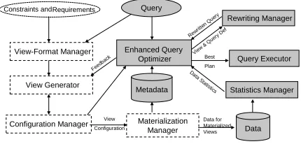
Data View Generator Enhanced Query Optimizer Materialization Manager Query Workload Constraints andRequirements Metadata Rewr
itten Q uery
Data S tatistics View Configuration Best Plan View & Q
uery Def Data for Materialized Views View-Format Manager Configuration Manager Rewriting Manager Statistics Manager Query Executor Feed back
Fig. 2.Designing derived data in QPET.
Enhanced Query Optimizer
Rewr itten Q
uery Data View Generator Materialization Manager Query Constraints andRequirements Metadata Data S
tatistics View Configuration Best Plan View & Q
uery Def Data for Materialized Views View-Format Manager Configuration Manager Rewriting Manager Statistics Manager Query Executor Feed back
Fig. 3.Using derived data in QPET.
can be assembled using, e.g., the query log [6].) We also assume that QPET has access to the relevant constraints on the outputs of the design stage, such as the amount of disk space available for storing the materialized views. Other things that can potentially be known in advance include requirements on possible rewritings of the workload queries using the views, such as, for instance, runtime ranges for the rewritings. Finally, for online redesign of materialized views, constraints on the amount of resources available for the design stage can be specified. (One direction of our current work is developing algorithms for designing derived data under hard resource constraints, with an emphasis on how the quality of the outputs depends on the values of the constraints.)
Using our QPET framework, data-management systems could design and materialize derived data by using specialized plug-and-play algorithms for each class of workload queries, such as star-schema queries. For this reason, each module active at the data-design stage uses algorithms that are appropriate for the given class of workload queries. In Section 4, we describe specific algorithms we use for workloads of aggregate queries under certain restrictions, in particular for queries on the star schema.10
In the design stage, the first thing to do is to delineate the search space of views that will be considered for materialization. This function is performed by theview-format manager, which determines the suggested format of views and rewritings and the related search space of candidate views based on the type of the workload queries and on other requirements. The view generator considers one by one the elements of the resulting search space of candidate views and passes those of the views that satisfy the input constraints (e.g., the given storage limit) on to the next module. Theconfiguration manager puts together some of the candidate views and tests the potential of the resulting view configurations to improve the evaluation performance of the workload queries. The tests are performed by an enhanced query optimizer, which estimates the costs of answering the workload queries using the configurations. (We use astatistics manager and the architecture of [6] to obtain query-cost estimates without materializing the views in the candidate configurations.) When obtaining query-cost estimates, the enhanced optimizer considers potential rewritings of the workload queries by calling arewriting manager, in the manner of [12].11
After a quality threshold is reached, typically after several iterations of designing and testing view configurations, thematerialization manager materializes the views in the best configuration as new stored data.
3.2 Using Derived Data in the QPET Framework
In Figure 3, shaded boxes with solid-line borders represent those modules in the QPET framework that are active at the stage of using derived data to answer customer queries. Suppose the system chooses to minimize the evaluation costs of a given query using the currently stored derived data. In this case, QPET first finds a “good” query plan while taking the materialized views into account, by using the enhanced query optimizer and rewriting manager in essentially the same way the modules are used in the view-design phase, see Section 3.1. (Depending on how appropriate the currently materialized views are for answering the query, the resulting query plan may or may not refer to stored view relations.) The resulting plan is
10
If the given query workload has queries that correspond to several distinct query classes such that a general solution would be too generic, one strategy to improve the quality of the solution could be to obtain separate specialized solutions for the sub-workloads according to the query classes, and then to try to merge some of the views, as proposed in, e.g., [6]. 11
passed to the query executor, which obtains an answer to the query in a standard way using the stored base or view relations.
Other than considering the stored derived data in generating query plans, using materialized views in QPET to answer a given query is not different from standard query processing. What can, however, make a difference in periodic online redesign of materialized views in our framework is which user queries are answered by taking the stored derived data into account. One approach could be to evaluate all user queries using the materialized views; the drawback here is the runtime penalty incurred by the optimizer for all input queries. As the currently materialized views were designed to improve the evaluation costs of some query workload that was fixed at the design stage, at the other extreme we could take the views into account only when evaluating those user queries that are part of that workload.12
Between the two extremes, multiple strategies are possible; those that we currently focus on in QPET make the decision for each query based on whether it could help characterize changes in the prevalent query workload over time. (For instance, QPET could use materialized views to evaluate frequent queries that are not in the fixed query workload. This way, the system can accumulate, for the future design stage, useful statistics on how the currently materialized views are used in answering important non-workload queries.) Other strategies are possible, based on which changes over time are tracked in the given data-management system; possible objects of interest include prevalent queries and stored data.
4 Complexity of the Problem and Parameterized Algorithm
We now discuss an approach we use within our QPET framework to improve the efficiency of evaluating aggregate queries without self-joins, by computing the queries using specially designed aggregate views. Recall that the BPUS approach of [7] evaluates aggregate star-schema queries using rewritings that have a materialized aggregate view as theonly relation in theFROM clause. Using the results in [10], we generalize the approach of [7] into an approach that uses oneor moreviews in each rewriting and that applies to amore general class of aggregate queries — queries that aggregate the same table, see Section 2 for a definition. In this framework, when looking for views that are potentially usable in computing given queries, we can examine all the views considered in [7], as well as additional views (with or without aggregation) that are defined on subsets of the set of relations in the FROM clause of the query. For instance, Examples 1 and 2 in Section 1 show an aggregate viewV1 that is defined on just the fact table Salesand that can be used, in joins with other relations, to evaluate aggregate queries Q1 throughQ3.
The idea of our approach is to extract, from a workload of queries that aggregate the same table, view templates, which serve as input queries to the view-selection algorithm that we use as a subroutine. (In our current implementation of QPET, this subroutine is the BPUS algorithm of [7].) The views returned by the subroutine are then materialized and used to automatically construct rewritings of the workload queries; the rewritings have one or more relations in their FROM clause and may or may not be aggregate queries. (That is, some of the rewritings of the given aggregate queries can be conjunctive querieswithout aggregation, see [10] for details and examples.) This approach can be tuned to explore different subspaces of the search space of views, depending on the input constraints such as the amount of system resources available for designing derived data.
4.1 Dealing with Inequality Comparisons
We first show how to obtain materialized views and rewritings for aggregate queries with inequality compar-isons with constants, including range-aggregate queries, without having to deal with the inequalities. (As shown in [24], in general the presence of inequalities increases the complexity of the problem of rewriting queries using views.) Recall that we consider only views without selection conditions, to maximize rewriting benefits for parameterized queries. Intuitively, we reduce the problem of designing and using materialized views for aggregate queries with inequalities to the problem for queries without inequalities, by allowing rewritings with inequalities. Theorem 1 says that the procedure results in correct processing of aggregate queries with inequality comparisons. More precisely, any set of views that is a solution for the modified queries without inequalities is also a solution for the original queries with inequalities.
12
Theorem 1. On a database D, let Q be a workload of select-project-join queries without self-joins and with aggregation sum,max,min, and count, such that at least one query inQ has inequality comparisons with constants. Let C be either a storage limit or a view-maintenance-cost constraint. By Q0 we denote
a workload of queries obtained by replacing inequality comparisons in Q with equalities on the same ar-guments. Consider a set V of select-project-join views with aggregation and without constants. If V is an admissible solution for a problem input (D,Q0
,C), thenV is also an admissible solution for a problem input (D,Q,C),assuming select-project-join rewritings with inequalities and with or without aggregation.13 4.2 View Selection: Sources of Exponentiality
We now observe that, as in the case of queries and views without aggregation [25], the view-selection problem for queries with aggregation has several sources of exponentiality, even under our restriction that materialized aggregate views do not have inequality comparisons or selection conditions. In our setting, the problem has four sources of exponentiality. First, even if we restrict ourselves to evaluating a single query using aggregate views, potentially useful views could be defined using subsetsor supersets of the relations in the query’s FROM clause. (Workloads of select-project-join queries with aggregation and self-joins might have useful aggregate views defined using exponentially more relations than used in any workload query [5, 10].) Second, useful views could be defined using various subsets of the join conditions in the query’sWHERE clause. Third, the set of grouping arguments in a useful view could be a superset of the query’s grouping arguments [7], or could even skip at least one grouping argument of the query [10]. The latter case holds for rewritings whose FROM clause has more than one relation, such as rewriting R1 in Example 1. (There exist central rewritings [10] in which the sets of grouping arguments of the aggregate view and of the query can even be disjoint.)
Finally, different queries in a query workload could use different aggregate functions (e.g., max and
sum) and could aggregate different arguments in base tables, as can be seen in, for instance, queries in the TPC-H benchmark [26]. In our approach we eliminate this source of exponentiality in view selection by having all views under consideration have all the aggregated arguments (i.e., all the combinations of the attribute to be aggregated with the aggregate function) that occur in the input query workload.
4.3 Complexity Results
We now show that for the practically important class of queries that aggregate the same table, two more of the four sources of exponentiality can be removed without removing any potentially useful aggregate views. The last result, Theorem 4, shows how removing yet another source of exponentiality that arises from varying subsets of relations in the FROM clauses of views, reduces the search space of views even further while preserving useful views. As a result, in our approach we need to deal with only one source of exponentiality, which arises from varying grouping arguments in the definitions of aggregate views. (All the results in this section hold for workloads of star-schema queries.)
We first establish that in evaluating workloads of aggregate queries without self-joins using materialized views, each optimal aggregate view can be defined using a low number of relations in theFROMclause. More precisely, the number of base relations in each view’sFROMclause is at most the number of relations used to define some workload query. Thus, for aggregate queries without self-joins, Theorem 2 removes the source of exponentiality in view selection that comes from varying, in view definitions, up to exponentially-sized combinations of relations in the FROM clauses of the input queries. As a result (Corollary 1), the problem has lower complexity for this class of queries, NP-complete rather than exponential-time lower bound.
Theorem 2. (Restricted definitions of useful central views) On a databaseD, letQbe a workload of select-project-join queries without self-joins and with aggregation sum, max, min, and count. Let the aggregated arguments of all the queries come from a single base table in D. LetV be an optimal set of central aggregate views for a problem input (D,Q,C), whereC is a storage limit or a view-maintenance-cost constraint. Then each view in V can be defined using a subset of the FROM clause of some query Q Q.
Corollary 1. For problem inputs as Theorem 2, the view-selection problem is NP-complete.
13
The next result, Theorem 3, holds for query workloads that additionally have the same join conditions (see Section 2). Intuitively, under this restriction we can generate all useful central aggregate views by combining all meaningful subsets of the FROM clause of the input queries (each such subset determines all join conditions in the WHERE clause) with all possible sets of useful grouping arguments. That is, the same-join condition removes the source of exponentiality that comes from varying join conditions in the WHEREclauses of the views.
Theorem 3. (Restricted search space of central views) For problem inputs as in Theorem 2, and if the queries in the workload Q additionally have the same join conditions, then the search space of optimal central aggregate views is at most doubly exponential in the size of the input query workload Q.
Thus, for workloads of aggregate queries that have the same join conditions we need to deal with just two sources of exponentiality in view definitions instead of the four that are discussed in Section 4.2.
So far, we have shown that for a practically important class of aggregate queries, some of the sources of exponentiality (Section 4.2) can be removed without removingany potentially useful views from consider-ation. Our last result in this section says that focusing on a certain important subclass of views (views that all share the sameFROM clause) removes an additional exponent from the complexity of the view-selection problem.14
Theorem 4. For problem inputs as in Theorem 3, and if in addition all views under consideration have the same FROMclause, then the search space of optimal central aggregate views is at most singly exponential in the size of the input query workload Q.
We will see in Section 4.4 how this restriction to views that share the sameFROM clause allows us to use a view-selection method for just star-schema queries (such as BPUS [7]) as a subroutine in our approach to view selection for amore generalclass of queries that aggregate the same table, such as the query workload of Example 2 in Section 1.
4.4 Outline of the Algorithm
We now discuss our parameterized algorithm for selecting and using aggregate views to reduce the eval-uation costs of workloads of aggregate queries. Suppose we are given a database D and a workload Q of aggregate select-project-join queries that aggregate the same table, for instance the fact table in the star-schema setting. In addition, we are given (1) a constraint C1 on the runtime of the view-design algorithm,
and (2) a constraint C2 on the materialized views — either a storage limit or a view-maintenance-cost
constraint. To reduce the costs of evaluating the workloadQonDunder the constraintC2, we select, under
the time constraintC1, views with aggregation (all the views will share the sameFROMclause) and construct
rewritings of the queries using the views as follows:
AlgorithmComposite-Aggregate-Rewritings(databaseD, query workloadQ, constraintsC1 andC2). Output: setRof rewritings ofQusing aggregate viewsV.
1 Begin
2 Initialize ˆQ,Rto empty sets;
3 F :=Nonempty-Overlap(Q,C1); /* Set F to relations that occur in all queries in Q */ /* (1) */
4 /* Determine input queries Qˆ to the Lattice-Select-Views subroutine: */ /* (2) */
5 For each queryQ Qdo: Begin Qˆ :=Input-Lattice-Select(Q,F); ˆQ := ˆQ ∪ {Qˆ}; End
6 /* Collect into a set A the aggregated arguments in all the queries in Q */ /* (3) */
7 V :=Lattice-Select-Views({Qˆ,F,D,C2,A); /* Generate central aggregate views V */ /* (4) */
8 /* Construct rewritings R of the queries in Q using the aggregate views V: */ /* (5) */
9 For each queryQ Qdo: Begin R :=Build-Rewriting(Q,V,F);R := R ∪R; End 10 OutputR;
11 End.
14
Conceptually, the algorithm finds central aggregate views V for the queries Q using a view-selection algorithm for star-schema queries (such as BPUS [7]) as a subroutine Lattice-Select-Views, see step(4), and then uses the views V to build equivalent rewritings R of the queries Q. In the rewritings R, the viewsV “cover” all or somesubgoals of the queries: In each rewriting,F are the subgoals “covered” by a view from V. As the size of the set F determines the runtime of the view-design subroutine of step(4), lower values of the design-time constraintC1 result in choosing smaller setsF, see step (1). In the overall
algorithm (steps(1)through(5)), the subroutines for generating input queries ˆQforLattice-Select-Views, step (2), and for constructing the rewritings R of Q, step (5), ensure the equivalence of the rewritings to the queries, while Lattice-Select-Views, step (4), produces views V that are guaranteed to reduce the evaluation costs w.r.t. the subgoals F in each query on the database D, subject to the constaint C2.
Theorem 5. Algorithm Composite-Aggregate-Rewritings is sound for problem inputs as in Theorem 2 whenever all the queries in the workload Q have the same join condition w.r.t. the setF.15
That is, in this case the algorithm returns equivalent rewritings of the queries in Q using central aggregate views.
Different choices of the FROM clause F of the views determine different search spaces of views with aggregation for the input query workload. (For each such choice, note the performance guarantees of the algorithm induced by the use of theLattice-Select-Views subroutine, e.g., BPUS of [7], in case the algorithm is applied to queries on the star schema with the associated integrity constraints.) Varying the value of the overlap set F results in different degrees of “goodness” of the output of the algorithm Composite-Aggregate-Rewritings along several metrics: As the number of base relations inF increases,
– the evaluation costs of the workload queries Q using the output rewritings Rtend to decrease;
– the runtime of the Lattice-Select-Views subroutine tends to increase;
– the total size (and thus disk-space requirement) for the output materialized views V tends to increase;
– the total maintenance costs for the output materialized views V tend to increase.
Intuitively, all these trends are caused by the “degree of coverage” of the evaluation plans for the workload queries by the evaluation plans for the views. (The sizes of evaluation plans for the views are determined by the number of base relations in the definitions of the viewsV.) As an illustration, view V1in Example 1 has just theSalestable in its FROMclause and thus “covers less” of the queryQ1 than the viewV2, which is defined using tables Salesand Customer.
5 Implementation and Preliminary Experimental Evaluation
Our implementation of the QPET framework is written in C and is based on an open-source relational data-management system PostgreSQL [27] version 7.3.4. The current version of QPET is available on-line [4]; it incorporates support for answering SQL queries using materialized views, as described in [12], and for generating aggregate views using the BPUS algorithm of [7]. Implementing other view-generation algorithms, including that of [9], and implementing automated evaluation of arbitrary select-project-join queries with aggregation using materialized views and indexes [8] is part of our ongoing work.
Region Nation2 Nation1 Orders Customer PartSupp Supplier Part Lineitem
396 2,103 2,103 482,877,440 244,883,456 5,830,541 14,188,544 1,193,906 2,147,483,647 Size (bytes) Name
TPC-H Tables
Fig. 4. Sizes of base TPC-H tables (in bytes).
We have conducted preliminary experiments to evaluate the system archi-tecture and techniques presented in Sections 3 and 4. All experiments were run on a machine with a 2.8GHz Intel P4 processor, 512MB RAM, and an internal 80GB hard drive running Linux RedHat 9 with kernel version 2.4.20-8 and our implementation of QPET [4]. The experimental results show the following. (1) Using materialized views designed by our approach results in query runtimes comparable to runtimes of the queries using views output by the BPUS algo-rithm, which we used for comparison purposes. (2) Disk-space requirements for storing materialized views in our approach are acceptable, compared to the re-quirements for storing views produced by BPUS. (In addition, by design of views in our approach, the view relations require less system resources for maintenance
15
than the relations for BPUS views, see Section 4.4.) (3) Finally, the time required to design views in our approach can be drastically lower than the time required to design BPUS views for the same queries.
We give here just a brief summary of the experiments; a detailed account of the experimental setup and results can be found in Appendix B. The goal of the experiments was to compare evaluation costs for a workload of aggregate star-schema queries in three settings:
– using just the stored relations in the original database;
– using materialized views obtained by our approach; and
– using materialized views obtained by an approach in the literature.
922,962,047 5008 43,995,526 17 505 10 77,529,577 3074 192,158,348 39 752,916 9 761,573,474 7936 192,158,348 39 3 8 127,090,353 6496 219,496,362 101 1 7 1,461,958 120 1,461,958 120 1 6 4,938,267 6656 141,452,410 5 5 5 410,344,447 5105 199,699,334 113 1,281 3 121,758 112 121,758 112 1 1 View Size View ID View Size View ID Rows Returned
Query ID Fact-Table Views Used BPUS Views Used
Fig. 5.Answer sizes for workload queries and views; view sizes are in bytes. Fact-table views are the same forQ8 and Q9. As an approach in the literature, we chose the BPUS
al-gorithm of [7] because it gives strong performance guarantees when applied to a wide range of types of view lattices. (The approach of [9] achieves the same guarantees as BPUS for a more restricted set of view lattices.) For our approach in the experiments, we chose to design and materializefact-table views, that is, views whoseFROMclause has just the fact table in the star schema. Recall that query rewritings with fact-table views have at least as many joins as rewritings of the same query using other view types, and are thus the “least efficient” rewritings in our approach. Thus, by choosing
fact-table views for the experiments, we were interested in seeing how much worse query-evaluation costs can be when using our approach than when using the BPUS approach. In the remainder of this section, by “BPUS views or rewritings” (“fact-table views or rewritings,” respectively) we refer to the views or rewritings based on the BPUS approach (based on our approach, respectively).
We did the experiments on a TPC-H database benchmark [26]; the sizes of the stored tables are shown in Figure 4. (We used the scale factor of one for the stored data.) The query workload for the experiments had eight aggregate queries, with between one and eight tables in the FROM clause and with aggregation on the Lineitemtable, which is the fact table in the experiments.16
The queries can be used as an input to the BPUS algorithm because the referential-integrity constraints on the stored TPC-H data guarantee that the views produced by BPUS, with all eight tables in the FROM clause, can be used to equivalently rewrite even those queries whose FROMclause has fewer tables.
BPUS Lattice
Fact-Table Lattice 40 128
Number of Nodes In the Lattice
1,920 8,192
Time to Generate Views (seconds)
Fig. 6. View-generation runtimes and lat-tice sizes, for fact-table and BPUS views. We used the BPUS algorithm to design views for both
fact-table rewritings (as a subroutine in our algorithm, see Section 4.4) and BPUS rewritings of the workload queries. In both cases, size estimates for relations in the view lat-tices were obtained by running the queries for all possible lattice views on TPC-H stored data with scale factor of 0.1
and by extrapolating the sizes of the answers to the queries to the size of the stored data used to evaluate the workload queries and their rewritings.
0 20 40 60 80 100 120 140 160
1 3 5 6 7 8 10
Query ID T im e i n m il li s e c o n d s No Views Fact- Table Views BPUS Views
Fig. 7. Runtimes of the workload queries. To design views for BPUS rewritings of the workload
queries, we ran the BPUS algorithms using the workload queries as inputs. As explained in Section 4, in our ap-proach the FROM clause of the views we design determines automatically the rewriting of each querybefore we design the actual views. (The BPUS approach also determines the rewritings automatically based on which views can be used to evaluate the input queries.) Thus, once we settled on fact-table views for the rewritings in our approach, the rewritings we obtained determined automatically the in-put queries to the BPUS subroutine, which then designed
16
fact-table views for the workload. Note that by design of BPUS, in each case we obtained a set of views for the entire query workload, rather than for its individual queries. In addition, recall that by design of BPUS, views produced by the algorithm have no comparisons with constants and can thus be used to evaluate any instantiation of theparameterized versions of the workload queries.
The fact-table and BPUS rewritings of the workload queries determined view lattices in the BPUS algorithm for seven and thirteen grouping attributes respectively. (The grouping arguments in a view lattice are a union of the grouping arguments of all the input queries for BPUS.) Figure 6 shows the number of nodes in view lattices and the runtimes for BPUS when called to generate views for fact-table rewritings and for BPUS rewritings. Increasing the number of tables in the FROM clause of views in our approach would tend to cause an increase in the number of required output arguments in the views. (These required arguments include those attributes of the tables in each view’s FROM clause that participate in join and selection conditions in the rewritings, as well as those attributes of the tables in the FROM clause that are grouping arguments of the query.) Accordingly, the size of the view lattice explored by the BPUS subroutine would tend to increase exponentially with each table added to theFROMclause of views designed in our approach. The reason is, the size of a view lattice in the BPUS algorithm is exponential in the number of grouping attributes in the algorithm input.
Figure 5 has information on views produced by the BPUS subroutine for fact-table rewritings (seven views; note that the same view was produced for queriesQ8andQ9) and for BPUS rewritings (eight views) for our query workload. Intuitively, storing materialized fact-table views should require more disk space than storing BPUS views, because a grouping argument of a fact-table view is akeyargument of a dimension table whenever the corresponding grouping argument of a BPUS view (for the same workload query) is a nonkey argument of the same dimension table. When the views were materialized on the database for the experiments, storing the relations for the fact-table views did not require significantly more disk space than storing the relations for the BPUS views.
As discussed in Section 4, once the view-design subroutine returns aggregate views in our approach, the most appropriate materialized views (i.e., views that have a minimal-size relation among the views that have all the required grouping arguments for the rewriting) are selected automatically into query rewritings that were designed before calling the subroutine. Similarly, selecting the most appropriate views to rewrite workload queries is straightforward in the BPUS approach, which we use for comparison in the experiments. (In fact, building rewritings in the BPUS approach is a special case of building rewritings in our approach.)
rewritings of the range-aggregate queries are comparable with the runtimes of the rewritings (both fact-table and BPUS) of the corresponding point queries and are significantly lower than the runtimes of the queries when evaluated without views.
Acknowledgments
We are grateful to Kyoung-hwa Kim and Simran Sandhu who have been part of the implementation team.
References
1. Shasha, D., Bonnet, P. Database Tuning: Principles, Experiments, and Troubleshooting Techniques. Morgan Kaufmann (2002)http://www.distlab.dk/dbtune/.
2. Microsoft Research AutoAdmin Project: Self-Tuning and Self-Administering Databases. (http://research.microsoft. com/dmx/autoadmin/default.asp)
3. IBM Autonomic Computing. (http://www.research.ibm.com/autonomic/)
4. Chirkova, R., Gupta, S., Kim, K.H., Sandhu, S. Extensible framework for query-performance enhancement by tuning. Code downloads and documentation are available fromhttp://research.csc.ncsu.edu/selftune/(2004)
5. Chirkova, R., Halevy, A., Suciu, D. A formal perspective on the view selection problem. VLDB Journal11(2002) 216–237 6. Agrawal, S., Chaudhuri, S., Narasayya, V. Automated selection of materialized views and indexes in SQL databases. In:
Proceedings of VLDB (2000) 496–505
7. Harinarayan, V., Rajaraman, A., Ullman, J. Implementing data cubes efficiently. In: Proc. SIGMOD (1996) 205–216 8. Gupta, H., Harinarayan, V., Rajaraman, A., Ullman, J. Index selection for OLAP. In: Proceedings of ICDE (1997) 208–219 9. Shukla, A., Deshpande, P., Naughton, J. Materialized view selection for multidimensional datasets. In: Proceedings of
VLDB (1998) 488–499
10. Afrati, F., Chirkova, R. Selecting and using views to compute aggregate queries. Submitted for publication; earlier version available athttp://dbgroup.ncsu.edu/aggregAquv.pdf(2004)
11. Halevy, A.Y. Answering queries using views: A survey. VLDB Journal10(2001) 270–294
12. Chaudhuri, S., Krishnamurthy, R., Potamianos, S., Shim, K. Optimizing queries with materialized views. In: Proceedings of the Eleventh International Conference on Data Engineering (ICDE) (1995) 190–200
13. Chaudhuri, S., Narasayya, V. AutoAdmin ’What-if’ index analysis utility. In: Proc. SIGMOD (1998) 367–378
14. Agrawal, S., Chaudhuri, S., Narasayya, V. Materialized view and index selection tool for Microsoft SQL Server 2000. In: Proceedings of ACM SIGMOD (2001)
15. Widom, J. Research problems in data warehousing. In: Proceedings of CIKM (1995)
16. Gray, J., Chaudhuri, S., Bosworth, A., Layman, A., Reichart, D., Venkatrao, M. Data cube: A relational aggregation operator generalizing Group-by, Cross-Tab, and Sub Totals. Data Mining and Knowledge Discovery1(1997) 29–53 17. Chaudhuri, S., Dayal, U. An overview of data warehousing and OLAP technology. SIGMOD Record26(1997) 65–74 18. Agarwal, S., Agrawal, R., Deshpande, P., Gupta, A., Naughton, J., Ramakrishnan, R., Sarawagi, S. On the computation
of multidimensional aggregates. In: Proceedings of VLDB (1996) 506–521
19. Gupta, A., Harinarayan, V., Quass, D. Aggregate-query processing in data warehousing environments. In: Proceedings of VLDB (1995) 358–369
20. Srivastava, D., Dar, S., Jagadish, H., Levy, A. Answering queries with aggregation using views. In: Proc. VLDB (1996) 318–329
21. Cohen, S., Nutt, W., Serebrenik, A. Rewriting aggregate queries using views. In: Proceedings of PODS (1999) 155–166 22. Chaudhuri, S., Narasayya, V. An efficient cost-driven index selection tool for Microsoft SQL server. In: Proceedings of
VLDB (1997) 146–155
23. Kimball, R., Ross, M. The Data Warehouse Toolkit (second edition). Wiley Computer Publishing (2002)
24. Afrati, F., Li, C., Mitra, P. Answering queries using views with arithmetic comparisons. In: Proc. PODS (2002) 209–220 25. Levy, A., Mendelzon, A., Sagiv, Y., Srivastava, D. Answering queries using views. In: Proceedings of PODS (1995) 95–104 26. TPC-H: TPC Benchmark H (Decision Support). (Available fromhttp://www.tpc.org/tpch/spec/tpch2.1.0.pdf) 27. PostgreSQL (Open source database-management system)http://www.postgresql.org/.
28. TPC-H (TPC Benchmark H (Decision Support).) Available fromhttp://www.tpc.org/tpch/ spec/tpch2.1.0.pdf.
A Example: Materialized Views Explored by the BPUS Algorithm of [7]
This example shows the format of materialized views explored by the greedy algorithm BPUS of [7] for the query workload{ Q1, Q2 } in Example 1 of Section 1.
W1: SELECT c.CustID AS CID1, Year, Month, W2: SELECT t.Year AS Year2, State, SUM(QuantitySold) AS SQS1 SUM(QuantitySold) AS SQS2 FROM Sales s, Time t, Customer c FROM Sales s, Time t, Customer c WHERE s.DateID = t.DateID WHERE s.DateID = t.DateID
AND s.CustID = c.CustID AND s.CustID = c.CustID
GROUP BY c.CustID, Year, Month; GROUP BY t.Year, State;
QueryQ1(Q2, respectively) can be answered using selection, grouping, and aggregation on the viewW1 (W2, respectively). Finding the grouping arguments of the viewsW1andW2using BPUS requires considering all subsets of the set of four attributes { CustID, Year, Month, State } of the stored tables.
Another BPUS solution for the workload { Q1, Q2 } could comprise a single aggregate view, W. For instance, query Q1could be evaluated using this rewriting R:
R: SELECT CustID, CustName,Addr, sum(SumQS)
FROM W WHERE Year = 2004 AND Month >= 4 AND Month <= 6 GROUP BY CustID, CustName, Addr;
That is, suppose we have a materialized aggregate view W that has all “necessary” arguments; we will elaborate shortly on which arguments are necessary in W for evaluating Q1 and Q2. Let W have an attribute SumQSwhose value is the sum ofQuantitySold(see the schema ofSalesin Example 1) for each combination of the grouping arguments of W. Then the answer toQ1 is computed using the rewritingRby doing Q1’s grouping and aggregation on those rows in the answer to W that satisfy the conditions Year = 2004 AND Month >= 4 AND Month <= 6. The answer toQ2 could be computed usingWin a similar way.
Here is one possible definition forW:
W: SELECT s.CustID, Year, Month, State, SUM(QuantitySold) AS SumQS FROM Sales s, Time t, Customer c
WHERE s.DateID = t.DateID AND s.CustID = c.CustID GROUP BY s.CustID, Year, Month, State;
That is, Wreturns total sales per customer ID, year, month, and customer state.
BPUS [7] considers all sets of views — including { W1, W2 } and { W } — that (1) can be used to evaluate the queryQ1using the rewriting Rabove, and (2) can be used to evaluate the queryQ2using the same approach. All such sets W of views need to satisfy several requirements. First, each view in the set of viewsW “covers” the body of each workload query, by using all the relations in theFROM clause and all the join conditions of each query. Second, for each workload query, at least one view inW needs to have in its GROUP BYclause at least all the grouping arguments of the query and the arguments in all the query’s selection conditions. (In this sense, the above SQL definition of Wis “minimal” for the queries Q1 and Q2, because all the arguments in theSELECTclause ofWare used in rewritings of the two queries.) Finally, each view in W should have an attribute (SumQS in our example) whose value is the result of aggregating the selected argument (QuantitySoldin our example) for each combination of the grouping arguments of the view.
B Experimental Setup and Results
We have used the TPC-H [28] database with scale factor of one and a query workload based on TPC-H queries.
B.1 The Modified TPC-H Schema
The only modification of the schema concerns the Nationtable: To create a workload of queries without self-joins (i.e., without duplicate occurrences of the same table in the FROM clause), we used two copies of the Nationtable, named Nation1 and Nation2. In addition, we do not show here the schema of the Partsupprelation, as Partsuppis not in definitions of the queries we used to define our query workload.
Part(PARTKEY,NAME,MFGR,BRAND,TYPE,SIZE,CONTAINER,RETAILPRICE,COMMENT) Table size: ScaleFactor ×200,000
Supplier(SUPPKEY,NAME,ADDRESS,NATIONKEY,PHONE,ACCTBAL,COMMENT) Table size: ScaleFactor ×10,000
Customer(CUSTKEY,NAME,ADDRESS,NATIONKEY,PHONE,ACCTBAL,MKTSEGMENT,COMMENT) Table size: ScaleFactor ×150,000
Nation1(NATIONKEY,NAME,REGIONKEY,COMMENT) Table size: 25
Nation2(NATIONKEY,NAME,REGIONKEY,COMMENT) Table size: 25
Lineitem(ORDERKEY,PARTKEY,SUPPKEY,LINENUMBER,QUANTITY,
EXTENDEDPRICE,DISCOUNT,TAX,RETURNFLAG,LINESTATUS,SHIPDATE, COMMITDATE,RECEIPTDATE,SHIPINSTRUCT,SHIPMODE,COMMENT) Table size: ScaleFactor ×6,000,000
Orders(ORDERKEY,CUSTKEY,ORDERSTATUS,TOTALPRICE,ORDERDATE, ORDERPRIORITY,CLERK,SHIPPRIORITY,COMMENT)
Table size: ScaleFactor ×1,500,000
Region(REGIONKEY,NAME,COMMENT) Table size: 5
Referential-integrity constraints on the schema:
From Lineitem(PARTKEY) to Part(PARTKEY) From Lineitem(SUPPKEY) to Supplier(SUPPKEY) From Customer(NATIONKEY) to Nation2(NATIONKEY) From Supplier(NATIONKEY) to Nation1(NATIONKEY) From Nation2(REGIONKEY) to Region(REGIONKEY) From Orders(CUSTKEY) to Customer(CUSTKEY) From Lineitem(ORDERKEY) to Orders(ORDERKEY)
B.2 The Product-of-Dimensions Views
For the experiments, each product-of-dimensions (POD) view is defined as follows:
– the FROMand WHEREclauses of the query represent a join of all the relations in Section B.1, as given in queries in [28];
– for each query, theGROUP BYandSELECTclauses of the query is as specified (in Datalog) in Section B.3.
B.3 The Query Workload: Modified TPC-H Queries
In this section, the IDs of the modified queries are the IDs of the corresponding original TPC-H queries in [28]. In the experiments, all the placeholders for constants in the queries below were replaced by constant values occurring in the TPC stored data. The query workload for the experiments consists of the modified queriesQ1, Q3, Q5, Q6, Q7, Q8, Q9, Q10.
Pricing Summary Report Query (Q1)
1. Objective: Reports the amount of business that was billed, shipped, and returned. 2. Modified query Q1 for the experiments, in SQL:
SELECT
l_returnflag, l_linestatus,
SUM(l_extendedprice), COUNT(*)
FROM
lineitem WHERE
l_shipdate = date ‘[DATE]’ GROUP BY
l_returnflag, l_linestatus;
3. Modified query Q1 for the experiments, in Datalog:
q1(RF, LS, sum(EX), count)
:-L(OK, P K, SK, LN, QT, EX, DS, T X, RF, LS,‘date0, CD, RD, SI, SM, C8).
4. Input for product-of-dimensions lattice:
qP
1(RF, LS, SD)
That is, to be answered using the outputs of the BPUS algorithm of [7] on the product-of-dimensions lat-tice, this query needs a view whose grouping arguments include argumentsReturnflag, Linestatus, and Shipdateof the relation Lineitem.
In general, the rule for formingqP
i for a queryqi is as follows: take all grouping arguments ofqi and all
the arguments of qi that are involved in (in)equality comparisons with constants.
5. Definition of product-of-dimension view for the query: on prodOfDims, see Section B.2. In SQL:
SELECT returnflag, linestatus, shipdate,
SUM(extendedprice) AS sumex, count(*) AS totalcount INTO _0112
FROM prodOfDims
GROUP BY returnflag, linestatus, shipdate;
In Datalog:
V0112(RF, LS, SD, sum(EX), count(∗)) :−
prodOf Dims.
6. Rewriting of the query using the product-of-dimension view: In SQL:
SELECT returnflag, linestatus, SUM(sumex), SUM(totalcount) AS count FROM _0112
WHERE shipdate = date ’1998-12-01’ GROUP BY returnflag, linestatus;
In Datalog:
Q1(RF, LS, SU M(sumex), SU M(totalcount)) :−
V0112(RF, LS,0
1998−12−010, sumex, totalcount
7. Input for fact-table lattice17
:
qF
1(RF, LS, SD)
That is, to be answered using the outputs of the BPUS algorithm of [7] on the fact-table lattice, this query needs a view whose grouping arguments include arguments Returnflag, Linestatus,and Shipdate of the relation Lineitem. (Inputs qP
1 and q
F
1 are the same because the body of q1 has just
one table. See below that whenever the body of a query has at least two tables,qP andqF for the query will be different.)
In general, the rule for formingqF
i for a queryqi is as follows: take all argumentsAofLineitem(in the
body of the query qi), such that: (1) A is a grouping argument in the head ofqi, or (2) A is involved
in (in)equality comparisons with constants in the body of qi, or (3) A is needed for joins with other
relations in the body ofqi.
8. Definition of fact-table view for the query: In SQL:
SELECT returnflag, linestatus, shipdate,
SUM(extendedprice) AS sumex, count(*) AS totalcount INTO _112
FROM lineitem
GROUP BY returnflag, linestatus, shipdate;
In Datalog:
V112(RF, LS, SD, sum(EX), count(∗)) :−
L(OK, P K, SK, LN, QT, EX, DS, T X, RF, LS, SD, CD, RD, SI, SM, C8).
9. Rewriting of the query using the fact-table view: In SQL:
SELECT returnflag, linestatus, SUM(sumex), SUM(totalcount) AS count FROM _112
WHERE shipdate = date ’1998-12-01’ GROUP BY returnflag, linestatus;
In Datalog:
Q1(RF, LS, SU M(sumex), SU M(totalcount)) :−
V112(RF, LS,0
1998−12−010, sumex, totalcount
).
Shipping Priority Query (Q3)
1. Objective: Retrieves the ten unshipped orders with the highest value. 2. Modified query Q3 for the experiments, in SQL:
SELECT
l_orderkey,
sum(l_extendedprice), o_orderdate,
o_shippriority FROM
customer, orders, lineitem
17
WHERE
l_returnflag = ‘[RETURNFLAG]’ AND c_custkey = o_custkey AND l_orderkey = o_orderkey AND l_shipdate = date ‘[DATE]’ GROUP BY
l_orderkey, o_orderdate, o_shippriority;
3. Modified query Q3 for the experiments, in Datalog:
q3(OK, OD, SP, sum(EX))
:-C(CK, N4, A4, N K, P4, B4, M S, C4),
O(OK, CK, OS, T R, OD, OP, CL, SP, C7),
L(OK, P K, SK, LN, QT, EX, DS, T X,‘r0, LS,‘date0, CD, RD, SI, SM, C8).
4. Input for product-of-dimensions lattice:
qP
3(OK, OD, SP, SD, RF)
5. Definition of product-of-dimension view for the query: on prodOfDims, see Section B.2. In SQL:
SELECT orderkey, returnflag, linestatus, shipdate,
custkey, mktsegment, nationkey2, orderdate, shippriority, regionkey, SUM(extendedprice) AS sumex, count(*) AS totalcount INTO _5105
FROM prodOfDims
GROUP BY orderkey, returnflag, linestatus, shipdate, custkey, mktsegment, nationkey2, orderdate, shippriority, regionkey;
In Datalog:
V5105(OK, RF, LS, SD, CK, M S, N K2, OD, SP, RK, SU M(ex), count(∗)) :−
prodOf Dims.
6. Rewriting of the query using the product-of-dimension view: In SQL:
SELECT orderkey, SUM(sumex), orderdate, shippriority FROM _5105
WHERE returnflag = ’R’ AND shipdate = ’1995-04-16’
GROUP BY orderkey, orderdate, shippriority;
In Datalog:
Q3(OK, SU M(sumex), OD, SP) :−
V5105(OK,0R0, LS,01995−04−160, CK, M S, N K2, OD, SP, RK, SU M EX, totalcount).
7. Input for fact-table lattice:
qF
3(OK, SD, RF)
SELECT orderkey, returnflag, linestatus, shipdate, SUM(extendedprice) AS sumex, count(*) AS totalcount INTO _113
FROM lineitem
GROUP BY orderkey, returnflag, linestatus, shipdate;
In Datalog:
V113(OK, RF, LS, SD, SU M(ex), COU N T(∗)) :−
L(OK, P K, SK, LN, QT, EX, DS, T X, RF, LS, SD, CD, RD, SI, SM, C8).
9. Rewriting of the query using the fact-table view: In SQL:
SELECT l.orderkey, SUM(sumex), orderdate, shippriority FROM customer c, orders o, _113 l
WHERE returnflag = ’R’ AND o.custkey = c.custkey AND l.orderkey = o.orderkey AND shipdate = date ’1995-04-16’
GROUP BY l.orderkey, orderdate, shippriority;
In Datalog:
Q3(OK, SU M(sumex), OD, SP) :−
V113(OK,0R0, LS,01995−04−160
, sumex, totalcount),
C(CK, N4, A4, N K, P4, B4, M S, C4), O(OK, CK, OS, T R, OD, OP, CL, SP, C7).
Local Supplier Volume Query (Q5)
1. Objective: Lists the revenue volume done through local suppliers. 2. Modified query Q5 for the experiments, in SQL:
SELECT
n_name,
SUM(l_extendedprice) FROM
customer, orders, lineitem, supplier, nation1, region WHERE
c_custkey = o_custkey
AND l_orderkey = o_orderkey AND l_suppkey = s_suppkey AND s_nationkey = n_nationkey AND n_regionkey = r_regionkey AND r_name = ‘[REGION]’
AND o_orderdate = date ‘[DATE]’ GROUP BY
n_name;
q5(N51, sum(EX))
:-C(CK, N4, A4, N K2, P4, B4, M S, C4),
O(OK, CK, OS, T R,‘date0, OP, CL, SP, C7),
L(OK, P K, SK, LN, QT, EX, DS, T X, RF, LS, SD, CD, RD, SI, SM, C8),
S(SK, N2, A2, N K1, P2, B2, C2),
N at1(N K1, N51, RK, C51),
R(RK,‘region0, C
6).
4. Input for product-of-dimensions lattice:
qP
5(N51, OD, N6)
5. Definition of product-of-dimension view for the query: on prodOfDims, see Section B.2. In SQL:
SELECT orderdate, nationkey1, n1_name, regionkey, name, SUM(extendedprice) AS sumex, count(*) AS totalcount INTO _6656
FROM prodOfDims
GROUP BY orderdate, nationkey1, n1_name, regionkey, name
In Datalog:
V6656(OD, N K1, N1.name, RK, R.name, SU M(ex), count(∗)) :−
prodOf Dims.
6. Rewriting of the query using the product-of-dimension view: In SQL:
SELECT n1_name, SUM(sumex) FROM _6656
WHERE name=’AFRICA’
AND orderdate= ’1993-07-01’ GROUP BY n1_name;
In Datalog:
Q5(N1.name, SU M(sumex)) :−
V6656(0
1993−07−010, N K
1, N1.name, RK,0AF RICA0, SU M EX, totalcount
).
7. Input for fact-table lattice:
qF5(OK, SK)
8. Definition of fact-table view for the query: In SQL:
SELECT orderkey, suppkey, SUM(extendedprice) AS sumex, count(*) AS totalcount INTO _005
FROM lineitem
GROUP BY orderkey, suppkey;
In Datalog:
V5(OK, SK, SU M(EX), count(∗)) :−
L(OK, P K, SK, LN, QT, EX, DS, T X, RF, LS, SD, CD, RD, SI, SM, C8).
![Fig. 1. Overall system architecture [6, 14].](https://thumb-us.123doks.com/thumbv2/123dok_us/1331321.1166080/6.612.380.549.454.615/fig-overall-system-architecture.webp)