Develop Methods To Evaluate the Performance of Aflatoxin Sampling Plans for Shelled Corn.

(1)

ABSTRACT

JOHANSSON, ANDERS STURE. Develop Methods To Evaluate the Performance of

Aflatoxin Sampling Plans for Shelled Corn. (Under the direction of Thomas Burton

Whitaker.)

Eighteen lots of shelled corn were tested for aflatoxin contamination. The

variability and distributional characteristics associated with the aflatoxin testing

procedure were investigated. The total variance associated with testing shelled corn was

estimated and partitioned into sampling, sample preparation, and analytical variances.

All variances were found to increase with an increase in aflatoxin concentration. Using

regression analysis, mathematical expressions were developed to model the relationship

between aflatoxin concentration and the total, sampling, sample preparation, and

analytical variances. The expressions for these relationships were used to estimate the

variance for any sample size, subsample size, and number of analyses for a specific

aflatoxin concentration. For example, testing a lot with 20 parts per billion (ppb)

aflatoxin using a 2.5 lb sample, Romer mill and 50 g subsample, and HPLC analysis, the

total, sampling, sample preparation, and analytical variances are 274.9 (CV=82.9%),

214.0 (CV=73.1%), 56.3 (CV=37.5%), and 4.6 (CV=10.7%), respectively. The

percentage of the total variance for sampling, sample preparation, and analytical is 77.8,

20.5, and 1.7 %, respectively.

Next, fifteen positively skewed distributions were each fitted to 18 empirical

distributions of aflatoxin test results for shelled corn. The compound gamma distribution

was selected to model the sample aflatoxin test results for shelled corn. The method of

moments technique was chosen to estimate the parameters of the compound gamma

(2)

compound gamma distribution for any lot aflatoxin concentration and test procedure.

Observed acceptance probabilities were compared to operating characteristic curves

predicted from the compound gamma distribution and all 18 distributions of sample

aflatoxin test results were found to lie within a 95% confidence band.

Using the mean and variance relationships to compute the parameters of the

compound gamma distribution, 16 sampling plans, based on four sample sizes and four

sample acceptance levels were created and analyzed. For a given sample size, decreasing

the sample acceptance level, using a sample acceptance level equal to the regulatory

guideline: (a) decreases the percentage of lots accepted while increasing the percentage

of lots rejected at all aflatoxin concentrations; (b) increases misclassification of lots

(both false positives and false negatives) while decreasing the percentage of correct

decisions; and (c) decreases the average aflatoxin concentration in the lots accepted and

lots rejected. For a given sample size where the sample acceptance level is less than the

regulatory guideline, the number of false positives increases and the number of false

negatives decreases when compared to the situation where the sample acceptance level

equals the regulatory guideline. For a given sample size, where the sample acceptance

level is greater than the regulatory guideline, the number of false positives decreases and

the number of false negatives increases when compared to the situation where the sample

acceptance level equals the regulatory guideline. Increasing the sample size for a given

sample acceptance level, where the legal limit equals the sample acceptance level: (a)

increases the percentage of lots accepted at lower concentrations while increasing the

(3)

decisions; and (c) decreases the average aflatoxin concentration in the lots accepted while

(4)

DEVELOP METHODS TO EVALUATE THE PERFORMANCE OF

AFLATOXIN SAMPLING PLANS FOR SHELLED CORN

by

ANDERS STURE JOHANSSON

A dissertation submitted to the Graduate Faculty of North Carolina State University

in partial fulfillment of the requirements for the Degree of

Doctor of Philosophy

BIOLOGICAL AND AGRICULTURAL ENGINEERING

Raleigh

1998

APPROVED BY:

__________________________ __________________________

Chair of Advisory Committee

(5)

DEDICATION

I would like to dedicate this dissertation

to my father

Anders Daniel Johansson

who in our short time together provided me with a lifetime of morals

and values,

to my grandmother

Mammaw

who was always there to support me (many times financially)

through all of life's challenges,

to my parents

Teak and Betsey Edgeworth

(6)

BIOGRAPHY

Anders Sture Johansson was born April 4, 1969 to Anders Daniel Johansson and

Elizabeth Walters Johansson in Wilmington, Delaware. In 1970, Anders' family moved

from Delaware to North Carolina. His father, Anders Daniel, died in 1979. Anders'

mother later married Teak Edgeworth and the family lives in Salisbury, North Carolina.

His grandfather, Anders Sture, one brother, and his grandfather’s three cousins were

raised on a farm in Sardol, Sweden where two of the three cousins still farm today.

Anders has a grandmother who lives in Salisbury and two step-brothers: Reid, the elder

lives in Peach Tree City, Georgia, and Stan, the youngest lives in Boone, North Carolina.

Anders attended Hurley Elementary, Knox Middle, and Salisbury High Schools in

Salisbury. Anders continued his education at North Carolina State University in Raleigh,

North Carolina. In May 1991, Anders received a Bachelor of Science Degree from North

Carolina State University in Biological and Agricultural Engineering. Following

graduation, he enrolled in a Masters of Science program at North Carolina State

University working with the United States Department of Agriculture's Agriculture

Research Service under the supervision of Dr. T. B. Whitaker in peanut quality. He

graduated in December 1993. Anders remained at North Carolina State University to

pursue a Ph. D. degree working in corn quality under the guidance of Dr. T. B. Whitaker.

(7)

ACKNOWLEGDEMENTS

I would like to express my appreciation to the following people who have

contributed, directly or indirectly, to this study.

Dr. T. B. Whitaker for his guidance, encouragement, support, and especially

patience throughout this study. He treats me as if I was one of his own children, except

when reviewing my papers.

Dr. F. G. Giesbrecht for his guidance to help answer many of the statistical

questions I have had. I'm not sure what I will do when he fully retires!

Dr. W. M. Hagler, Jr., Faye Suggs and Hunter Edwards for conducting the

analytical procedures and for helping me to understand the details of the analytical

methods involved in my study.

Dr. J. H. Young for his guidance and suggestions throughout this study.

Andrew Slate because he has been a daily part of this study from the first day.

Andrew has helped with everything from debugging SAS programs to riffle dividing

samples. He has also been a very good friend and listener.

United States Department of Agriculture's Agriculture Research Service for the

grant money to conduct this study.

Mary Allison Ford for her undying support and praise throughout both, my

Master's Thesis and Ph. D. Dissertation.

My grandmother, parents, and the rest of the family for all of their support and

(8)

LIST OF TABLES

Table 1-1: Average aflatoxin concentration, sample variance, and combined subsampling and analytical variance components for all 18 lots of shelled corn. ** ... 13

Table 1-2: Average aflatoxin concentration, analytical variance, and coefficient of variation among replicate aflatoxin test results on 15 aliquots quantified by HPLC.**... 16

Table 2-1: The number of times each theoretical distribution provided an acceptable fit to the 18 observed distributions of sample test results using the power divergence test. ... 32

Table 2-2: Number of times each theoretical distribution provided a best fit to the 18 observed distributions of sample test results when using the power divergence test. ... 34

Table 2-3: Average of all 18 power divergence test results for each theoretical

distribution. ... 34

Table 2-4: Maximum value of the power divergence test for each theoretical distribution. ... 35

Table 2-5: Summary comparison for each of the theoretical distributions. Percentage of acceptable fits, percentage of best fits, average of GOF tests, and maximum values of GOF tests are included... 36

Table 2-6: Lot concentration, compound gamma distribution parameters, and results of the power-divergence test for each lot. ... 37

Table 3-1: Cumulative distribution among lot aflatoxin concentrations estimated from aflatoxin sample results from FDA crop data. ... 61

Table 3-2: Effect of increasing sample size using a 5 ppb sample acceptance level on the percentage of lots accepted and rejected, false positives, false negatives,

correct decisions, and average ppb among lots accepted and lots rejected... 62

(12)

Table 3-6: Effect of decreasing sample acceptance level where the regulatory guideline equals 20 ppb and using a 20 kg sample size on the number of false positives, false negatives and correct decisions. ... 65

Appendix 2 Table 1: Sample aflatoxin test results for lots 1 - 6. Table includes 32 samples per lot with subsamples A and B for odd numbered lots and

subsample A for even numbered lotsa... 76 Appendix 2 Table 2: Sample aflatoxin test results for lots 7 - 12. Table includes 32

samples per lot with subsamples A and B for odd numbered lots and

subsample A for even numbered lotsa... 77 Appendix 2 Table 3: Sample aflatoxin test results for lots 13 - 18. Table includes 32

samples per lot with subsamples A and B for odd numbered lots and

subsample A for even numbered lotsa... 78

(13)

LIST OF FIGURES

Figure 1-1: Total Variance partitioned into sample, sample preparation, and analytical components. ... 9

Figure 1-2: Sampling variance versus aflatoxin concentration for 1.13 kg test samples of shelled corn. ... 14

Figure 1-3: Combined sample preparation and analytical variance versus aflatoxin concentration for test subsamples of shelled corn using 50 g subsamples, 1 aliquot per subsample, and HPLC... 15

Figure 1-4: Analytical variance versus aflatoxin concentration for test subsamples of shelled corn using 15 aliquots per subsample and HPLC. ... 17

Figure 2-1: Typical operating characteristic curve showing the performance of an

aflatoxin sampling plan when testing lots with aflatoxin concentration C. ... 27

Figure 2-2: Comparison of compound gamma (CG2.5MM) theoretical distribution to the observed distribution of 32 aflatoxin test results. ... 38

Figure 2-3: Lambda parameter (compound gamma distribution using method of moments and alpha = 2.5) versus aflatoxin concentration for 2.5 lb. samples. ... 40

Figure 2-4: Number of contaminated kernels per 10,000 kernels versus aflatoxin

concentration for 2.5 lb. samples. ... 42

Figure 2-5: Observed and predicted acceptance probabilities for a 2.5 lb. sample and a 20 ppb acceptance level... 43

Figure 3-1: Typical operating characteristic curve showing the performance of an

aflatoxin sampling plan when testing lots with aflatoxin concentration C. ... 53

Figure 3-2: OC curves for 5, 10, 15, and 20 ppb sample acceptance level when using a 2.5 kg sample size. ... 57

Figure 3-3: OC curves for 5, 10, 15, and 20 ppb sample acceptance level when using a 5 kg sample size. ... 57

(14)

Figure 3-7: OC curves for 2.5, 5, 10, and 20 kg sample sizes when using a 10 ppb sample acceptance level... 59

(15)

GENERAL INTRODUCTION

Aflatoxin is a naturally occurring mycotoxin that has been proven toxic and

carcinogenic (1). This toxin was first discovered in the 1960's when thousands of turkey

poults died (1). The deaths of the turkey poults were traced to aflatoxin contaminated

feed.

Aflatoxin is mainly produced by two fungi, Aspergillus flavus and Aspergillus

parasiticus (2). These fungi can easily invade agricultural commodities when

environmental conditions, such as temperature and moisture, are conducive.

The synthesis of aflatoxin in corn by fungi is a potential threat to animal and

human health. The U. S. Food and Drug Administration (FDA) has currently set an

aflatoxin guideline of 20 parts per billion (ppb) in products for all commodities destined

for human consumption (3). Regulatory guidelines that define the maximum

concentration of aflatoxin allowable in food and feeds have been established in more than

90 countries (3). To ensure that consumer-ready products meet FDA aflatoxin

guidelines, commodity industries and manufacturers use aflatoxin-sampling plans or

sample acceptance schemes to either accept or reject a bulk lot based on the lot’s

estimated aflatoxin concentration. A sampling plan is defined as an aflatoxin test

procedure combined with a sample acceptance limit. The test procedure consists of

sampling, sample preparation, and analytical steps. The sample acceptance limit is a

threshold concentration that may or may not be equal to the regulatory guideline. If the

sample test result is less than or equal to the sample acceptance limit, the bulk lot is

(16)

Aflatoxin inspection and sampling programs are usually developed by commodity

industries to meet FDA requirements. Processing plants voluntarily test domestic lots of

shelled corn, and some states offer voluntary aflatoxin testing programs. Commodity

industries also use aflatoxin sampling plans to classify bulk lots into aflatoxin categories

to decrease the amount of aflatoxin contaminated corn entering the food chain. In

addition, the Federal Grain Inspection Service (FGIS) tests all lots of shelled corn for

aflatoxin that are destined for export. The ability to evaluate any aflatoxin sampling plan

will provide a means to design the most efficient sampling plan for the resources

available.

Estimating the true amount of aflatoxin in a lot of shelled corn is difficult because

of the distribution of contaminated kernels in a lot. A small percentage of the kernels are

contaminated and some contaminated kernels have extremely high concentrations of

aflatoxin (4). Studying the variability associated with testing samples of shelled corn for

aflatoxin will provide a base for statistically measuring the effectiveness of sampling

plans. Each component of the total variance (sampling, sample preparation, and analysis)

must be investigated to show the amount of variance associated with each step of the

testing procedure. The variability associated with the testing procedure leads to some lots

being misclassified by the sampling plan. The frequency of misclassifications depends

upon the regulatory guideline, sample acceptance level and the design of the testing

procedure. The degree to which misclassifications will occur can be evaluated with the

help of an operating characteristic (OC) curve.

(17)

predict the parameters of the theoretical distribution from the observed distribution must

also be developed.

Once OC curves are produced, they can be used to predict the probability that a

lot of shelled corn at a specific aflatoxin concentration will be accepted by a specified

sampling plan. The percentages of lots with a given lot concentration that will be

accepted and rejected by the specified sampling plan gives an indication of the

misclassification errors associated with the sampling plan. The ability to evaluate the

performance of an aflatoxin-sampling plan by using an OC curve provides a method to

estimate the costs involved with different sampling plans and helps identify the most

efficient plan for the resources available.

The purpose of the research was to evaluate the effectiveness of aflatoxin sample

plans to correctly classify lots of shelled corn. To accomplish this overall goal, three

specific objectives had to be completed:

1. Estimate the variance components associated with testing shelled corn for aflatoxin.

2. Determine a suitable theoretical model to simulate observed distributions of aflatoxin test results in shelled corn.

3. Evaluate aflatoxin sampling plans for shelled corn.

The results of these three objectives are presented as three manuscripts. Each

manuscript focuses on a specific objective. The first manuscript estimates the variance

associated with each step of the aflatoxin testing procedure and produces relationships

between each variance component and aflatoxin concentration. The second manuscript

determines a suitable theoretical model to simulate the observed distribution of aflatoxin

(18)

The third manuscript evaluates the effectiveness of aflatoxin sampling plans where

different sample sizes and difference acceptance levels are utilized.

References

1. Rodricks, J. V., and H. R. Roberts. 1977. Mycotoxin Regulation in the United States. Pages 753-757 in Mycotoxins: In Human and Animal Health. J. V. Rodricks, C. W. Hesseltine, M. A. Mehlman. (eds). Illinois: Pathotox.

2. Diener, U. L., R. E. Pettit, and R. J. Cole. 1982. Chapter 13: Aflatoxins and Other Mycotoxins in Peanuts in Peanut Science and Technology. H. E. Pattee, and C. T. Young (eds). Yoakum, Texas: American Peanut Research and Education Society, Inc.

3. Food and Agriculture Organization. 1997. Worldwide regulations for mycotoxins 1995. Food and Nutrition Paper 64, 4.

4. Curculu, A. F., L. S. Lee, R. Y. Mayne, and L. A. Goldblatt. 1966. Determination of aflatoxins in individual peanuts and peanut sections. Journal of American Oil

(19)

CHAPTER 1. ESTIMATION OF VARIANCE COMPONENTS

ASSOCIATED WITH TESTING SHELLED CORN FOR

AFLATOXIN

ABSTRACT

The variability associated with testing lots of shelled corn for aflatoxin was

investigated in this study. Eighteen lots of shelled corn were tested for aflatoxin

contamination. The total variance associated with testing shelled corn was estimated and

partitioned into sampling, sample preparation, and analytical variances. All variances

were found to increase with an increase in aflatoxin concentration. Using regression

analysis, mathematical expressions were developed to model the relationship between

aflatoxin concentration and the total, sampling, sample preparation, and analytical

variances. The expressions for these relationships were used to estimate the variance for

any sample size, subsample size, and number of analyses for a specific aflatoxin

concentration. Testing a lot with 20 parts per billion (ppb) aflatoxin using a 2.5 lb

sample, Romer mill and 50 g subsample, and HPLC analysis, the total, sampling, sample

preparation, and analytical variances are 274.9 (CV=82.9%), 214.0 (CV=73.1%), 56.3

(CV=37.5%), and 4.6 (CV=10.7%), respectively. The percentage of the total variance for

sampling, sample preparation, and analytical is 77.8, 20.5, and 1.7 %, respectively.

INTRODUCTION

Aflatoxin is a naturally occurring mycotoxin that has been proven toxic and

(20)

poults died (1). The deaths of the turkey poults were traced to aflatoxin contaminated

feed.

Aflatoxin is mainly produced by two fungi, Aspergillus flavus and Aspergillus

parasiticus (2). These fungi can easily invade agricultural commodities when

environmental conditions, such as temperature and moisture, are conducive.

The synthesis of aflatoxin in corn and its products is a potential threat to animal and

human health. The U. S. Food and Drug Administration (FDA) has currently set an

aflatoxin guideline of 20 parts per billion (ppb) in products for all commodities destined

for human consumption (3).

An aflatoxin testing procedure consists of three steps: a) sampling, b) sample

preparation and c) analysis. Aflatoxin inspection and sampling programs are usually

developed by commodity industries to meet FDA legal limits. Processing plants

voluntarily test domestic lots of shelled corn. Some states offer voluntary aflatoxin

testing programs. In addition, the Grain Inspection, Packers and Stockyards

Administration's (GIPSA) Federal Grain Inspection Service (FGIS) tests all lots of

shelled corn for aflatoxin that are destined for export. The FGIS currently uses 908 g (2

lb) representative test samples for trucks, 1362 g (3 lb) representative test samples for

railcars, and 4540 g (10 lb) representative test samples for barges. The test samples are

comminuted in a Romer Mill and a 500 g portion is partitioned out. Finally, 50 g

subsamples are removed from the 500 g sample for analysis. The aflatoxin in the 50 g

subsamples is extracted using solvents such as methanol-water. Aflatoxin in the solvent

(21)

Combining a threshold or a sample acceptance level (ppb) with a testing procedure

produces a sampling plan. Some sampling plans use a sample acceptance level below the

FDA legal limit of 20 ppb to insure that a finished product will meet FDA requirements.

Estimating the true amount of aflatoxin in a lot of shelled corn is difficult because

of the distribution of contaminated kernels in a lot. Using peanuts, Cucullu et al. (5)

showed that a small percentage of peanut pods are contaminated and some contaminated

pods have extremely high concentrations of aflatoxin. It is assumed that aflatoxin in

shelled corn behaves in the same manor. Studying the variability associated with testing

samples of shelled corn for aflatoxin will provide a base for statistically measuring the

effectiveness of sampling plans. Each component of the total variance (sampling, sample

preparation, and analysis) was investigated to show which step of the testing procedure

contributes the most variability (6, 7).

In 1979, Whitaker et al. (7) measured the variability associated with shelled corn

for aflatoxin. Whitaker developed artificial mini-lots by combining 1 kg samples from

400 different commercial lots and subdividing into 10 small lots weighing 40 kg each.

Whitaker assumed the distribution of aflatoxin among contaminated corn kernels in the

artificial mini-lots was typical of the distribution found in commercial lots of corn. In

addition, because the negative binomial distribution had been used to describe aflatoxin

contaminated kernels in shelled peanuts and cottonseed, Whitaker assumed that it was a

suitable distribution to describe aflatoxin contaminated kernels in shelled corn. By

assuming the shape parameter, k, of the negative binomial was linearly related to

aflatoxin concentration, a functional relationship between aflatoxin concentration and

(22)

Equation 1-1

k =aC Equation 1-2

σ2 2 = C +

k C

where k is the shape parameter of the negative binomial distribution, a is the coefficient

of the regression analysis, C is the lot concentration of aflatoxin, andσ2is the variance

associated with the negative binomial distribution. Substituting Equation 1-1 into

Equation 1-2 and simplifying,

Equation 1-3

σ2 = +₍₁ 1₎ a C

Whitaker showed that the variance is linearly related to the aflatoxin concentration, C.

Using commercial corn lots, the objectives of this study were (a) determine the

total variance associated with testing shelled corn for aflatoxin, (b) partition total

variance into sampling, sample preparation, and analytical variability components, and

(c) determine functional relationships between the variance components and aflatoxin

concentration.

EXPERIMENTAL PROCEDURE

Theoretical Considerations

We assumed (a) each lot consists of N individual corn kernels (b) each corn

kernel has the same mass and physical characteristics, and (c) that variation of aflatoxin

concentration occurs between kernels. With shelled corn, it is common practice to

(23)

of analyzing aflatoxin on individual kernels Coi. In peanuts, Cucullu (5) showed that

most individual pods have an aflatoxin concentration of zero, but occasionally, a pod may

have an extremely high aflatoxin concentration. It is assumed that aflatoxin in shelled

corn behaves in the same manor.

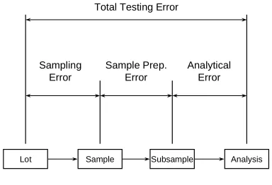
Figure 1-1 shows the relationships between the three major components of the

total variation associated with testing shelled corn for aflatoxin: sampling, sample

preparation, and analysis.

Lot Sample Subsample Analysis

Sampling Error

Sample Prep. Error

Analytical Error Total Testing Error

Figure 1-1: Total Variance partitioned into sample, sample preparation, and analytical components.

A statistical model of the aflatoxin test result, Co, can be represented by:

Equation 1-4

o

C= + +µ S SS +A

whereµ= the true aflatoxin concentration in the lot being tested, S = random deviations

of sample concentrations about the true lot concentration with expected value equal to

zero and variance σ_{C s}2_o_{( )}

(24)

comminuted sample concentration with expected value equal to zero and variance σ_{C ss}_o2₍ ₎,

and A = random deviations of analytical assay results about subsample concentration with

the expected value zero and variance σ_{C a}2_o_{( )}. If independence among the random

deviations in Equation 1-4 is assumed, the model for variance can be obtained:

Equation 1-5

σC to( ) σC so( ) σC sso( ) σC ao( )

2 = 2 + 2 + 2

where σ_{C t}2_o_{( )}

is the total variance associated with the aflatoxin test statistic Co. Total variance σ_{C t}_o2_{( )}

is the estimate of the variance among samples within the

same lot of shelled corn, which is specific to mill type, subsample size, number of

aliquots, and analytical procedure.

Variance components, σ_{C s}2_o_{( )}

and σ_{C ss}2_o₍ ₎

cannot be measured directly because of the

nested design. However, σ_{C t}_o2_{( )}, σ_{C ssa}2_o₍ ₎, and σ_{C a}2_o_{( )} can be measured directly where σ_{C ssa}_o2₍ ₎

is the combination of sample preparation and analytical variances as shown in Equation

1-6.

Equation 1-6

σC ssao( ) σC sso( ) σC ao( )

2 = 2 + 2

Then sampling and sample preparation variances can be calculated by subtraction.

Equation 1-7

σC so( ) σC to( ) σC ssao( ) 2 = 2 − 2

(25)

σC sso( ) σC ssao( ) σC ao( )

2 = 2 − 2

The sampling variance, σ_{C s}_o2_{( )}, is an estimate of the variability among replicate test

samples within each lot of shelled corn. Sample preparation variance σ_{C ss}2_o₍ ₎

is defined by

the variability among replicate subsamples obtained from the same sample comminuted

in a suitable mill.

Methods

The first experimental design (see Appendix 1) was an unbalanced nested

procedure designed to produce estimates of σ_{C t}_o2_{( )}, σ_{C ssa}2_o₍ ₎, and σ_{C s}2_o_{( )}. The notation s_C2_o is

denoted as an estimate of σ_C_o2. A bulk sample weighing approximately 45.4 kg (100 lb)

was divided into 32 test samples of 1.13 kg (2.5 lb). Each sample was comminuted in a

Romer Mill. Using 50 g subsamples, aflatoxin was extracted with methanol-water (75 +

25, v/v) in a 2:1 ratio. To purify the extract (0.5 ml), it was passed through a Mycosep

#224 column (8). The aflatoxins were derivatized using a bromide post-column

derivatization process and quantified using HPLC (9).

Two 50 g subsamples were removed from 16 of the 32 samples and one 50 g

subsample was removed from the remaining 16 samples. All subsamples were analyzed

with a single aliquot per subsample. The unbalanced design was used to keep costs

minimal while still providing enough degrees of freedom for adequate variance

estimation.

A second experiment was designed to obtain estimates of σ_{C a}2_o_{( )}. Ten subsamples

(26)

σC ao( ) 2

is the estimate of the variance among 15 replicate aliquots of extract taken from the

blender after the extraction process from a single subsample. All aliquot testing was

conducted in the same laboratory to produce an analytical variance that reflects within

laboratory variance. The results are recorded in total parts per billion (ppb) and contain

the sum of aflatoxins B1, B2, G1, and G2.

From the unbalanced nested design, the estimated variance components and the

lot aflatoxin concentration associated with each component were determined for each of

the 18 lots using the Nested procedure in SAS (10).

RESULTS AND DISCUSSION

Aflatoxin test results for all 18 lots and 32 samples can be seen in Appendix 2

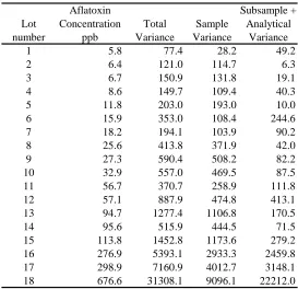
Tables 1-4. Variance estimates were obtained for eighteen lots. Table 1-1 reports

aflatoxin concentration, total variance s_{C t}2_o_{( )}, sampling variance s_{C s}2_o_{( )}, and combined

sample preparation and analytical variance s_{C ssa}2_o₍ ₎ values associated with each

contaminated lot of shelled corn. Appendix 3 shows the SAS (10) program used to

estimate the variance components. The 18 lots are ranked by aflatoxin concentration,

which ranged from about 6 to 677 ppb. In general, as the aflatoxin concentration

increases, each variance estimate increases. This reflects the results of similar variance

(27)

Table 1-1: Average aflatoxin concentration, sample variance, and combined subsampling and analytical variance

components for all 18 lots of shelled corn. **

Aflatoxin Subsample +

Lot Concentration Total Sample Analytical

number ppb Variance Variance Variance

1 5.8 77.4 28.2 49.2

2 6.4 121.0 114.7 6.3

3 6.7 150.9 131.8 19.1

4 8.6 149.7 109.4 40.3

5 11.8 203.0 193.0 10.0

6 15.9 353.0 108.4 244.6

7 18.2 194.1 103.9 90.2

8 25.6 413.8 371.9 42.0

9 27.3 590.4 508.2 82.2

10 32.9 557.0 469.5 87.5

11 56.7 370.7 258.9 111.8

12 57.1 887.9 474.8 413.1

13 94.7 1277.4 1106.8 170.5

14 95.6 515.9 444.5 71.5

15 113.8 1452.8 1173.6 279.2

16 276.9 5393.1 2933.3 2459.8

17 298.9 7160.9 4012.7 3148.1

18 676.6 31308.1 9096.1 22212.0

**Testing Plan=1.13kg sample, Romer Mill, 50 g subsample, and 1 aliquot quantified by HPLC.

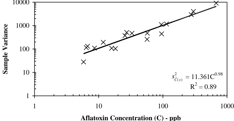
Sampling Variance

The sampling variance estimates from Table 1-1 show a linear relationship with

the mean aflatoxin concentration when plotted in full log scale (Figure 1-2). Therefore,

sampling variance was modeled by the following mathematical expression.

Equation 1-9

o( ) o C s

b

s2 =aC

where s_{C s}2_o_{( )} is the sample variance component,a and b are constants determined by

(28)

Using regression analysis, a relationship between sampling variance and aflatoxin

concentration was developed.

Equation 1-10

s_{C s}2_o_{( )} =11361. Co0 98.

with a coefficient of determination of 0.89 in the full log scale.

= 11.361C0.98 R2= 0.89 1

10 100 1000 10000

1 10 100 1000

Aflatoxin Concentration (C) - ppb

S

a

mp

le

Vari

an

ce

s

C so( ) 2

Figure 1-2: Sampling variance versus aflatoxin concentration for 1.13 kg test samples of shelled corn.

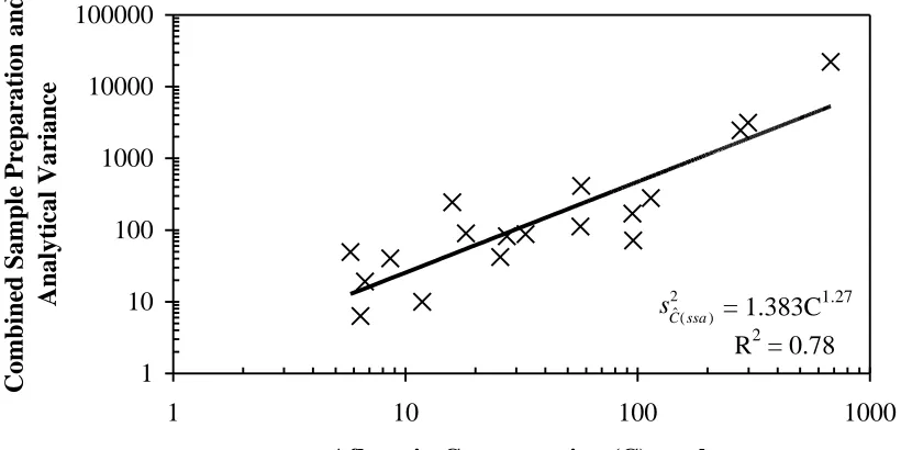
Combined Sample Preparation and Analytical Variance

Table 1-1 reports the combined sample preparation and analytical variance

estimatess_{C ssa}2_o₍ ₎

. Figure 1-3 shows the combined sample preparation and analytical

variance estimates versus aflatoxin concentration plotted in full log scale. Generally,

combined sample preparation and analytical variance estimates increased with an

(29)

was developed between the combined sample preparation and analytical variance and

aflatoxin concentration.

Equation 1-11

s_{C ssa}2_o₍ ₎ =1383. Co1 27.

= 1.383C1.27 R2= 0.78 1

10 100 1000 10000 100000

1 10 100 1000

Combine

d

Sample

Pr

ep

ar

ation

a

nd

Analytical

Variance

s

C ssao( ) 2

Figure 1-3: Combined sample preparation and analytical variance versus aflatoxin concentration for test subsamples of shelled corn using 50 g subsamples comminuted in the Romer mill, 1 aliquot per subsample, and HPLC.

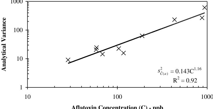
Analytical Variance

Table 1-2 shows analytical variance estimates s_{C a}2_o_{( )} among the 15 replicated test

results for each of the 10 subsamples analyzed. Generally, as the aflatoxin concentration

(30)

between the analytical variance and the aflatoxin concentration when plotted in the full

log scale. Using regression analysis, the following mathematical expression provided a

suitable relationship between the analytical variance and aflatoxin concentration.

Equation 1-12

s C

C ao( )

.

. o

2 1 16

0143

=

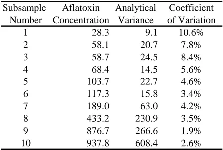
Table 1-2: Average aflatoxin concentration, analytical variance, and coefficient of variation among replicate aflatoxin test results on 15 aliquots quantified by HPLC.**

Subsample Aflatoxin Analytical Coefficient Number Concentration Variance of Variation

1 28.3 9.1 10.6%

2 58.1 20.7 7.8%

3 58.7 24.5 8.4%

4 68.4 14.5 5.6%

5 103.7 22.7 4.6%

6 117.3 15.8 3.4%

7 189.0 63.0 4.2%

8 433.2 230.9 3.5%

9 876.7 266.6 1.9%

10 937.8 608.4 2.6%

(31)

= 0.143C1.16 R2= 0.92 1

10 100 1000

Analytical

Variance

s

C ao( ) 2

Figure 1-4: Analytical variance versus aflatoxin concentration for test subsamples of shelled corn using 15 aliquots per subsample and HPLC.

Sample Preparation Variance

Once relationships are developed for s

C ssao( ) 2

and s

C ao( ) 2

, Equation 1-8 can be used to

determine sample preparation variance s

C sso( ) 2

. An equation to estimate sample

preparation variance can be calculated by subtraction of Equation 12 from Equation

1-11.

Equation 1-13

s C C

C sso( )

. .

. o . o

2 1 27 1 16

1383 0143

= −

Equation 1-13 can be simplified by regressing the difference, s

C sso( ) 2

, on aflatoxin

concentration Co. A suitable expression is shown in Equation 1-14.

(32)

s C C sso( )

.

. o

2 1 27

1254

=

Application of Results

Equations 1-10 through 1-14 estimate variances associated with testing a lot of

shelled corn for aflatoxin using a 1.13 kg sample, Romer Mill, 50 g subsample, and

HPLC. Reducing one or more of the three variance components, sampling, sample

preparation, or analytical, will reduce the total variance associated with a testing

procedure. Statistical theory indicates that an increase in quantity of material tested will

decrease variance associated with that step of the testing procedure. For example,

increasing sample size or number of sample units can reduce sampling variance;

increasing subsample size or number of subsample units can reduce sample preparation

variance; and increasing the size of the aliquot or number of aliquots taken from the

blender after the extraction process to be quantified by HPLC can reduce analytical

variance.

Equation 1-10 can be modified to predict the sampling variance for a given

sample size.

Equation 1-15

s

ns C

C so( )

. .

. o

2 113 0 98

11361

=   ⋅

wherens is the sample size in kg.

The sample preparation variance in Equation 1-14 can be modified to predict the

effect of any size subsample comminuted in the Romer mill.

(33)

s

nss C

C sso( )

.

. o

2 50 1 27

1 254

=   ⋅

wherenss is the subsample size in g.

A similar expression can be derived for the analytical variance described in

Equation 1-12. Modification of Equation 1-12 shows the effect of any number of

aliquots quantified by HPLC.

Equation 1-17

s

na C

C ao( )

.

. o

2 1 116

0143

=   ⋅

wherena is the number of aliquots.

Total variance can be estimated for any sample size, subsample size comminuted

in a Romer Mill and number of aliquots quantified by HPLC by summing Equations 1-15

through 1-17.

Equation 1-18

s

ns C nss C na C

C to( )

. . .

. _o . _o . _o

2 12 95 0 98 62 70 1 27 0143 1 16

= _  _+ _  _+ _  _

With Equation 1-18, the total variance associated with testing a contaminated lot

of shelled corn for aflatoxin at 20 ppb using a 1.13 kg sample, Romer Mill, 50 g

subsamples, and quantifying 1 aliquot per subsample using HPLC is 274.9 (CV=82.9%).

Sampling, sample preparation, and analytical variances are 214.0 (CV=73.1%), 56.3

(CV=37.5%), and 4.6 (CV=10.7%), respectively and account for 77.8, 20.5, and 1.7 % of

(34)

with sample preparation producing the next largest amount, and analytical with the least.

This follows the same pattern observed with other commodities (6, 11-15).

The effect of increasing sample size on reducing testing variability can be

demonstrated with Equation 1-18. Testing a contaminated lot of shelled corn for

aflatoxin at 20 ppb using a 5 kg sample, Romer Mill, 100 g subsamples, and quantifying

1 aliquot per subsample using HPLC produces a total variance value of 81.6

(CV=45.2%). Sampling, sample preparation, and analytical variances are 48.8

(CV=34.9%), 28.2 (CV=26.5%), and 4.6 (CV=10.7%), respectively and account for 59.8,

34.5, and 5.7 % of the total variation.

Assuming that aflatoxin test results from shelled corn follow the theory of

normally distributed variables, a lot with an aflatoxin concentration of 20 ppb and a total

variance of 81.6 implies that aflatoxin test results will fall in the range of 20±18 ppb, or

2-38 ppb, 95% of the time.

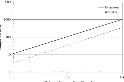
Whitaker's (7) study used similar sampling techniques, but different sample

preparation and analytical methods than this study. Only sampling variances can be

compared between the two studies. Figure 1-5 shows that Whitaker's sampling variance

is considerably less than in this study. This suggests Whitaker's assumption that his

mini-lots were representative of commercial mini-lots may be incorrect. In Figure 1-5, the slopes of

the two lines are almost parallel, which implies that Whitaker's assumption about a linear

(35)

1 10 100 1000 10000

1 10 100

S

a

mp

le

Varian

ce

Johansson Whitaker

Figure 1-5: Comparison of sampling variances for Whitaker's 1979 study to Johansson's 1998 study of variability associated with testing shelled corn for aflatoxin.

The next step would be to calculate which theoretical distribution describes the

sample distribution of shelled corn data in this study.

SUMMARY

Eighteen lots of shelled corn were tested for aflatoxin using an unbalanced nested

design. Estimates of the total variability associated with testing shelled corn for aflatoxin

were shown to increase as aflatoxin concentration increased. This also held true for each

step of the test procedure: sampling, sample preparation, and analytical variability. Using

regression analysis, mathematical expressions were developed to model all three variance

components. The expressions were used to estimate the variance for any sample size,

(36)

example, testing a lot with 20 parts per billion (ppb) aflatoxin using a 2.5 lb sample,

Romer mill and 50 g subsample, and HPLC analysis, the total, sampling, sample

preparation, and analytical variances are 274.9 (CV=82.9%), 214.0 (CV=73.1%), 56.3

(CV=37.5%), and 4.6 (CV=10.7%), respectively. The percentage of the total variance for

sampling, sample preparation, and analytical is 77.8, 20.5, and 1.7 %, respectively. As

with testing of aflatoxins in other commodities, sampling variance contributes the most

variability followed by sample preparation and then analytical variability.

REFERENCES

1. Rodricks, J. V., and Roberts, H. R. 1977. Mycotoxin Regulation in the United States. Pages 753-757 in Mycotoxins: In Human and Animal Health. Rodricks, J. V., Hesseltine, C. W., Mehlman, M. A. (eds). Illinois: Pathotox.

2. Diener, U. L., R. E. Pettit, and R. J. Cole. 1982. Chapter 13: Aflatoxins and Other Mycotoxins in Peanuts in Peanut Science and Technology. H. E. Pattee, and C. T. Young (eds). Yoakum, Texas: American Peanut Research and Education Society, Inc.

3. Anonymous. 1997. Worldwide regulations for mycotoxins 1995. FAO Food and

Nutrition Paper 64. FAO Viale della Terme di Caracalla. 00100 Rome, Italy.

4. Marshall, J. W. 1992. U. S. Department of Agriculture Federal Grain Inspection Service Aflatoxin Handbook. Sec. 4.2-4.8.

5. Cucullu, A. F., L. S. Lee, R. Y. Mayne, and L. A. Goldblatt. 1966. Determination of

aflatoxins in individual peanuts and peanut sections. Journal of American Oil

Chemists' Society 43(2):89-92.

6. Whitaker, T. B., F. E. Dowell, W. M. Hagler, Jr., F. G. Giesbrecht, and J. Wu. 1994. Variability Associated with Sampling, Sample Preparation, and Chemical Testing for

Aflatoxin in Farmer’s Stock Peanuts. Journal of AOAC International. 77:107-116.

7. Whitaker, T. B., J. W. Dickens, and R. J. Monroe. 1979. Variability Associated with

Testing Corn for Aflatoxin. Journal of the American Oil Chemists’ Society.

56:789-794.

(37)

aflatoxins B1, B2, G1, and G2 in corn, almonds, Brazil nuts, peanuts, and pistachio

nuts. Journal of AOAC International. 77:1512-1521.

9. Traag, W. A., J. M. P. Van Trijp, L. G. M. Th. Tuinstra, and W. Th. Kok. 1987. Sample clean-up and post-column derivatization for the determination of aflatoxin B1

in feedstuffs by liquid chromatography. J. Chromatogr. 396:389-394.

10. Statistical Analysis System Institute, Inc. 1996. SAS Program 6.12. Cary, NC 27513.

11. Whitaker, T. B., W. Horwitz, R. Albert, and S. Nesheim. 1996. Variability Associated with Analytical Methods Used to Measure Aflatoxin in Agricultural

Commodities. Journal of AOAC International. 79:476-485.

12. Cambell, A. D., T. B. Whitaker, A. E. Pohland, J. W. Dickens, and D. L. Park. 1986. Sampling, sample preparation, and sampling plans for foodstuffs for mycotoxin

analysis. Pure and Appl. Chem. Vol. 58, pp. 305-314.

13. Whitaker, T. B., M. E. Whiten, and R. J. Monroe. 1976. Variability Associated with

Testing Cottonseed for Aflatoxin. Journal of the American Oil Chemists’ Society.

Vol. 53, No. 7, pp. 502-505.

14. Whitaker, T. B., J. W. Dorner, F. E. Dowell, and F. G. Giesbrecht. 1992. Variability Associated with Chemical Testing Screened Farmer’s Stock Peanuts for Aflatoxin.

Peanut Science. 19:88-91.

15. Whitaker, T. B., J. W. Dickens, and R. J. Monroe. 1974. Variability of Aflatoxin

(38)

CHAPTER 2. DETERMINATION OF A SUITABLE

STATISTICAL MODEL TO SIMULATE OBSERVED

DISTRIBUTIONS OF AFLATOXIN TEST RESULTS IN

SHELLED CORN

ABSTRACT

Suitability of several theoretical distributions to predict the observed distribution

of aflatoxin test results in shelled corn is investigated in this study. Fifteen positively

skewed distributions were each fitted to 18 empirical distributions of aflatoxin test results

for shelled corn. The compound gamma distribution was selected to model the sample

aflatoxin test results for shelled corn. The method of moments technique was chosen to

estimate the parameters of the compound gamma distribution. Mathematical expressions

were developed to calculate the parameters of the compound gamma distribution for any

lot aflatoxin concentration and test procedure. Observed acceptance probabilities were

compared to operating characteristic curves predicted from the compound gamma

distribution and all 18 observed acceptance probabilities were found to lie within a 95%

confidence band.

The parameters of compound gamma were used to calculate the fraction of

aflatoxin-contaminated kernels in a lot at 20 ppb, which was estimated to be about six in

10,000.

INTRODUCTION

Regulatory guidelines that define the maximum concentration of aflatoxin

(39)

parts per billion (ppb) for foods destined for human consumption. To ensure that

consumer-ready products meet FDA aflatoxin guidelines, commodity industries and

manufacturers use aflatoxin-sampling plans or sample acceptance schemes to either

accept or reject a bulk lot based on the lot’s estimated aflatoxin concentration. A

sampling plan is defined as an aflatoxin test procedure combined with a sample

acceptance limit. The test procedure consists of sampling, sample preparation, and the

analytical steps. The sample acceptance limit is a threshold concentration that may or

may not be equal to the regulatory guideline. If the sample test result is less than or equal

to the sample acceptance limit, the bulk lot is accepted; otherwise, it is rejected.

Risks

Ideally, a lot with aflatoxin concentration,C, greater than a defined guideline, Cg,

should be rejected from entering the food chain, and a lot withC less than or equal to Cg

should be accepted. In reality, the lot aflatoxin concentrationC is estimated by

quantifying the aflatoxin C in a sample taken from the lot. The values ofo C for ao

specified lot will differ fromC because of random variation associated with sampling

(only a sample of kernels is tested), sample preparation and the analytical procedure

(2-7). The discrepancy betweenC and C lead to some lots being misclassified.o

Normally lots of shelled corn are inspected with an aflatoxin-sampling plan and

are classified either as unacceptable when the sample test result, C is greater than theo

sample acceptance limitCa, or acceptable when C is less than or equal to the sampleo

(40)

In a sampling plan, two types of misclassification can occur. The first type of

misclassification, a false positive, occurs when C > Co aand the lot is rejected when in

reality,C≤Cgor the lot is acceptable. This is also called the seller’s risk because a good

lot would be diverted from the food chain at an expense to the seller. The second type of

misclassification, a false negative occurs when Co ≤Caand the lot is accepted when in

realityC > Cgthat is, the lot is not acceptable. This misclassification is known as a

buyer’s risk because a bad lot may require additional cleaning and processing to lower

the lot aflatoxin concentration level. Also, if the unacceptable lot goes undetected, the lot

enters the food chain and becomes a potential health risk to the consumer. The frequency

of these two misclassifications occurring depends uponCg,Ca, and the design of the

sampling plan. The degree to which these two misclassifications will occur can be

evaluated with the help of an operating characteristic curve.

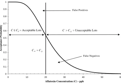
Operating Characteristic Curve

LetP{C} be the probability that a lot of shelled corn with an aflatoxin

concentrationC will be accepted by a specified sampling plan. Clearly, any reasonable

sampling plan will give a large probability of accepting a lot with a smallC and a small

(hopefully zero) probability of accepting a lot with a largeC. An operating characteristic

(OC) curve is simply a plot ofP{C} versus C. Figure 2-1 shows a typical OC curve. An

OC curve is uniquely defined by a specific testing plan and sample acceptance limit (6,

(41)

0 0.1 0.2 0.3 0.4 0.5 0.6 0.7 0.8 0.9 1

0 10 20 30 40 50 60

Accepta

nce

P

ro

ba

bility

False Positives

False Negatives

C > Cg = Unacceptable Lots

C≤Cg= Acceptable Lots

Ca = Cg

Figure 2-1: Typical operating characteristic curve showing the performance of an aflatoxin sampling plan when testing lots with aflatoxin concentration C.

Knowing the percentage of lots with a given lot concentrationC that will be

accepted and rejected by the specified sampling plan gives an indication of the

misclassification errors associated with the sampling plan. The ability to evaluate the

performance of an aflatoxin-sampling plan will provide a method to estimate the costs

involved with different sampling plans and help identify the most efficient plan for the

resources available.

Theoretical Distribution

In order to determine an OC curve, the observed distribution of sample aflatoxin

test results must either be measured or adequately described by a theoretical distribution.

(42)

distribution should be able to (1) accurately describe the observed distribution of

aflatoxin test results for a specific test procedure over a wide range of aflatoxin

concentrations, (2) contain parameters that are easily computed from experimental data

and (3) be able to be applied to practical situations.

The distribution of sample aflatoxin test results for different commodities has

been studied by several different scientists (3, 8, 15-29). Shelled corn, cottonseed, and

pistachio nuts have been investigated, but the majority of studies have been on peanuts.

These studies have shown similar characteristics about the observed distribution

of sample aflatoxin test results for the above commodities: (a) aflatoxin sample test

results taken from contaminated lots were positively skewed (>50% of sample test results

were below the lot concentration); (b) for a given lot concentration, the range between

minimum and maximum sample test results is large which indicates a large variance

associated with the test procedure; (c) the range between minimum and maximum

increases as aflatoxin concentration increases which suggests that the variance associated

with sample test results increases with aflatoxin concentration; and (d) as aflatoxin

concentration increases, the distribution of sample test results becomes less skewed and

more like the normal distribution (6).

The following distributions have been investigated as possible models of observed

distributions of sample aflatoxin test results: negative binomial (6, 15, 21, 22), compound

gamma (21-23), log normal (23, 24), truncated normal (23), Waibel (25), and

three-parameter Weibull (26-28).

(43)

suitability of several theoretical distributions to accurately predict observed distributions

of sample aflatoxin test results for shelled corn, (2) develop methods to estimate the

parameters of the theoretical distribution and (3) compare observed and predicted OC

curves to evaluate how accurately OC curves can be determined from theoretical models.

METHODS

Theoretical Distributions

Four distributions were evaluated: the compound gamma, negative binomial,

three-parameter log normal and truncated normal. See Appendix 4 for the probability

density functions associated with each distribution. Several cases of the compound

gamma distribution were evaluated where the shape parameterαwas unrestricted (CG),

set equal to 0.5 (CG0.5), 1 (CG1), 1.5 (CG1.5), 2 (CG2), and 2.5 (CG2.5). The

compound gamma, negative binomial, and truncated normal have parameters that relate

to a sample size term in the density function to allow the distribution to be adjusted for

different sample sizes (i.e. different test procedures). The three-parameter log normal

density function does not contain a sample size term, but was considered because of its

ability to fit positively skewed data.

Parameter Estimation Methods

Method of moments (MM) and maximum likelihood (ML) are the two parameter

estimation methods used in this study. The MM technique provides an easy and intuitive

method of estimation, but does not always lead to the best estimators of distributional

parameters. The ML method tends to produce good estimators, but these often can be

(44)

The ML method was used to estimate the parameters for all distributions. For

comparison, the method of moments was also used to estimate parameters of the

compound gamma and negative binomial distributions. SAS (31) procedures were used

to calculate estimates under both methods (See Appendix 5).

Goodness of Fit

The power divergence (PD) (32) test statistic was selected as the criterion to

evaluate the goodness of fit (GOF) of the theoretical distributions to the observed

distributions. The PD statistic was selected because this test is generally found to have

reasonable power against a broad range of alternatives (32). The test statistic is actually

very similar to the familiar chi-square goodness of fit test statistic. The fit was

considered acceptable if the test statistic failed to exceed the 95% critical value. The test

statistic was converted to a GOF probability where the lower the GOF probability, the

better the fit.

Observed Distribution

Bulk samples weighing approximately 45.4 kg (100 lb) were taken from each of 18

lots of shelled corn suspected of aflatoxin contamination. Each bulk sample was divided

in 32 test samples of 1.13 kg (2.5 lb) and comminuted in the Romer Mill. A 50 g

subsample was removed from each comminuted sample. Each subsample was analyzed

using high performance liquid chromatography (HPLC) (7). This provided 18 observed

distributions with 32 sample test results per distribution (See Appendix 6). An observed

(45)

RESULTS

Goodness of Fit

Table 2-1 shows the frequency that each theoretical distribution acceptably fit the

18 observed distributions. The three-parameter log normal and six cases of the

compound gamma distribution gave acceptable fits 100% of the time. The compound

gamma fit all 18 observed distributions using both the MM and ML parameter estimation

methods. Using the MM technique, the compound gamma distribution provided 100%

acceptable fits for CG1MM (compound gamma distribution withα= 1 using method of

moments), CG1.5MM, CG2MM, and CG2.5MM. When using the ML technique, the

compound gamma distribution produced 100% acceptable fits for the CG2ML

(compound gamma distribution withα= 2 using maximum likelihood) and CG2.5ML.

(46)

Table 2-1: The number of times each theoretical distribution provided an acceptable fit to the 18 observed distributions of sample test results using the power divergence test.

Parameter Estimation Acceptable Fitc

Distributiona Methodb Number %

Three-Parameter Log Normal ML 18 100%

CG1 MM 18 100%

CG1.5 MM 18 100%

CG2 MM 18 100%

CG2.5 MM 18 100%

CG2 ML 18 100%

CG2.5 ML 18 100%

CG1 ML 17 94%

CG1.5 ML 17 94%

CG ML 17 94%

Truncated Normal ML 15 83%

CG0.5 MM 14 78%

CG0.5 ML 14 78%

Negative Binomial ML 10 56%

Negative Binomial MM 6 33%

a

CG = compound-gamma;

CG0.5 = special case of the compound-gamma where shape parameter = 0.5; CG1 = special case of the compound-gamma where shape parameter = 1; CG1.5 = special case of the compound-gamma where shape parameter = 1.5; CG2 = special case of the compound-gamma where shape parameter = 2; CG2.5 = special case of the compound-gamma where shape parameter = 2.5;

b

ML = maximum likelihood MM = method of momemnts

c

Acceptable Fit = null hypothesis not rejected at the 5% confidence level.

The negative binomial distribution has a problem predicting the percent zero

aflatoxin sample values when a lot contains a high percentage of zero sample values. The

negative binomial distribution does however model the positive aflatoxin test results

adequately. The compound gamma and the three-parameter log normal distributions

were able to model the positively skewed distributions with high percent zero aflatoxin

sample values.

The three-parameter log normal cannot be statistically modified to predict the

(47)

parameters change as the sample size is varied. Statistically incorporating a sample size

term into the log normal distribution was investigated, but no acceptable results were

found. The remaining theoretical distributions investigated in this study can be modified

to predict the distribution of sample test results for sample sizes other than that used in

this study (15, 23).

In Table 2-1, four out of the six compound gamma distributions that acceptably fit

all 18 observed distributions were fitted using the MM as the parameter estimation

technique. Only these four theoretical distributions were considered since the MM

provides GOF results equivalent to the ML technique and has simpler computational

formulas to adjust for changes in testing procedure.

The four compound gamma distributions (CG1MM, CG1.5MM, CG2MM and

CG2.5MM) where parameters were estimated using the MM technique were evaluated to

determine which of these four distributions had the most best fits. A best fit is defined as

the theoretical distribution that fit an observed distribution with the lowest GOF

probability. Table 2-2 shows the percentage of best fits each of the theoretical

distributions produced. The CG2.5MM tied with CG2MM with the highest number of

(48)

Table 2-2: Number of times each theoretical distribution provided a best fit to the 18 observed distributions of sample test results when using the power divergence test.

Parameter Estimation Best Fitc

Distributiona Methodb Numberd %

CG2.5 MM 10 56%

CG2 MM 10 56%

CG1.5 MM 8 44%

CG1 MM 7 39%

a

CG1 = special case of the compound-gamma where shape parameter = 1; CG1.5 = special case of the compound-gamma where shape parameter = 1.5; CG2 = special case of the compound-gamma where shape parameter = 2; CG2.5 = special case of the compound-gamma where shape parameter = 2.5;

b

MM = method of momemnts

c

Best Fit = theoretical distribution with lowest GOF probability.

d

Sum of Number of Best Fits > 18 due to ties

Table 2-3 shows the average GOF probability for each distribution. Averaging

the GOF probability compares how well a theoretical distribution fit all observed

distributions as a group. A better fit would entail a lower average GOF probability. The

CG2.5MM produced the lowest average GOF probability followed by CG2MM,

CG1.5MM and CG1MM respectively.

Table 2-3: Average of all 18 power divergence test results for each theoretical distribution.

Parameter Estimation Average

Distributiona Methodb GOF Testsc

CG2.5 MM 0.51

CG2 MM 0.52

CG1.5 MM 0.57

CG1 MM 0.63

a

CG1 = special case of the compound-gamma where shape parameter = 1; CG1.5 = special case of the compound-gamma where shape parameter = 1.5; CG2 = special case of the compound-gamma where shape parameter = 2; CG2.5 = special case of the compound-gamma where shape parameter = 2.5;

b

c

Average of GOF test = average of the GOF probabilities for all 18 distributional fits.

(49)

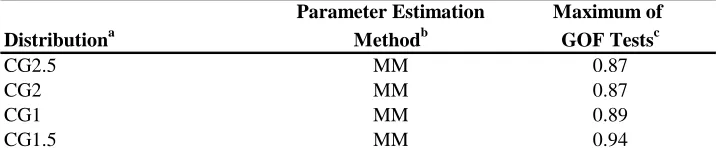
a theoretical distribution is. The CG2.5MM and CG2MM tied with the lowest maximum

GOF probability value of 0.87.

Table 2-4: Maximum value of the power divergence test for each theoretical distribution.

Parameter Estimation Maximum of

Distributiona Methodb GOF Testsc

CG2.5 MM 0.87

CG2 MM 0.87

CG1 MM 0.89

CG1.5 MM 0.94

a

CG = compound-gamma;

CG0.5 = special case of the compound-gamma where shape parameter = 0.5; CG1 = special case of the compound-gamma where shape parameter = 1; CG1.5 = special case of the compound-gamma where shape parameter = 1.5; CG2 = special case of the compound-gamma where shape parameter = 2; CG2.5 = special case of the compound-gamma where shape parameter = 2.5;

b

c

Maximum of GOF Tests = maximum GOF probability that a theoretical distribution produced.

Table 2-5 summarizes results of Tables 2-1 through 2-4 to help determine which

of the four theoretical distributions would best model sample test results of shelled corn

for aflatoxin. Each theoretical distribution acceptably fit all 18 observed distributions.

The percentage of best fits is tied between CG2.5MM and CG2MM with 56% each. The

CG2.5MM distribution has the lowest average GOF probability (0.51) while CG2.5MM

(50)

Table 2-5: Summary comparison for each of the theoretical distributions. Percentage of acceptable fits, percentage of best fits, average of GOF tests, and maximum values of GOF tests are included.

CG2.5MMa CG2MMb CG1.5MMc CG1MMd

Acceptable Fitse 100% 100% 100% 100%

Best Fitsf 56% 56% 44% 39%

Average of GOF testsg 0.51 0.52 0.57 0.63

Maximum of GOF testh 0.87 0.87 0.89 0.94

a

CG2.5MM = special case of the compound-gamma where shape parameter = 2.5 and method of moments is the parameter estimation technique.

b

CG2MM = special case of the compound-gamma where shape parameter = 2 and method of moments is the parameter estimation technique.

c

CG1.5MM = special case of the compound-gamma where shape parameter = 1.5 and method of moments is the parameter estimation technique.

d

CG1MM = special case of the compound-gamma where shape parameter = 1 and method of moments is the parameter estimation technique.

e

Acceptable Fit = null hypothesis not rejected at the 5% confidence level.

f

Best Fit = theoretical distribution with GOF acceptance probability.

g

Average of GOF tests = sum of the GOF probabilities for all 18 distributional fits.

h

Maximum of GOF Tests = maximum GOF probability that a theoretical distribution produced. Distribution

The CG2.5MM was chosen to model the observed distribution of aflatoxin sample

test results for shelled corn. Table 2-6 shows for each lot, the three compound gamma

distribution parameters determined by the method of moments and GOF probability

results as determined by the power-divergence test. Figure 2-2 shows an example of the

CG2.5MM theoretical distribution compared to the observed distribution for lot 10. Very

little difference between the two distributions can be noted (See Table 2-6, lot 10, PD test

Develop Methods To Evaluate the Performance of Aflatoxin Sampling Plans for Shelled Corn.

ABSTRACT

DEVELOP METHODS TO EVALUATE THE PERFORMANCE OF

AFLATOXIN SAMPLING PLANS FOR SHELLED CORN

ANDERS STURE JOHANSSON

BIOLOGICAL AND AGRICULTURAL ENGINEERING

APPROVED BY:

DEDICATION

I would like to dedicate this dissertation

to my father

Anders Daniel Johansson

who in our short time together provided me with a lifetime of morals

and values,

to my grandmother

Mammaw

who was always there to support me (many times financially)

through all of life's challenges,

to my parents

Teak and Betsey Edgeworth

BIOGRAPHY

ACKNOWLEGDEMENTS

TABLE OF CONTENTS

LIST OF TABLES

LIST OF FIGURES

GENERAL INTRODUCTION

References

CHAPTER 1.

ESTIMATION OF VARIANCE COMPONENTS

ASSOCIATED WITH TESTING SHELLED CORN FOR

AFLATOXIN

ABSTRACT

INTRODUCTION

EXPERIMENTAL PROCEDURE

RESULTS AND DISCUSSION

SUMMARY

REFERENCES

CHAPTER 2.

DETERMINATION OF A SUITABLE

STATISTICAL MODEL TO SIMULATE OBSERVED

DISTRIBUTIONS OF AFLATOXIN TEST RESULTS IN

SHELLED CORN

ABSTRACT

INTRODUCTION

METHODS

RESULTS