Learning Embeddings for Academic Papers

(1)

Scholarship at UWindsor

Electronic Theses and Dissertations Theses, Dissertations, and Major Papers

9-6-2019

Learning Embeddings for Academic Papers

Yi Zhang

University of Windsor

Follow this and additional works at: https://scholar.uwindsor.ca/etd

Recommended Citation Recommended Citation

Zhang, Yi, "Learning Embeddings for Academic Papers" (2019). Electronic Theses and Dissertations. 7855.

https://scholar.uwindsor.ca/etd/7855

This online database contains the full-text of PhD dissertations and Masters’ theses of University of Windsor students from 1954 forward. These documents are made available for personal study and research purposes only, in accordance with the Canadian Copyright Act and the Creative Commons license—CC BY-NC-ND (Attribution, Non-Commercial, No Derivative Works). Under this license, works must always be attributed to the copyright holder (original author), cannot be used for any commercial purposes, and may not be altered. Any other use would require the permission of the copyright holder. Students may inquire about withdrawing their dissertation and/or thesis from this database. For additional inquiries, please contact the repository administrator via email

(2)

By

Yi Zhang

A Dissertation

Submitted to the Faculty of Graduate Studies through the School of Computer Science in Partial Fulfillment of the Requirements for

the Degree of Doctor of Philosophy at the University of Windsor

Windsor, Ontario, Canada

2019

c

(3)

by

Yi Zhang

APPROVED BY:

Y. Zou, External Examiner Queen’s University

J. Wu

Department of Electrical and Computer Engineering

M. Kargar

School of Computer Science

D. Wu

School of Computer Science

J. Lu, Advisor School of Computer Science

(4)

I. Co-Authorship

I hereby certify that this dissertation incorporates material that is the result of joint

re-search, as follows: My research was conducted under the supervision of my advisor Prof.

Jianguo Lu. Parts of Chapter 3 of the thesis was co-authored with Dr. Ofer Shai under

the supervision of my advisor Prof. Jianguo Lu. Chapter 3, 4, 5, and 6 were co-authored

with Fen Zhao under the supervision of my advisor Prof. Jianguo Lu. In all cases, the

key ideas, primary contributions, experimental designs, data analysis, interpretation, and

writing were performed by the author, and the contribution of co-authors was primarily

through the discussion of technical content, data pre-processing, and proofreading of the

published manuscripts.

I am aware of the University of Windsor Senate Policy on Authorship and I certify that

I have properly acknowledged the contribution of other researchers to my thesis, and have

obtained written permission from each of the co-author(s) to include the above material(s)

in my thesis.

I certify that, with the above qualification, this thesis, and the research to which it

refers, is the product of my own work.

II. Previous Publications

This dissertation includes the extended or original version of the papers that have been

previously published/submitted for publication in peer reviewed conferences and journals,

as follows:

• Yi Zhang, Jianguo Lu, Ofer Shai. 2018. Improve Network Embeddings with

Reg-ularization. In Proceedings of the 27th ACM International Conference on Informa-tion and Knowledge Management (CIKM ’18). ACM, New York, NY, USA, pp. 1643-1646. doi:10.1145/3269206.3269320 The data and code are publicly available at

http://zhang18f.myweb.cs.uwindsor.ca/n2v_r(Chapter 3).

• Yi Zhang, Fen Zhao, Jianguo Lu. 2019. ShortWalk: Long Random Walks Considered

Harmful for Network Embeddings on Directed Graphs. The 3rd Workshop of Het-erogeneous Information Network Analysis and Applications, CIKM 2019 Workshop.

Accepted. The data and code are publicly available athttp://zhang18f.myweb.cs.

(5)

are publicly available athttp://zhang18f.myweb.cs.uwindsor.ca/p2v(Chapter 3, 5 and 6).

• Fen Zhao, Yi Zhang, Jianguo Lu, Ofer Shai. 2019. Measuring academic influence

us-ing heterogeneous author-citation networks. Scientometrics, 118(3):1119–1140. ISSN 1588-2861. doi: 10.1007/s11192-019-03010-5. The data and code are publicly

avail-able athttp://zhang18f.myweb.cs.uwindsor.ca/apn (Chapter 6).

• Fen Zhao, Yi Zhang, Jianguo Lu. 2019. Author Embeddings on Heterogeneous

Networks. The 3rd Workshop of Heterogeneous Information Network Analysis and Applications, CIKM 2019 Workshop. Accepted. The data is publicly available at

http://zhang18f.myweb.cs.uwindsor.ca/a2v(Chapter 6).

I certify that I have obtained a written permission from the copyright owner(s) to include

the above published material(s) in my thesis. I certify that the above material describes

work completed during my registration as a graduate student at the University of Windsor.

III. General

I declare that, to the best of my knowledge, my thesis does not infringe upon anyone’s

copyright nor violate any proprietary rights and that any ideas, techniques, quotations,

or any other material from the work of other people included in my thesis, published or

otherwise, are fully acknowledged in accordance with the standard referencing practices.

Furthermore, to the extent that I have included copyrighted material that surpasses the

bounds of fair dealing within the meaning of the Canada Copyright Act, I certify that I

have obtained a written permission from the copyright owner(s) to include such material(s)

in my thesis. I declare that this is a true copy of my thesis, including any final revisions,

as approved by my thesis committee and the Graduate Studies office, and that this thesis

(6)

Academic papers contain both text and citation links. Representing such data is crucial

for many downstream tasks, such as classification, disambiguation, duplicates detection,

recommendation and influence prediction. The success of Skip-gram with Negative

Sam-pling model (hereafter SGNS) has inspired many algorithms to learn embeddings for words,

documents, and networks. However, there is limited research on learning the representation

of linked documents such as academic papers.

This dissertation first studies the norm convergence issue in SGNS and propose to use

an L2 regularization to fix the problem. Our experiments show that our method improves

SGNS and its variants on different types of data. We observe improvements upto 17.47% for

word embeddings, 1.85% for document embeddings, and 46.41% for network embeddings.

To learn the embeddings for academic papers, we propose several neural network based

algorithms that can learn high-quality embeddings from different types of data. The

algo-rithms we proposed are N2V (network2vector) for networks, D2V (document2vector) for

documents, and P2V (paper2vector) for academic papers. Experiments show that our

mod-els outperform traditional algorithms and the state-of-the-art neural network methods on

various datasets under different machine learning tasks.

With the high quality embeddings, we design and present four applications on real-world

datasets, i.e., academic paper and author search engines, author name disambiguation, and

(7)

I would like to express my deepest gratitude to my supervisor, Dr. Jianguo Lu, for his

valuable assistance, useful guidance, insightful comments, and considerable encouragements

to complete this thesis.

I also would like to express my appreciation to Dr. Ying Zou, Dr. Jonathan Wu, Dr.

Dan Wu, and Dr. Mehdi Kargar. Thank you all for your valuable comments and suggestions

to this thesis.

Meanwhile, I would like to thank Dr. Ofer Shai for his precious assistance, scholarly

knowledge and enthusiasm. Great deals appreciated go to the contribution of Mr. Zeeshan

Mansoor for the efforts he made on retrofitting model and Mr. Ziyang Tian for collecting

the data for experiments.

In addition, I want to send my appreciation to the school of Computer Science and

Meta Team from Chan Zuckerberg Initiative for supporting my work through my advisor’s

grants.

Last but not least, I owe special thanks to my wife, Fen Zhao, for her infinite love and

support. It is also my privilege to thank my parents, my parents-in-law, my brother and

(8)

DECLARATION OF CO-AUTHORSHIP/PREVIOUS PUBLICATION III

ABSTRACT V

ACKNOWLEDGEMENTS VI

LIST OF TABLES X

LIST OF FIGURES XII

1 Introduction 1

1.1 Introduction . . . 1

1.2 Challenges . . . 3

1.3 Contributions . . . 4

1.4 The structure of the dissertation . . . 6

2 Background and Related Works 8 2.1 Word embeddings . . . 8

2.1.1 Co-occurrence matrix . . . 9

2.1.2 Word2vec . . . 11

2.1.3 Implementation details of SGNS . . . 21

2.1.4 GloVe . . . 26

2.2 Document embeddings . . . 27

2.2.1 Traditional methods . . . 27

2.2.2 Paragraph Vector . . . 28

2.2.3 Other approaches . . . 29

2.3 Network embeddings . . . 30

2.3.1 DeepWalk . . . 31

2.3.2 Node2vec . . . 32

2.3.3 LINE . . . 33

2.4 Linked document embeddings . . . 35

2.4.1 TADW . . . 36

2.4.2 LDE . . . 37

2.4.3 Paper2vec . . . 38

2.5 Summary . . . 39

3 Network Embeddings 40 3.1 ShortW alk – Directed graph embeddings . . . 40

3.1.1 The Dilemma . . . 41

3.1.2 Our method . . . 43

3.1.3 Experiments . . . 45

3.1.4 Conclusion . . . 51

3.2 Norm convergence issue . . . 52

3.2.1 Performance degeneration over iteration . . . 53

(9)

3.3 N2V . . . 58

3.3.1 Scalability issue . . . 58

3.3.2 Our method . . . 61

3.3.3 Compare with existing methods . . . 64

3.4 Experiments . . . 65

3.4.1 Datasets . . . 65

3.4.2 Experiment setup . . . 69

3.4.3 Classification task . . . 70

3.4.4 Link prediction task . . . 75

3.4.5 Optimum number of training pairs . . . 78

3.4.6 Analysis . . . 79

3.5 L2 regularization on word and document embeddings . . . 82

3.5.1 Word embeddings . . . 82

3.5.2 Document embeddings . . . 88

3.6 Summary . . . 94

4 Document Embeddings 95 4.1 Introduction . . . 95

4.2 Related works . . . 96

4.3 Our method . . . 97

4.4.2 Results and analysis . . . 104

4.4.3 Impact of weight . . . 106

4.5 Case study . . . 107

4.6 Summary . . . 110

5 Paper Embeddings 111 5.1 Introduction . . . 111

5.2 Our method . . . 112

5.2.1 Weight of components . . . 115

5.2.2 Regularization and optimization . . . 117

5.2.3 Compare with existing works . . . 120

5.3.1 Datasets . . . 124

5.3.2 Text only . . . 125

5.3.3 Link only . . . 128

5.3.4 Linked text . . . 132

5.4 Compare with concatenation . . . 136

5.5 Impact of weight . . . 136

5.6 Paper clustering . . . 139

5.7 Analysis . . . 142

(10)

6.1.1 Introduction . . . 145

6.1.2 Heterogeneous Author Paper Network . . . 146

6.1.3 Datasets . . . 148

6.1.4 Author Embeddings . . . 149

6.1.5 Author Search Engine . . . 156

6.1.6 Conclusions . . . 156

6.2 Author name disambiguation . . . 157

6.2.3 Experiment and results . . . 160

6.3 Similar paper search engine . . . 160

6.3.2 Experiment . . . 162

6.3.3 Compare with Google Scholar and Semantic Scholar . . . 163

6.4 Paper influence prediction . . . 165

6.5 Summary . . . 167

7 Conclusions and Future Directions 168 7.1 Discussions and conclusions . . . 168

7.2 Future directions . . . 169

REFERENCES 172

(11)

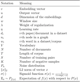
2.1 Summary of the notations. . . 9

2.2 The word-context co-occurrence matrix retrieved from Figure 2.1. Row i

denotes word wi and column j is context cj. Each entry Mi,j is the

co-occurrence between wordwi and contextcj, which is the count of wi and cj

appears in the same sliding window. . . 10

2.3 The word-context co-occurrence for w5 retrieved from Figure 2.2. . . 12

3.1 Top visited webpages in WebGoogle. Webpages are sorted by their

occur-rence in DeepWalk100_{. . . .} ₄₁

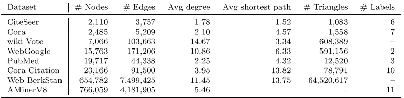
3.2 Statistics of datasets. We also list average shortest paths and number of

tri-angles for smaller graphs to understand their structure. The average shortest

path and number of triangles are not reported for AMinerV8 due to its large

size. . . 47

3.3 Performance of classification task. Scores are averaged from 5 models. Each

model produce one micro F1 score by 10-fold cross validation. . . 48

3.4 AUC score of link prediction. 10-fold cross-validation. 5 embeddings per

dataset per method. . . 50

3.5 Statistics of 33 networks. . . 69

3.6 Micro-F1 on classification task, training ratio is 8% for Flickr and YouTube

and 80% for the resets. . . 71

3.7 Macro-F1 on classification task, training ratio is 8% for Flickr and YouTube

and 80% for the resets. . . 71

3.8 Statistics of 4 Groups in different datasets. . . 74

3.9 Statistics of the corpora for word embeddings. |Voc|is the vocabulary size. 82

3.10 Summary of similarity test cases. . . 83

3.11 Comparison of W2V and W2VR on Text8, News2010 and Wikipedia. The

performance is obtained when the iteration is 50 for Text8, 10 for News2010,

and 2 for Wikipedia. Each data cell is an average of five independent runs. 85

(12)

tion task. . . 92

4.1 Best weight hyper-parameters for D2V. . . 104

4.2 F1 scores in the document classification task. . . 104

5.1 The number of training samples per iteration. Window size is 5. . . 115

5.2 Statistics of datasets. . . 125

5.3 Best parameters for D2V. . . 126

5.4 Micro-F1 of paper classification – Text only task. LDA and LSA do not scale to MAG dataset so we can not report the performance. . . 126

5.5 Best parameters for N2V. . . 130

5.6 Micro-F1 of paper classification – Link only task. . . 130

5.7 Best parameters for P2V, pis walk probability. . . 133

5.8 Micro-F1 of paper classification – Linked text task. . . 133

5.9 Information of the highlighted papers in Figure 5.14. . . 136

5.10 Statistics of the labels in the paper clustering task. . . 140

5.11 Best parameters for P2V in clustering task,pis walk probability. . . 142

6.1 Statistics of AMiner and Health datasets. . . 149

6.2 Statistics of ACM fellows, Turing Award Winners, and Nobel Prize Winners. 149 6.3 Average F1 scores of binary classification for ACM Fellows on different net-works. . . 151

6.4 F1 scores of author name disambiguation. It also shows the improvement of P2V against LDE. . . 159

6.5 Comparison with Google Scholar and Semantic Scholar. . . 163

6.6 Top 5 similar papers to Support Vector Networks in AMinerV10. The high-lighted paper is irrelevant to SVM. Citation count is retrieved via Google Scholar on Sept 2018. . . 164

(13)

1.1 A screenshot of an academic paper. The first page in Panel (a) has multiple

entities marked in different colors. Here authors are yellow, institutions are

blue, keywords are red, venue is purple and publication year is green. This

paper also links to other related papers via citation links as illustrated in

Panel (b). . . 2

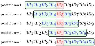
2.1 An example of a basic sliding window when capturing word-context

co-occurrence information. The corpus is a set of words in a specific order.

Suppose window size C = 5, the window moves from left to right and

cap-tures 5 words at each time. Every two words appeare in that window count

as one co-occurrence. We can record the co-occurrence count in a matrix

listed in Table 2.2. . . 10

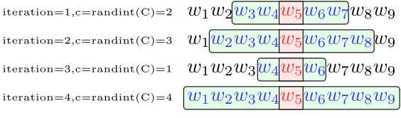
2.2 An example of skip-gram window in word2vec. The corpus is a set of words in

a specific order. LetC = 4 be the window size,w5be the center word, which is

the target word we want to learn the embedding for in this example. Function

randint(C) returns a random integer in a range of (0, C). In each iteration,

we generate a window size c = randint(C) and collect the (word,context)

pairs within the window. For example, in the third iteration, cis 1, we take

1 neighbor left and right to the center word w5. The (word,context) pairs

generated in this step is (w5, c4),(w5, c6). . . 12

2.3 CBOW as Neural Network with one hidden layer. . . 13

2.4 Comparison between Softmax and Hierarchical Softmax. Panel (a) illustrates

the multi-class classification using Softmax. Panel (b) shows the Hierarchical

Softmax. It solves the multi-class classification problem via multiple binary

classifiers where labels are the binary code of the target on the Huffman tree.

In this example,w5 is the target word and the corresponding binary code on

the Huffman tree is (1,0,0). . . 14

(14)

the multi-class classification using Softmax. Panel (b) shows the Negative

Sampling in which the negative samples are retrieved randomly via noise

distribution. . . 16

2.7 Preprocessing Subsampling of the raw text. . . 23

2.8 An example of preprocessing. The sentence is retrieved from Text8 dataset. 25

2.9 A snapshot of embeddings in Text8 during the training. Panel (a) is the

snapshot after initialization. We can see that words randomly assigned in

the vector space. Panel (b) is the snapshot token after 5_×104 samples been

trained. “zero” has been pushed to the left and “british” is moving to the

right towards “american”. Panel(c) is the snapshot after 105 samples been

trained. Words are separated into two groups by their semantic meanings. 26

2.10 Random walk in DeepWalk. . . 31

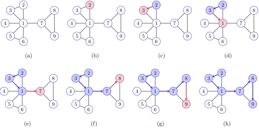
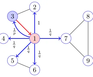
2.11 An example of biased random walk probability in node2vec. . . 32

2.12 An example of academic papers. . . 35

2.13 The structure of TADW. Mis the DeepWalk co-occurrence matrix. WT _is

embedding matrix, T is the text information matrix. Hconnects W and T. 36

3.1 Distribution of occurrence by differentl in DeepWalk. . . 42

3.2 Comparison of SGNS and pair-wise combination. The Pearson’s Correlation

Coefficient between them is 1₋2_×10−6_{. . . .} ₄₅

3.3 Performance of classification task. Each model produce one micro F1 score

by 10-fold cross validation. Panel(a) reports the F1 score averaged from 5

models. The shaded area indicate the standard deviation. Panel(b) shows

the corresponding improvement using DeepWalk as the baseline. . so the

traces should not be very different from ShortWalk. . . 48

3.4 Performance of Link Prediction task. Each model produce one AUC score

by 10-fold cross validation. Then the reported AUC score is averaged from

5 models. Panel(a) shows the AUC score of ShortWalk and DeepWalk. The

shaded area indicate the standard deviation. Panel(b) shows the

correspond-ing improvement uscorrespond-ing DeepWalk5 _{as the baseline. . . .} ₅₀

(15)

3.7 2D plot of PubMed. . . 52

3.8 Performance degeneration on network embedding algorithms. . . 53

3.9 L2-norm of vectors – BlogCatalog. . . 55

3.10 Sigmoid function. The output is in range of (0,1) . . . 57

3.11 Norms of the vectors in network embeddings – L2 regularization on embed-ding vectors only. . . 58

3.12 Norms of the vectors in network embeddings – L2 regularization on embed-ding vectors and output vectors. . . 59

3.13 An example of random walk based network embedding algorithms. It uses a walker to generate the walking paths. Training pairs are captured by a skip-gram window, and are learned by SGNS. . . 59

3.14 An example of LINE. It uses random edge sampling to generate the training samples. . . 61

3.15 An example of N2V sampling. The red node represents the start node. Blue line is the visited path. Red lines represent the current walking path and the dashed line represents the random jump. . . 62

3.16 Comparison between different sampling strategies in Karate Club. Panel(a) shows the original network with ground true labels. Panel (b) to (u) show the training sample pairs generated for different target nodes by different sampling strategies. The red node indicates the training target ( the input node ). The green nodes are the corresponding neighbors. The color and size reflect the probability that a green node is selected as an output of the red node. . . 66

3.17 Pearson’s correlation coeefficiant of different sampling strategies. . . 67

3.18 Degree distribution of 33 networks. . . 68

3.19 Comparison between walking probability in N2V and window size in DeepWalk. 70 3.20 Micro-F1 and Macro-F1 of node classification task. First row shows the performance, Second row is the improvement. . . 72

(16)

the improvement for small nodes and Panel (b) is for large nodes. . . 75

3.23 AUC of Link prediction task – Hadamard operator. . . 77

3.24 AUC of Link prediction task – average operator. . . 78

3.25 Optimum training examples for different datasets. . . 79

3.26 Visualization on Cora. Red dots represent papers inGenetic Algorithms. . . 80

3.27 Visualization on PubMed. . . 81

3.28 Word frequency distribution of Text8, News2010, and Wikipedia. . . 82

3.29 An example of analogy test. The figures use the relation of ‘Beijing’ is the capital of ‘China’ to infer the capital for ‘Japan’. . . 85

3.30 Comparison of W2V and W2VR on similarity and analogy task. Training data is Text8. . . 86

3.31 Comparison of W2V and W2VR. Examples are traken randomly from Google Analogy test case – Country-capital. . . 87

3.32 L2-norm of the word and context embeddings during the training on News2010 and Wikipedia. . . 88

3.33 Document length distribution and word frequency distribution of different datasets. . . 89

3.34 Comparison between PV-DBOW and PV-DBOWR on document classifica-tion task. . . 92

3.35 An example of mis-classified documents in IMDB. Left plot shows embed-dings generated by PV-DBOW and right is for PV-DBOWR. We use t-SNE to reduce 100 dimensional embeddings into 2 dimensions. . . 93

3.36 The content of IMDB document with id 40906 corresponding to Figure 3.35. This document is classified as a positive review in PV-DBOW but correctly identified by PV-DBOWR. . . 94

4.1 The structure of D2V. . . 98

(17)

smaller α is, the less weight learned from the word-word pairs. The red dot

indicates the best hyper-parameter. The green triangle is the performance

of D2V eqweighted. The blue diamond represents the D2V unweighted model.106

4.4 Document embeddings in arXiv2019. We use PCA to reduce the dimension of

document embeddings from 100 to 2. Documents are split into three groups.

Each color represents a group. . . 107

4.5 Pair-wised cosine similarity of seven documents in arXiv2019. . . 108

4.6 Word embeddings in arXiv2019. We use PCA to reduce the dimension of

words embeddings from 100 to 2. Words are split into three groups. Each

color represents a group. . . 109

4.7 Pair-wised cosine similarity of seven words in arXiv2019. . . 109

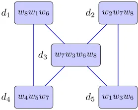
5.1 An example of three components in academic papers. Panel (a) shows

an example of academic papers. Five papers connected by citation links.

{d1, d2, ..., d5} are papers; {w1, w2, ..., w8} are corpus in the papers. Papers

contain words and connect to others by citation links. Panel (b) shows

train-ing samples retrieved from three components. . . 113

5.2 P2V as Neural Networks. Panel (a) (b) and (c) illustrate the learning

pro-cedure of sample (w3, w8), (d3, w3), and (d3, d5) respectively. The training

samples are derived from Figure 5.1. . . 116

5.3 Norm convergence issue on Cora dataset. Panel (a) shows the performance

of embeddings during the training. Panel(b) shows the mean of vectors’ L2

norms in each group. Each group contains 25 samples. 100 samples in total. 117

5.4 Norm and performance with L2 regularization on Cora. The plots are

gen-erated under the same strategy as Figure 5.3. . . 120

5.5 The structure of LDE. Panel (a) is LDE-doc and Panel (b) shows LDE-link. 121

5.6 An example of vector concatenation. . . 123

5.7 An example of retrofitting. Papers connect to each other through links. Each

paperdi is associated with its document embeddings ˆvi retrieved from D2V

and a paper embedding vi. In this example, we learn the paper embedding

(18)

the overall performance. Panel (b) compares D2V with LDE-Doc,

PV-DBOW, and PV-DM. Panel (c) illustrates the effect of weight in D2V models.127

5.9 2D plot of Cora for text-only task. The dimension of embeddings is reduced

from 100 to 2 by t-SNE. . . 129

5.10 Performance on Link only task corresponding to Table 5.6. Panel (a) shows the overall performance of each method. Panel (b) compares the N2V with random walk based methods. Panel (c) compares the performance between N2V and random edge based methods. . . 131

5.11 2D plot of network embeddings on Cora. The dimension of embeddings are reduced from 100 to 2 by t-SNE. . . 132

5.12 Performance on Linked Text task corresponding to Table 5.8. Panel (a) shows the overall performance. Panel (b) compares P2V with LDE, Retrofitting and Concatenation methods. Panel (c) illustrates the effect of weight in P2V. . 134

5.13 2D plots of paper embeddings on Cora. The dimension of embeddings are reduced from 100 to 2 by t-SNE. . . 135

5.14 An example of mis-classified papers in AminerV10. Embeddings are gener-ated by D2V, N2V, Concatenation and P2V. We use t-SNE to reduce 100 dimensional embeddings into 2 dimension. The orange dots represent pa-pers published in ICSE. Blue dots are VLDB papa-pers. Red and blue dots are papers misclassified by D2V and Concatenation. . . 137

5.15 Impact ofα,β, and γ on Cora. . . 137

5.16 Impact ofα,β, and γ on arXiv title. . . 138

5.17 Normalized Mutual Information of the paper clustering task. . . 140

5.18 Nine papers retrieved from P2V and LDE. The dimension of vectors is reduce from 100 to 2 via PCA. Nine papers are split into four groups manually according to the research topic. Each color represents a group of papers. . 143

(19)

5 papers and 8 authors. Panel(b), (c), and (d) are the corresponding APN,

ACN, and ACCN, respectively. . . 147

6.2 Performance of classification on different networks. . . 150

6.3 2D plot of ACM Fellows. . . 152

6.4 NMI of clustering for 60 Turing Award Winners. . . 153

6.5 Dendrogram and the corresponding heatmaps for 60 Turing Award Winners. 154 6.6 2D plot of Nobel Prize Winners. We use t-SNE to reduce the dimension of embeddings from 100 to 2. . . 155

6.7 A screenshot of Similar Author Search Engine . . . 156

6.8 F1 scores of author name disambiguation. . . 159

6.9 A screenshot of Similarity Search Engine. It shows the most similar papers to [Mikolov et al., 2013b] retrieved by P2V. The paper introduces “word2vec” algorithm . User can also search similar papers by D2V and N2V for com-parison. . . 161

6.10 The precision atk on GIST dataset. . . 162

6.11 Comparison with Google Scholar and Semantic Scholar. . . 163

6.12 Paper influence prediction workflow. Blue data represents the snapshot of 2015, green data represents the snapshot of 2016, and red is the snapshot of 2017. . . 165

(20)

Introduction

Academic papers contain rich information and attract increasing attention from industry

and academia. The size of academic papers is large in real-world, making it challenging to

study and analyze. In the past few years, embeddings techniques become a popular method

to represent different types of data such as words [Mikolov et al., 2013b, Pennington et al.,

2014], documents [Le and Mikolov, 2014] and networks [Perozzi et al., 2014, Tang et al.,

2015b, Grover and Leskovec, 2016]. It has been proven effective for many downstream tasks

such as classification [Zhou et al., 2016], clustering [Viegas et al., 2019] etc. This dissertation

focuses on how to learn high quality embeddings from academic papers. This chapter first

gives an overview of the research topic in this dissertation. It outlines the main challenges in

learning embeddings for academic papers. Then, the main contributions of this dissertation

are summarized and the structure of the remaining chapters will be introduced.

1.1 Introduction

Scientific publications, especially academic papers, have become crucial resources in both

academia and industry. In addition to text content, academic papers also link to each

other via citation links. Meanwhile, there are other entities in a paper, such as keyword(s),

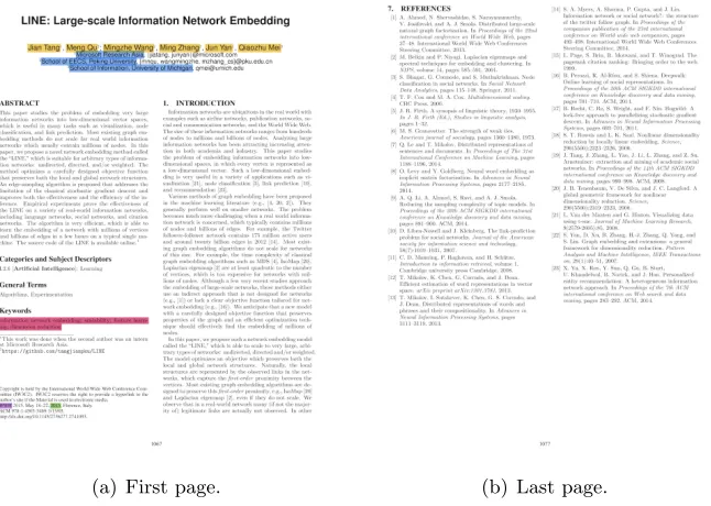
author(s), institution(s), publication year, and venue etc. Figure 1.1 shows a screenshot of

a paper. There are multiple entities on the first page as shown in Panel (a). After the main

content, including text, figures, and tables, the paper cites existing works as illustrated in

Panel (b). Thus, academic papers are more complex than pure documents with plain text

(21)

(a) First page. (b) Last page.

FIGURE 1.1: A screenshot of an academic paper. The first page in Panel (a) has multiple entities marked in different colors. Here authors are yellow, institutions are blue, keywords are red, venue is purple and publication year is green. This paper also links to other related papers via citation links as illustrated in Panel (b).

The complex structure of academic papers contains rich information. By studying

aca-demic papers, we can develop tools such as search engine to help scientists improve the

quality and productivity of their academic research. In fact, the industry has developed

services such as Google Scholar1 _{and Semantic Scholar}2_{. Measuring the similarity between}

authors and papers can also be very useful. By checking the similarity between authors,

we can design a search engine to help researchers find potential collaborators in the same

research field. The similar paper search engine can also be used to help researchers search

related works. Meanwhile, we can predict the influential researches by mining the scholarly

data, which can be used to help institutions and governments to follow the trend of the

science and technology and allocate the research fundings.

There are substantial works [Yang et al., 2018, M¨uller, 2017] using machine learning

techniques to extracting information from academic papers. Unlike humans, computers can

not understand the words, authors, or citations naturally. Therefore, we need to represent

the text and links in a way that computers can understand, which are vectors. This

(22)

dure is commonly known as data representation [Goodfellow et al., 2016]. Taking words as

an example, word representation is traditionally dealt with bag of words model [Manning

et al., 2010]. The bag of words model treats every word independently so that the similarity

between every two words are the same. Suppose we have three words ‘cat’, ‘dog’, and

‘com-puter’ in the vocabulary. The bag of words model uses binary vector to represent them. Let

the vector representations for them be (1,0,0), (0,1,0), and (0,0,1), respectively. Then for

any two words, the Euclidean distance between their representations is √2 and the cosine

similarity is 0. In natural language, words have semantic meanings. Thus, we can improve

the performance of Neural Language Models (NLM) by giving similar words similar

rep-resentations. It can be done by learning word embeddings using word2vec [Mikolov et al.,

2013b] algorithms. Different from the long sparse vectors, embeddings are short dense

vec-tors. They can be obtained by applying dimensionality reduction algorithms on the sparse

vectors [Yang et al., 2015, Zhang et al., 2016], or learned by embedding algorithms such as

word2vec [Mikolov et al., 2013b] for words, Paragraph Vector [Le and Mikolov, 2014] for

documents, or DeepWalk for networks [Perozzi et al., 2014].

1.2 Challenges

Representing academic papers is challenging. One issue is the large size of scholarly data.

It was estimated that there are hundreds of millions of academic papers [Khabsa and Giles,

2014], and at least 6,000 more are added to the stack everyday [Gibney, 2014]. As of the

end of 2018, ArnetMiner [Tang et al., 2008] contains 2.7 million papers in the domain of

Computer Science with 25 million citations. There are 46 million papers and 528 million

citation links in MAG (Microsoft Academic Graph) [Sinha et al., 2015]. The Health data,

which are provided by our industry parter 3, have 46 million papers, 13 million authors,

and 479 million citation links. Traditional methods are often computational expensive and

can not scale to large datasets. Therefore, an efficient method is needed to represent such

data.

The second challenge is that academic papers are complicated. They contain not only

plain text, such as titles and abstracts, but also link to each other through citations.

Repre-senting text has been widely studied in the past. Traditional techniques, such as n-grams and

(23)

Term Frequency-Inverse Document Frequency (TF-IDF) [Rajaraman and Ullman, 2011],

are widely used. However, these methods suffer from the high dimensionality problem. To

reduce the dimension of these representations, researchers have proposed various models,

such as Latent Dirichlet Allocation (LDA) [Blei et al., 2003] and Latent Semantic Analysis

(LSA) [Dumais, 2005]. However, these methods are computationally expensive [Cai et al.,

2008] and can not scale to large datasets. In 2013, Mikolov et al. [2013b] proposed skip-gram

with negative sampling model (hereafter SGNS) that can efficiently learn high-quality word

embeddings from a large corpus. It has the state-of-the-art performance and inspires many

algorithms to learn embeddings from different types of data. Le and Mikolov [2014] extend

word2vecto learn document embeddings and propose Paragraph Vector (PV). Meanwhile,

researchers apply different sampling strategies on SGNS to learn node representations from

networks, such as DeepWalk [Perozzi et al., 2014], LINE [Tang et al., 2015b], andnode2vec

[Grover and Leskovec, 2016].

Academic papers are more complicated than plain text or networks. Utilizing link

infor-mation in document representation has been studied in several ways. A naive method is to

train document embeddings from text and network embeddings from links independently,

then concatenate them together. Yang et al. [2015] propose Text-Associated DeepWalk

(TADW) that generates paper embeddings by factorizing the DeepWalk matrix with

TF-IDF matrix. Another approach treats texts and links equally by forming the data into a

heterogeneous network, then applies network embedding algorithms to retrieve the paper

embeddings [Wang et al., 2018, Ganguly and Pudi, 2017]. In 2016, Wang et al. [2016b]

propose LDE, a supervised model that can learn the embeddings from labeled linked

docu-ments. They split the data into three components and design the objective function for each

component. Then they optimize these multiple objectives together to get the embeddings

for labeled linked documents.

1.3 Contributions

This dissertation aims to learn high quality embeddings from academic papers. We

sum-marize our main contributions from five aspects:

• Norm convergence issue of SGNS: SGNS is the state-of-the-art word embedding

(24)

from different types of data such as networks [Perozzi et al., 2014, Tang et al., 2015b,

Grover and Leskovec, 2016], documents. We observed that the performance of SGNS

based network embedding algorithms degenerates over iteration. By monitoring the

training process of SGNS based network embedding algorithms, we show that SGNS

and its variants suffer from the norm convergence issue. This problem can be fixed

by adding a L2 regularization. We also verify our method on words and documents.

• Fast implementation for SGNS-based models: Our proposed methods are built

on top of SGNS. We re-implement the SGSN model from scratch using Python, Cython

and Basic Linear Algebra Subprograms (BLAS). Our implementation is optimized

for modern CPUs and is faster than most existing implementations [Mikolov et al.,

2013b, ˇReh˚uˇrek and Sojka, 2010, Ji et al., 2019]. The source code is available on

our webpagehttp://zhang18f.myweb.cs.uwindsor.ca/p2v.

• Network Embeddings: Most of the data in real-world are in the form of networks.

Thus, network embeddings algorithms are also covered in this dissertation. We

de-signed an author paper network (APN) to learn the embeddings for authors. Existing

methods are designed for undirected graphs. This dissertation addresses the problems

and solutions for directed graphs. We also propose a new network embedding

algo-rithm called N2V (network2vector). Experiment shows that N2V improves existing

methods and has state-of-the-art performance in many tasks.

• Document Embeddings: PV-DBOW (Paragraph Vector – Distributed

Bag-of-words) [Le and Mikolov, 2014] is one of the most widely used document embedding

algorithm. However, it does not capture word semantics directly in the training

pro-cess. Existing work suggests using pre-trained SGNS model can improve the quality

of document embeddings. We propose a novel method called D2V (document2vector)

to improve PV-DBOW with word semantics. In D2V, the word semantic relations

and document embeddings are learned simultaneously. The weights of words are

con-trolled by a hyper-parameter to suit different datasets. Experimental results show

that D2V can improve PV-DBOW on the classification task. We also show that word

meanings have different impacts on different types of datasets by examining the weight

(25)

• Paper Embeddings: There is limited research on learning the representation of linked documents such as academic papers. In this dissertation, we propose a new

neural network based algorithm, called P2V (paper2vector), to learn high-quality

embeddings for academic papers on large-scale datasets. We compare our model with

traditional non-neural network based algorithms and state-of-the-art neural network

methods on datasets of various sizes. The largest dataset we used contains 46.64

million papers and 528.68 million citation links. Experimental results show that P2V

achieves state-of-the-art performance in many tasks such as paper classification, paper

similarity, and paper influence prediction task.

• Applications: Academic papers contains rich information. In this dissertation, we

build four applications using embeddings techniques. We first propose author paper

network to learn embeddings for authors. Then we build a website to search similar

authors in Computer Science, where scientists can use our website to find the

poten-tial collaborators. The second application we build is a paper search engine for the

domain of Computer Science. Our search engine can find the most similar papers

in term of content and citations. Experimental results suggest our search engine has

higher accuracy than existing services such as Google Scholar and Semantic Scholar.

Embeddings generated from academic papers can be used as the input of subsequence

tasks. Therefore, we demonstrate how to use paper embeddings to solve real-world

problem such as author name disambiguation and paper influence prediction.

1.4 The structure of the dissertation

The rest of this dissertation is organized as follows. We first review the existing literature

in Chapter 2. It covers the related works and background knowledge from four aspects. 1)

Word embeddings. 2) Document embeddings. 3) Network embeddings. 4) Linked document

embeddings. Our proposed methods are based on SGNS model. Hence, we also introduce

the implementation details of SGNS.

Chapter 3 first proposes ShortWalk that improves DeepWalk in directed graphs. Then

it addresses the norm convergence issue in SGNS, which can be fixed by L2

regulariza-tion. Furthermore, it presents a new method N2V for network embeddings. Extensive

(26)

After that, we present a new document embedding method D2V in Chapter 4. Our D2V

improves PV-DBOW with word semantics and achieves the state-of-the-art performance in

most datasets.

The focus of this dissertation is learning embeddings for academic papers. In Chapter

5, we present P2V by combining D2V and N2V. We validate our model on seven datasets

with various sizes, where the largest one contains 46.6 million papers. Four applications are

proposed and discussed in Chapter 6, including author search engine, similar paper search

engine, author name disambiguation, and paper influence prediction. The conclusions of

(27)

Background and Related Works

This chapter discusses the background knowledge of embeddings. We first start with word

embeddings in Section 2.1. Then we introduce document embedding algorithms in Section

2.2. Section 2.3 and Section 2.4 review existing works for network and linked document

embeddings. The summary is in Section 2.5. Before going into the details, we summary

the notations used throughout this dissertation in Table 2.1.

2.1 Word embeddings

Representing words has been studied for many years. The most straightforward method

is to encode a word into a one-hot vector, where 1 indicates the index of the word in the

vocabulary. This method treats every word equally but ignores the relation between words.

However, word has semantic meanings which computers can not understand naturally. In

1996, Lund and Burgess [1996] found that the context of a word can reflect its semantic

meaning. Therefore, they propose to use the word-context co-occurrence matrix to represent

words. Recently, Mikolov et al. [2013b] propose word2vec that can learn word embeddings

from a large corpus. They capture the word-context co-occurrence information via a sliding

window where the closer context will have more weight than the further ones. Word2vec

learns the embeddings via a shallow neural network. It has two models – Continuous

Bag-of-Words Model (CBOW) and Skip-gram with negative sampling Model (SGNS). CBOW

takes the average of context words representations to predict the center word, while SGNS

takes the embedding of a word to predict its context. The experiments show that word2vec

(28)

TABLE 2.1: Summary of the notations.

Notation Meaning

v Embedding vector

u Output vector

d Dimension of the embeddings

w Window size

λ Weight of regularization

η Learning rate

di i-th paper/document in a dataset

ni i-th node in a graph

wi i-th word in a dataset/corpus

V Vocabulary

N Number of documents

T Length of corpus

S Number of training pairs

K Number of negative samples

Pn Noise distribution

kx_k2 L2 norm of vectorx

σ(·) Sigmoid function σ(x) =_1+exp(1 ₋_x₎

Ex∼Pf(x) Expectation of f(x) with respect toP(x)

from word2vec, Pennington et al. [2014] propose Global Vectors for Word Representation

(GloVe), which generates word embeddings by factorizing the word-word co-occurrence

matrix. These works are proved as a variant of factorization over a specific matrix [Levy

and Goldberg, 2014], i.e., SGNS is implicitly factorizing a shifted weighted Pointwise Mutual

Information matrix (PMI), and GloVe is factorizing the biased word-context co-occurrence

count matrix. Experiments [Baroni et al., 2014, Levy et al., 2015] show that the

predict-based models such as SGNS are superior to the count-predict-based model (GloVe).

2.1.1 Co-occurrence matrix

Word co-occurrence has been widely applied for capturing the word semantic meanings in

word representation. The simplest way is to use the raw count of the word co-occurrence.

Figure 2.1 and Table 2.2 show an example. Suppose we have a corpus that consists a set

of words in a specific order _{w1, w2, w3, w4, w5, w6, w7, w8, w9}, when the window size is 5,

we move the window from left to right over the corpus. The window captures five words

at each time. For every pair of the words occurred in that window, we add the count for

(29)

w

1

w

2

w

3

w

4

w

5

w

6

w

7

w

8

w

9

position=1

w

1w2

w

3

w

4

w

5

w

6w7

w

8

w

9

position=2

w

1

w

2

w

3

w

4

w

5

w

6

w

7

w

8

w

9

position=3

w

1

w

2

w

3w4

w

5

w

6

w

7

w

8w9

position=4

w

1

w

2

w

3

w

4

w

5

w

6

w

7

w

8

w

9 position=5

FIGURE 2.1: An example of a basic sliding window when capturing word-context co-occurrence information. The corpus is a set of words in a specific order. Suppose window

sizeC= 5, the window moves from left to right and captures 5 words at each time. Every

two words appeare in that window count as one occurrence. We can record the co-occurrence count in a matrix listed in Table 2.2.

c1 c2 c3 c4 c5 c6 c7 c8 c9

w1 0 1 1 1 1 0 0 0 0

w2 1 0 2 2 2 1 0 0 0

w3 1 2 0 3 3 2 1 0 0

w4 1 2 3 0 4 3 2 1 0

w5 1 2 3 4 0 4 3 2 1

w6 0 1 2 3 4 0 3 2 1

w7 0 0 1 2 3 3 0 2 1

w8 0 0 0 1 2 2 2 0 1

w9 0 0 0 0 1 1 1 1 0

TABLE 2.2: The word-context co-occurrence matrix retrieved from Figure 2.1. Row i

denotes word wi and columnj is context cj. Each entry Mi,j is the co-occurrence between

wordwi and contextcj, which is the count ofwi andcj appears in the same sliding window.

each row i corresponds to word wi and each column j represent a context cj. When the

window reaches to the end of the corpus, we will have a word-context co-occurrence matrix

M. Each entryMi,j is the frequency ofwi andcj appears in the sliding window.

This method and its variants are widely applied to capture the word semantic meanings.

For example, in Hyperspace Analogue to Language (HAL) [Lund and Burgess, 1996], the

authors move a sliding window on the corpus and calculate the weighted count of each word

pair presented in that window. They test the similarities between the word representations

by analyzing the nearest neighbors of a set of words. They also visualize the embeddings

and demonstrate the words categories. However, HAL uses the raw count of the words in

the co-occurrence matrix so that the weight of the words is generally large. COALS [Rohde

et al., 2006] further improves HAL by replacing the raw count with Pearson’s correlation

(30)

test COALS on 17 datasets and observed significant improvement (overall 148.92%) over

HAL.

The existing works give us a good overview of the effectiveness of word co-occurrence

matrix [Lund and Burgess, 1996, Jarmasz and Szpakowicz, 2004, Rohde et al., 2006]. Yet,

the efficiency of generating such representation remains an issue. In a real-world dataset,

the corpus is usually large, resulting to a large vocabulary. In the co-occurrence matrix, each

row represents a word in that vocabulary. Therefore, the size of the co-occurrence matrix

will be huge. Despite the matrix is sparse, building such a matrix is still computationally

expensive. The dimension of the word representation is also large, making it hard to apply to

downstream applications such as classification, clustering, recommendation etc. Therefore,

it is common to see researchers such as Rohde et al. [2006] to apply dimensional reduction

techniques such as SVD (Singular Value Decomposition) [Manning et al., 2010] to transform

the long sparse representation into short dense vectors – embeddings.

2.1.2 Word2vec

Word2vec is a set of models proposed by Mikolov et al. [2013b]. It has two models –

Contin-ues Bag-of-words (CBOW) and Skip-Gram with Negative Sampling (SGNS). Embeddings

generated by word2vec have many advantages compared to traditional methods [Mikolov

et al., 2013a] and can easily scale to large corpus with billions of words. These algorithms

take a large corpus as input and produces dense d-dimensional vectors where each word is

assigned to a unique vector in that vector space. The similarity between two words can be

measured by cosine similarity defined as

similarity(A,B) = A·B

kA_kkB_k =

n P i=1

AiBi

s n P i=1

A2

i s

n P i=1

B2

i

, (2.1)

whereAi and Bi are elements of n-dimensional vectorsA and B. In word2vec, the spatial

distance between two embeddings corresponds to the word similarity. For example, the

similarity between embeddings of Canada and China is larger than the similarity between

embeddings of Canada and cheese. Moreover, the displacement between two words

rep-resents the word relationship. For example, the distance between Canada and China is

(31)

w

1

w

2

w

3

w

4

w

5

w

6

w

7

w

8

w

9

iteration=1,c=randint(C)=2

w

1

w

2

w

3

w

4

w

5

w

6

w

7

w

8

w

9

w

1

w

2

w

3

w

4

w

5

w

6

w

7

w

8

w

9

w

1

w

2

w

3

w

4

w

5

w

6

w

7

w

8

w

9

FIGURE 2.2: An example of skip-gram window in word2vec. The corpus is a set of words

in a specific order. Let C = 4 be the window size, w5 be the center word, which is the

target word we want to learn the embedding for in this example. Function randint(C)

returns a random integer in a range of (0, C). In each iteration, we generate a window size

c = randint(C) and collect the (word,context) pairs within the window. For example, in

the third iteration, c is 1, we take 1 neighbor left and right to the center word w5. The

(word,context) pairs generated in this step is (w5, c4),(w5, c6).

w1 w2 w3 w4 w5 w6 w7 w8 w9

w5 1 2 3 4 0 4 3 2 1

TABLE 2.3: The word-context co-occurrence for w5 retrieved from Figure 2.2.

the words. For instance, when knowing the capital of China is Beijing, we can infer the

capital of Canada by calculating the most similar word embeddings to Beijing - China +

Canada.

Skip-gram window

The semantic meaning of a word relates to its neighbors in the corpus, also known as

context. Context with further distance is usually less related to the current word. Based on

this assumption, word2vec captures the word-context co-occurrence using a sliding window

c, wherecis a random integer in a range of (0, C) [Mikolov et al., 2013a]. Figure 2.2 shows an

example of this process. Suppose we have a corpus _{w1, w2, w3, w4, w5, w6, w7, w8, w9} and

the window sizeCis 5, our goal is to capture the context for wordw5. In the first iteration,

the skip-gram window size c is 2, so we take two context left tow5, and two context right

tow5. The window size is generated randomly in each iteration. After four iterations, the

word-context co-occurrence information for w5 is (1,2,3,4,0,4,3,2,1) as shown in Table

(32)

w

1

w

2

w

3

w

4

w

5

w

6

w

7

w

8

w

9

(a) Capture context for wordw5.

w

5

, w

3

, w

4

, w

6

, w

7

(b) Training sample derived from (a).

Input Layer

Hidden Layer

Output Layer

w1 0

w2 0

w3 1

w4 1

w5 0

w6 1

w7 1

w8 0

w9 0

h1

h2

hd

...

w1 0.10 0

w2 0.05 0

w3 _0.11 ₀

w4 0.20 0

w5 0.95 1

w6 0.24 0

w7 0.14 0

w8 0.05 0

w9 0.20 0

predict

label labeltrue

error Back Propagation

(c) Training procedure.

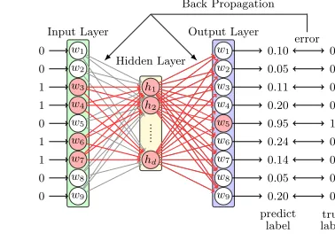
FIGURE 2.3: CBOW as Neural Network with one hidden layer.

Continues Bag-of-words (CBOW)

The first model proposed in word2vec is Continues Bag-of-words, also known as CBOW.

Given a corpus, the context of a word provides the information that defines the semantic

meaning of this word. For example, in the sentence “a cat sits on the mat”, the semantic

meaning of “sit” is defined by its context “a, cat, on, the, mat”. Based on this assumption,

word2vec learns embeddings by using the average/summation of the context representations

to predict the missing word. The authors name this model as Continues Bag-of-words, also

known as CBOW. Figure 2.3 shows an example. For each word in the corpus, w5 for

ex-ample, CBOW uses skip-gram window to capture the context (w3, w4, w6, w7) as illustrated

in Panel (a). Then it generates the training sample as shown in Panel (b). CBOW can be

explained as a shallow neural network with one hidden layer as illustrated in Panel (c). It

averages or sums the contexts’ embeddings into the hidden layer. In our example, the

in-put is (0,0,1,1,0,1,1,0,0), which sums the embeddings of context (w3, w4, w6, w7) into the

hidden layer. Then the model predicts the missing wordw5 with softmax function. For

ex-ample, the predict label from output layer is (0.10,0.05,0.11,0.2,0.95,0.24,0.14,0.05,0.20),

where each element is the probability of the corresponding word as the output. We can

see that there is an error between the predicted label and true label. Then we update

Neural Network weights using this error via back propagation algorithm. After optimizing

(33)

w1 0

w2 0

w3 0

w4 0

w5 1

.... w9

0

(a) Softmax

θ1

θ2

θ3

w2

w4 w6 w5 w3

w1 w9 w7 w8

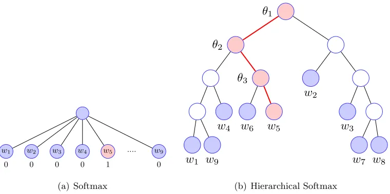
(b) Hierarchical Softmax

FIGURE 2.4: Comparison between Softmax and Hierarchical Softmax. Panel (a) illustrates the multi-class classification using Softmax. Panel (b) shows the Hierarchical Softmax. It solves the multi-class classification problem via multiple binary classifiers where labels are

the binary code of the target on the Huffman tree. In this example, w5 is the target word

and the corresponding binary code on the Huffman tree is (1,0,0).

embeddings. More formally, the objective function of CBOW is

O =1

T T X

i=1

logp(wi|wi−c, ..., wi+c), (2.2)

whereT is the length of the corpus,cis the window size,p(wj|wi−c, ..., wi+c) is the

probabil-ity of giving the average/summation of a set of words (wi−c, ..., wi+c) that observes context

wi. It is defined by the softmax function:

p(u_|v) = _P_Vexp(u·v)

n=1exp(u·v)

, (2.3)

where V is the size of the vocabulary. v is the embedding of the input word and u is the

output vector of the context.

However, calculating the softmax function directly is not practical due to the large

vocabulary size V. For example, the smallest dataset we have is Text81 [Mahoney, 2011].

The corpus size is 17,005,207 and the vocabulary size is 253,854. Such a small dataset

will generate about 17 million training samples. Applying softmax function will need to

calculate exp(u_·v) 17,005,207_×253,854 = 4.3_×1012 times per iteration. To reduce

1

(34)

w

1

w

2

w

3

w

4

w

5

w

6

w

7

w

8

w

9

(a) Capture context for wordw5.

w5, w3

w5, w4

w5, w6

w5, w7

(b) Training sample derived from (a).

Input Layer

Hidden Layer

Output Layer

w1

0

w2

0

w3

0

w4

0

w5

1

w6

0

w7

0

w8

0

w9

0

h1

h2

hd

...

w1 0.10 0

w2 0.05 0

w3 0.11 0

w4 0.95 1

w5 0.21 0

w6 0.24 0

w7 0.14 0

w8 0.05 0

w9 0.20 0

predict

label labeltrue

error Back Propagation

(c) Training procedure.

FIGURE 2.5: SGNS as Neural Network with one hidden layer.

the computation time, the authors use Hierarchical Softmax (HS) proposed by Mnih and

Hinton [2009] to replace softmax. More specifically, the output layer in Figure 2.3 Panel(c)

is replaced as a binary Huffman tree. The tree is built based on the word frequency, where

each leaf represents a word. In this binary Huffman tree, the more frequent a word is, the

faster we can reach it. Then, we can convert the multi-class classification problem into a

multiple binary classification problem where the output is the binary code of the target as

demonstrated in Figure 2.4. In this example, we use vectorvto predictw5. Panel (a) treats

this procedure as a multi-class classification problem that has nine outputs, wherew5 is 1

and others are 0. In Panel (b), HS treats it as three binary classification problems. The

expected outputs are (1,0,0), which are the Huffman binary code from root to w5. More

specifically, HS trains three binary classifiers. Each classifier has its own parameters. For

example, the root classifier has parameter θ1 and the expected output is 1. The second

classifier has parameterθ2and the expected output is 0. HS reduces the time complexity of

Softmax function exponentially – fromO(n) toO(log₂n). The difference is more significant

in NLP tasks where the vocabulary size is usually large.

Skip-gram with Negative Sampling (SGNS)

Another model proposed in word2vec is Skip-gram with Negative Sampling, also known as

SGNS. It has the state-of-the-art performance [Baroni et al., 2014]. It first captures the

word-co-occurrence information as word-context pairs. Figure 2.5 is an example. Panel

(35)

w1

0

w2

0

w3

0

w4

1

w5

0

.... w9

0

(a) Softmax

w1

0

w2 w3

0

w4

1

w5 .... w9

(b) Negative Sampling

FIGURE 2.6: Comparison between Softmax and Negative Sampling. Panel (a) illustrates the multi-class classification using Softmax. Panel (b) shows the Negative Sampling in which the negative samples are retrieved randomly via noise distribution.

we first capture the context for w5 with skip-gram window introduced in Section 2.1.2.

The corresponding training samples are [(w5, w3),(w5, w4),(w5, w6),(w5, w7)]. Panel (c)

shows the training process. For training sample (w5, w4), we take the embedding of w5

to predict the context representation of w4. More formally, given a sequence of training

corpus_{w1, w2, ..., wT}, the objective function is maximizing the average log probability of

all observed (word,context) pairs:

O= 1

S T X

i=1

X

−c≤j≤c,j6=0

logp(wi+j|wi), (2.4)

where S is the total number of observed training pairs, T is the length of the corpus, c is

the window size. p(wj|wi) is the probability of giving a word wi that observes context wj,

which is defined using softmax function:

p(wj|wi) = _PVexp(uwj·vwi)

n=1exp(uwn·vwi)

. (2.5)

Herewj is the context andwi is the word,vwi is the vector representation ofwi and uwj is

the vector representation of contextwj,V is the size of the vocabulary.

To reduce the computation time, the authors propose Negative Sampling (NS) to replace

the softmax function. Instead of calculating over the entire vocabulary, NS drawsknegative

samples according to a noise distribution Pn. Figure 2.6 shows a comparison between

Softmax and NS. Panel (a) is the softmax multi-class classification. It takes one vector as

the input and produces multiple output values. Each value represents the probability of the

(36)

input, NS in Panel (b) has only one output. Additional to the true labelw5 provided in the

training sample, NS also drawsknegative samples via a noise distributionPn, which arew1

andw3 in this example. Then the model can learn from these negative samples by treating

them as false labels. Intuitively, NS simplifies the multi-class classification problem into a

binary classification problem on a small sample. It uses the embedding of the observed word

to distinguish the observed context (true) and knegative samples (false) drawn according

the noise distribution Pn. The authors choose the word frequency raises to 3₄ as the noise

distribution:

Pn(w) = U(w)

3/4

Z (2.6)

whereU(w) denotes unigram distribution of wordw,Z =P

w∈V U(w)3/4 denotes the

nor-malization term. This noise distribution reduces the possibility of choosing a frequent word

as the negative sample, and is used in most related works and implementations [Mikolov

et al., 2013a,b, ˇReh˚uˇrek and Sojka, 2010]. Therefore, the local objective function for an

observed training pair (wi, wj) is:

logσ(uwj ·vwi) +

K X

k=1

Ewk∼Pnlogσ(−uwk ·vwi). (2.7)

Here,σ(x) = _1+exp(1 ₋_x₎ is the sigmoid function. K is the number of negative samples. v is

the embedding vector and u is the context vector.

Existing works use Stochastic Gradient Descent (SGD) to optimize the local objective

function for each observed training pair [Mikolov et al., 2013b]. The gradient is calculated by

Back propagation, which is commonly used by the gradient descent optimization algorithm

to adjust the weight by calculating the gradient of the loss function [Goodfellow et al., 2016].

Given a specific training pair (wi, wj), the derivative of Eq 2.7 regarding to the word vector

vwi is:

∂O(wi, wj)

∂wi

=∂{logσ(uwj·vwi) +

PK

k=1Ewk∼Pn[logσ(−uwk·vwi)]}

∂vwi

=∂logσ(uwj ·vwi)

∂vwi

+

K X

k=1

Ewk∼Pn

∂logσ(−uw_k ·vwi)

∂vwi

(37)

It can be rewritten into

∂O(wi, wj)

∂wi

=∂logσ(uwj·vwi)

∂σ(uwj·vwi)

·∂σ_∂u(uwj·vwi)

wj·vwi

·∂uw_∂vj·vwi

wi

+

K X

k=1

Ewk∼Pn

∂logσ(₋uwk·vwi)

∂σ(−uw_k·vw_i) ·

∂σ(₋uwk·vwi)

∂−uw_k·vw_i ·

∂₋uwk·vwi

∂vw_i

(2.9)

Since ∂log(_∂xx) = _x1, ∂σ_∂x(x) =σ(x)_·(1₋σ(x)), and ∂a_∂x·x =a, the above formula falls into

∂O(wi, wj)

∂wi

= 1

σ(uwj·vwi)

·σ(uwj ·vwi)(1−σ(uwj·vwi))·uwj

+

K X

k=1

Ewk∼F req(u)

1

σ(₋uwk·vwi)

·σ(₋uwk·vwi)(1−σ(−uwk·vwi))· −uwk

(2.10)

We can simplify it into

∂O(wi, wj)

∂wi

=(1−σ(uwj ·vwi))·uwj +

K X

k=1

Ewk∼Pn−(1−σ(−uwk·vwi))·uwk

=(1−σ(uw_j ·vw_i))·uw_j +

K X

k=1

Ewk∼Pn−(1−(1−σ(uwk·vwi)))·uwk

=(1−σ(uwj ·vwi))·uwj +

K X

k=1

Ewk∼Pn−σ(uwk ·vwi)·uwk

(2.11)

Similarly, for a specific observed pair (wi, wj), the derivative of Eq2.7 regarding to the

context word wj is:

∂O(wi, wj)

∂wj

PK

k=1Ewk∼Pn(w)[logσ(−uwk·vwi)]}

∂uwi

=∂logσ(uwj·vwi)

∂uwj

=∂logσ(uwj·vwi)

∂σ(uwj ·vwi)

·∂σ(uwj·vwi)

∂uwj·vwi

·∂uwj·vwi

∂uwj

= 1

σ(uwj·vwi)

·σ(uwj·vwi)(1−σ(uwj·vwi))·vwi

=(1₋σ(uwj ·vwi))·vwi

(38)

For a specific observed pair (wi, wj), the derivative of Eq2.7 regarding a negative sampling

context word wk is:

∂O(wi, wj)

∂wk

PK

k=1Ewk∼Pn(w)[logσ(−uwk·vwi)]}

∂uwk

=∂logσ(−uwk ·vwi)

∂uwk

=∂logσ(−uwk ·vwi)

∂σ(₋uwk·vwi)

·∂σ(−uwk ·vwi)

∂₋uwk·vwi

·∂−uwk·vwi

∂uwk

= 1

σ(−uw_k·vw_i) ·σ(−uwk·vwi)(1−σ(−uwk·vwi))· −vwi

=(1−(1−σ(uw_k·vwi)))· −vwi

=−σ(uw_k·vwi)·vwi

(2.13)

Moreover, we can summarize the derivative of context wj and negative samplewk into

(t₋σ(uwj·vwi))·vwi (2.14)

wheret= 1 whenwj is a context andt= 0 whenwj is a negative sample. Thus, the update

equations for SGNS model are:

vwi ←vwi+η[(1−σ(uwj·vwi))·uwj+

K X

k=1

Ewk∼Pn−σ(uwk·vwi)·uwk]

uwj ←uwj +η[t−σ(uwj·vwi)·vwi],

(2.15)

where t = 1 when wj is a context word, and t = 0 when wj is a negative sample. η is

the learning rate, which decays linearly from 0.025 to 0.0001 in most related works and

implementations [ ˇReh˚uˇrek and Sojka, 2010, Mikolov et al., 2013b, Tang et al., 2015b,

Goyal and Ferrara, 2018].

In theory, Levy and Goldberg [2014] proved SGNS implicitly factorizes a weighted shifted

word-context PMI (Pointwise Mutual Information) matrix M. In this matrix, row i

cor-responds to word wi and column j corresponds to context cj. Each entry of Mi,j is the

Pointwise word-context co-occurrence log P(wi,cj)

(39)

of an item, then we have:

#(w) = X

c∈Vc

#(w, c)

#(c) = X

w∈Vw

#(w, c)

(2.16)

We first begin with rewriting SGNS into:

X

w∈Vw

X

c∈Vc

#(w, c) [logσ(w~_·~c) +k_·EcN∼Pnlogσ(−w~·~cN)]

= X

w∈Vw

X

c∈Vc

#(w, c) logσ(w~ ·~c) + X

w∈Vw X

c∈Vc

#(w, c) [k·EcN∼Pnlogσ(−w~ ·~cN)]

(2.17)

w is word, c is context, w~ and ~c is the corresponding vector representation, Vw and Vc is

the word context vocabulary respectively

According to Eq 2.16, it equals to:

X

w∈Vw X

c∈Vc

#(w, c) logσ(w~·~c) + X

w∈Vw

#(w) [k·EcN∼Pnlogσ(−w~ ·~cN)] (2.18)

When using unigram distribution as the noise distribution, we can write the negative

sampling part into

EcN∼Pnlogσ(−w~·~cN)

= X

cN∈Vc

#(cN)

T logσ(−w~·~cN)

=#(c)

T logσ(−w~·~c) +

X

cN∈Vc\{c}

#(cN)

T logσ(−w~·~cN)

(2.19)

here T is the size of corpus. Combining Eq 2.18 and 2.19, then the local objective for a

specific (w, c) pair is

#(w, c)·logσ(w~·~c) +k·#(w)·#(c)

(40)

To optimize the objective, we definex= (w~ _·~c) and take the derivative of Eq 2.20

#(w, c)_·σ(₋x)₋k_·#(w)_·#(c)

T ·σ(x) (2.21)

Let the derivative equals to zero, we will have

e2x₋ #(w, c)

k·#(w)·#(_Tc) −1

!

ex₋ #(w, c)

k·#(w)·#(_Tc) = 0 (2.22)

And the only valid solution is

x=w~ ·~c= log

#(w, c)·T

#(w)_·#(c)

−logk

= log

#(w,c)

T

#(w)

T ·

#(c)

T !

−logk

= log P(w, c)

P(w)·P(c) −logk

(2.23)

Thus, SGNS factorizes this matrixMinto embeddings matrixV_|_V_|×_dand context matrix

U_|_V_|×_d, e.g.

M_⇒V_×U>

2.1.3 Implementation details of SGNS

SGNS has the state-of-the-art performance and can easily adopts to large datasets. This

dissertation focuses on learning embeddings for different types of data. Therefore, it is

necessary to have an efficiency and accuracy implementation of SGNS. In this work, we

reimplemented SGNS from scratch using Python, Cython and Basic Linear Algebra

Sub-programs (BLAS). Python is an interpreted, high-level, general-purpose programming

lan-guage. Benefit from the rich third-party libraries, it is widely used for researchers and

scientists to quickly develop, verify and analyze their ideas. Cython is an optimizing static

compiler for both the Python programming language and the extended Cython

program-ming language. It allows users to write C/C++ extensions for Python for better

perfor-mance. Optimizing SGNS requires extensive vector computation. BLAS provides common

linear algebra operations such as dot production, matrix multiplication. These functions

(41)

Algorithm 1 SGNS

1: function_SGNS(corpusT, window sizeC, learning rateη, number of negative samplesK, embeddings

dimensiond, word min countmin, subsampling thresholdt)

2: Generate the vocabularyV fromT

3: Calculate the word distributionP fromT

4: TrimV with word min countmin

5: forwordwi in vocabularyV do

6: Initializevwi←uniform(−

0.5 d ,

0.5

d ) for each dimension ofvwi

7: Initializeuwi←0 for each dimension ofuwi

8: Calculate subsampling probabilitypwi =max(0,1−

q

t P(wi))

9: Calculate noise distributionPn(wi) = P(wi)

0.75 P

wj∈VP(wj)0.75

10: end for

11: foreach iterationdo

12: fornext wordwi in corpusT do

13: Windowc←random integer∈(0, C)

14: foreach contextwjcaptured by windowcdo

15: if pwi<uniform(0,1)then

16: Update context vectoruwj according to Eq. 2.15

17: Drawk negative samples according to noise distributionPn.

18: foreach negative samplewkdo

19: Update context vectoruwk according to Eq. 2.15

20: end for

21: Update embedding vectorvwi according to Eq. 2.15

22: Decay learning rateη

23: end if

24: end for

25: end for

26: end for

27: returnembeddingsv