Development of a Regional Structured and Unstructured Grid Methodology for Chemically Reactive Turbulent Flows.

ABSTRACT

STEFANSKI, DOUGLAS LAWRENCE. Development of a Regional Structured and Unstructured Grid Methodology for Chemically Reactive Turbulent Flows. (Under the direction of Drs. Jack R. Edwards and Hong Luo).

A finite volume method for solving the Reynolds Averaged Navier-Stokes (RANS) equations on unstructured hybrid grids is presented. Capabilities for handling arbitrary mixtures of reactive gas species within the unstructured framework are developed. The modeling of turbulent effects is carried out via the 1998 Wilcox model. This unstructured solver is incorporated within VULCAN – a multi-block structured grid code – as part of a novel patching procedure in which non-matching interfaces between structured blocks are replaced by transitional unstructured grids. This approach provides a fully-conservative alternative to VULCAN’s non-fully-conservative patching methods for handling such interfaces.

Development of a Regional Structured and Unstructured Grid Methodology for Chemically Reactive Turbulent Flows

by

Douglas Lawrence Stefanski

A dissertation submitted to the Graduate Faculty of North Carolina State University

in partial fulfillment of the requirements for the degree of

Doctor of Philosophy

Aerospace Engineering

Raleigh, North Carolina 2013

APPROVED BY:

_______________________________ ______________________________

Dr. J. R. Edwards Dr. H. Luo

Committee co-Chair Committee co-Chair

________________________________ Dr. H. Hassan

DEDICATION

BIOGRAPHY

Douglas Stefanski was born on October 27, 1984 in Ithaca, New York. Shortly thereafter, his family moved to Cary, North Carolina, where he spent his youth. He graduated from Cary High School in 2003 and enrolled at North Carolina State University. There he developed an interest in computational fluid dynamics while pursuing BS degrees in aerospace engineering and applied mathematics. Upon graduation in 2008, Doug was accepted into the ‘en route’ PhD program in aerospace engineering at NCSU and began work under the direction of Drs. Edwards and Luo. During this time he was awarded a GAANN (Graduate Assistance in Areas of National Need) Fellowship and participated in the NCSU Preparing the Professoriate mentored teaching program. Doug earned his MS in aerospace engineering in 2010 and has continued working toward his PhD since.

ACKNOWLEDGMENTS

I would first like to thank my advisors, Drs. Edwards and Luo, for their guidance and support throughout my graduate career. I would also like to thank Drs. Hassan, Kelley and Samatova for their service on my committee.

Thanks to my fellow students and coworkers, and in particular, thanks to Seth Spiegel for his collaboration on the FVFLO-NCSU/VULCAN development.

This work was carried out under NASA contract NNL08AA22C. Special thanks to Jeffery White, Rob Baurle, and the Hypersonic Airbreathing Propulsion Branch of NASA Langley Research Center.

Thanks to the GAANN Fellowship Program at NCSU for providing support for my research and education. Thanks also to Dr. Melissa Bostrom and all the other faculty and presenters involved with the Preparing the Professoriate program.

Thanks to the NCSU Office of Information Technology for providing HPC resources used in this work.

TABLE OF CONTENTS

LIST OF TABLES ... vii

LIST OF FIGURES ... viii

NOMENCLATURE ... xi

Chapter 1: Introduction ... 1

Chapter 2: Governing Equations ... 10

2.1 Navier-Stokes Equations ... 10

2.2 Reynolds-averaged Navier-Stokes Equations ... 15

Wilcox (1998) - Two-Equation Model ... 20

Wall Matching ... 22

2.3 Filtered Navier-Stokes Equations ... 26

Chapter 3: Numerical Methods ... 29

3.1 Finite Volume Method ... 29

3.2 Flux Discretization ... 31

Inviscid Fluxes ... 31

Viscous Fluxes ... 34

Second-Order Extension ... 35

Ducros Blending ... 36

3.3 Time Integration ... 38

Steady-State ... 38

Time accuracy ... 47

Chapter 4: Hybrid Coupling... 49

4.1 Structured/Unstructured Solver Integration ... 49

4.2 Unstructured Patching ... 50

Chapter 5: Hybrid Solver Results ... 51

Reacting Inviscid Supersonic Flow into a 15 Compression Corner (I)... 51

Laminar Low Reynolds Number Flow Past a Sphere ... 55

Reacting Laminar Viscous Flow over a Flat Plate ... 57

Supersonic Turbulent Flow over a Flat Plate ... 60

Supersonic Turbulent Flow over a Flat Plate with Wall Matching ... 64

Supersonic Turbulent Reactive Flow over a Zero-Thickness Splitter Plate ... 67

Turbulent Rectangular-to-Elliptical Shape Transition Scramjet Inlet ... 69

Hybrid VULCAN/FVFLO-NCSU Results ... 75

Reacting Inviscid Supersonic Flow into a 15 Compression Corner (II) ... 75

Inviscid Supersonic Flow over Two Bumps in a Channel ... 78

Laminar Supersonic Flow over a Flat Plate ... 83

5.3 FVFLO-NCSU LES Results ... 87

Confined Supersonic Mixing Layer ... 87

Chapter 6: Summary and Conclusions ... 97

LIST OF TABLES

Table 2.1: Model Constants ... 22

Table 3.1: Multi-stage Runge-Kutta coefficients ... 40

Table 5.1: NASA Langley 7 species/7 reaction H2-air kinetic model ... 52

Table 5.2: Confined mixing layer inflow parameters ... 88

LIST OF FIGURES

Figure 1.1: Sketch of Cartesian grid near solid boundary ... 2

Figure 1.2: Multiblock meshes: (a) overset, (b) patched, (c) composite ... 5

Figure 3.3: Sketch of neighboring cells for gradient computation ... 34

Figure 4.1: Hybrid patching procedure ... 50

Figure 5.1: Mesh for supersonic reacting inviscid flow into 15 compression corner ... 53

Figure 5.2: Temperature and OH mass fraction contours for compression corner ... 53

Figure 5.3: OH mass fraction profile along gridline y = 0.3 and Temperature profile about gridline x = 0.5 ... 54

Figure 5.4: Unstructured mesh for low Reynolds number sphere ... 55

Figure 5.5: Streamlines for laminar flow past a sphere computed by FVFLO-NCSU ... 56

Figure 5.6: Parallel speedup for the laminar sphere ... 57

Figure 5.7: Mach number predictions for reacting laminar flow over a flat plate ... 58

Figure 5.8: Temperature and H2O mass fraction predictions ... 59

Figure 5.9: Three grids for supersonic turbulent flow over a flat plate ... 61

Figure 5.10: Outlet profiles of -velocity for supersonic turbulent flat plate ... 62

Figure 5.11: Outlet profiles of temperature for supersonic turbulent flat plate ... 62

Figure 5.12: Outlet profiles of turbulent kinetic energy for supersonic turbulent flat plate ... 63

Figure 5.13: Outlet profiles of for supersonic turbulent flat plate ... 63

Figure 5.14: Outlet profiles of -velocity for wall matching flat plate ... 65

Figure 5.15: Outlet profiles of temperature for wall matching flat plate ... 65

Figure 5.18: Mesh for supersonic reacting splitter flow ... 67

Figure 5.19: Splitter plate temperature contours ... 68

Figure 5.20: Splitter plate outlet boundary profiles. H2O mass fraction (left) and eddy viscosity ratio (right) ... 68

Figure 5.21: Configuration of modular REST inlets ... 70

Figure 5.22: Computational mesh for REST inlet ... 70

Figure 5.23: REST inlet symmetry plane contours ... 72

Figure 5.24: REST inlet cross-section contours ... 73

Figure 5.25: Parallel speedup for the REST inlet ... 74

Figure 5.26: Hybrid mesh for supersonic compression corner ... 76

Figure 5.27: Contour plots for hybrid reacting wedge ... 77

Figure 5.28: Bumps in channel mesh for the patch-y and hybrid-yz cases ... 79

Figure 5.29: Unstructured patch for hybrid-y and hybrid-yz cases ... 80

Figure 5.30: Solution contours for patch-y and hybrid-y cases ... 81

Figure 5.31: Solution contours for patch-yz and hybrid-yz cases ... 82

Figure 5.32: Residuals for the two bumps in a channel test cases ... 83

Figure 5.33: Grids for the flat plate patched and hybrid cases ... 84

Figure 5.34: Unstructured patch for the hybrid flat plate case ... 85

Figure 5.35: Solution contours for the laminar flat plate ... 86

Figure 5.36: Residual convergence for the patched and hybrid laminar flat plate ... 87

Figure 5.37: Zoomed views of structured and unstructured grids for mixing layer ... 89

Figure 5.38: Confined mixing layer H2 mass fraction contours ... 90

Figure 5.40: Mean flow profiles for -velocty, temperature, and H2 mass fraction two

axial stations: m and m ... 92 Figure 5.41: H2O mass fraction and temperature contours for constrained mixing

layer ... 95 Figure 5.42: H2O mass fraction and temperature contours, Chakraborty, et al. ... 95 Figure 5.43: Mean flow profiles at from Chakraborty, et al. with

NOMENCLATURE Roman Letters

speed of sound

thermodynamic curve fit constants Arrhenius equation prefactor

species concentration turbulence model constant

specific heat at constant pressure specific heat at constant volume Smagorinsky coefficient

diagonal matrix

laminar species diffusion internal energy per unit mass total energy per unit mass inviscid flux vector species Gibbs free energy viscous flux vector

total change in Gibbs free energy for a reaction enthalpy per unit mass

total enthalpy per unit mass

turbulent kinetic energy

MUSCL interpolation parameter thermal conductivity

reaction rate coefficients lower triangular matrix

_{sums of reactant and product stoichiometric coefficients}

Mach number molecular weight static pressure

time-averaged or filtered static pressure

Prandtl number unknown variable heat flux vector

residual vector unsteady residual specific gas constant universal gas constant

Reynolds number

strain-rate tensor

Schmidt number time

static temperature

laminar stress tensor

x-direction component of velocity velocity vector

friction velocity

vector of conserved variables upper triangular matrix cell-interface variables

y-direction component of velocity velocity vector

volume

z-direction component of velocity direction vector

Greek Letters

turbulence model constant turbulence model constant turbulence model constant control volume surface area forward difference operator backward difference operator

Kronecker delta

a small number reaction activation energy Arrhenius equation constant

surface normal coordinate direction von Karman’s constant

eigenvalue

molecular viscosity eddy viscosity kinematic viscosity

_{stoichiometric reaction coefficients}

surface tangent coordinate direction density

turbulence model constant turbulence model constant

stress tensor

specific dissipation rate of turbulence kinetic energy

̇ species source term vorticity

control volume

Superscripts

Kronecker delta

convective component of inviscid flux pressure component of inviscid flux reconstructed variable

Subscripts

laminar flow quantity

mixture value

quantity normal to face

Accents

̅ averaged or filtered quantity

̃ mass-averaged or Favre-filtered quantity

̂ combined laminar and turbulent, or filtered and subgrid component time fluctuation or subgrid-scale quantity

mass fluctuation

Abbreviations

DNS direct numerical simulation LMA law of mass action

LU-SGS Lower-Upper Symmetric Gauss Seidel

number of chemical reactions

number of species

Chapter 1

Introduction

Computational Fluid Dynamics (CFD) has become an important research and design tool in many areas of engineering involving fluid flow. The ability to quickly simulate flows for multiple design configurations helps to reduce costs associated with the production and testing of physical models, as unfavorable concepts can be identified earlier in the design process. CFD also provides support during the testing process, as simulations can be used to determine appropriate locations to place instrumentation for gathering flow data, as well as to further investigate unexpected test results. Naturally, this usefulness in the design process has led to a desire to develop simulation capabilities for increasingly complex systems, including tip-to-tail analysis of aircraft and propulsion flow fields. An important step in the simulation of such systems is the discretization of the physical domain of interest. CFD solvers are generally classified in the manner in which the discretization is carried out – typically Cartesian, structured, or unstructured. Each method has advantages and disadvantages.

Methods for handling physical boundaries and the small cell problem are discussed in [1-3]. Uniformly spaced Cartesian meshes may also be problematic, as certain regions of flow require greater grid resolution to accurate capture the local physics. This disparity may result in either loss of accuracy due to inadequate grid resolution, or loss of efficiency due to unnecessary refinement in regions where the flow is simple. The resolution issue may be handled through localize mesh refinement as in [1] and [4], or by a grid stretching approach as in [2].

Figure 1.1: Sketch of Cartesian grid near solid boundary [1]

dimensions) cells near no-slip surfaces to fully resolve viscous boundary layers while eliminating unnecessary refinement in the primary flow direction. This structured grid method also preserves a straightforward ordering, allows higher order schemes, and permits simpler and generally more accurate treatment of solid boundaries than a Cartesian grid approach. Use of structured grids is not without drawbacks though, as generation of body-fitted grids can be very costly and require significant user interaction, particularly for complex geometries. For this reason, alternative methods based on the use of primarily triangular elements in two dimensions and tetrahedral elements in three dimensions have become increasingly popular.

three dimensional analogue. Nevertheless, Delaunay based methods have been successfully implemented in three dimensions with a high degree of automation. Thus, unstructured methods may reduce much of the cost associated with generating structured meshes on complex domains. Unfortunately, the lack of a simple ordering and the arbitrary nature of elements complicate solver algorithms compared to Cartesian and structured mesh methods.

VULCAN code (Viscous Upwind aLgorithm for Complex flow ANalysis) [26,27] developed at NASA Langley employs a patched multiblock structured mesh approach. As in overset methods, non-C0 continuous patch interfaces, that is, patches in which gridlines are not continuous across the interface, may generate conservation errors. Illustrations of the different multiblock mesh types are shown in Fig. 1.2.

simulation [35,36] makes use of an alternative dual-mesh approach that couples semi-structured strand meshes in the near-body region with Cartesian meshes in off-body regions via overset methods.

While the above methods may vary in their implementation of the hybrid mesh approach, the underlying concept is the same: the fluid domain is meshed using a combination of structured and unstructured grid generation techniques allowing for more efficient meshing, and appropriate algorithms are then used to resolve the flow over the hybrid mesh, resulting in savings compared to the generally higher costs of fully unstructured solvers. However, hybrid mesh methods offer another interesting possibility. Multiblock structured grids using overset and patched interface approaches are generally non-conservative; but unstructured meshes may be used to formulate a new patching approach capable of recovering conservation between blocks. The DRAGON (Direct Replacement of Arbitrary Grid Overlapping by a Nonstructured grid) grid method [37,38] is such an adaptation of the Chimera framework. The DRAGON method replaces overlapping in the overset Chimera grid approach with unstructured meshes, eliminating the need for non-conservative interpolation schemes for information transfer across block interfaces. In this study, a similar hybrid approach based on the VULCAN structured solver and patched rather than overset grids is developed and used to solve high speed reactive flows.

time required to conduct a tip-to-tail analysis of new configurations is dominated by the cost of generating a good quality structured mesh. Resolution of injector ports, for instance, may require very fine mesh spacing, whereas nozzles or straight combustor sections do not. To handle these situations economically, VULCAN employs a mismatched patching approach in which adjacent structured blocks can have dissimilar mesh spacing. However, implementation of the patching procedure is non-trivial and may require significant user intervention during pre-processing. Furthermore, conservation is not guaranteed across patched interfaces. Implementation of an unstructured patching procedure recovers conservation at these interfaces, while at the same time facilitating greater automation of the patching process. Additionally, limiting unstructured meshes to very small transitional regions between mismatched structured blocks ensures that increased computational costs associated with the unstructured solver are kept to a minimum.

Chapter 2

Governing Equations

2.1 Navier-Stokes Equations

The governing equations of fluid flow – namely the Navier-Stokes equations – are a set of equations for mass continuity, conservation of momentum, and conservation of energy. For an arbitrary mixture of gas species, many species continuity equations must be included in the system. For a species , the species mass fraction is

(2.1)

where is the species density of , and is the total mixture density given by

∑

(2.2)

so that

∑

(2.3)

( ) ( ) ̇ (2.4)

( ) ( )

(2.5)

[ ( )] [ ( )] ( ) (2.6)

where is the fluid velocity, is pressure, and the internal energy per unit mass, , is given by

(2.7)

For a thermally perfect gas mixture, pressure is computed as

∑

(2.8)

where is the universal gas constant and is the molecular weight of species . The mixture enthalpy is

∑

(2.9)

∫

(2.10)

The species specific heats at constant pressure, , and enthalpies are computed using curve fits and data from McBride, et al. [43]. For example, is found using the following:

(2.11)

where the species gas constant ⁄ .

The viscous stress tensor is given by the relation

(

) (2.12)

with strain-rate tensor defined by

(

) (2.13)

Fick’s Law is used to compute the laminar species diffusion and the heat flux vector is modeled using Fourier’s law:

Here denotes the Schmidt number, taken to be 0.72 for the purpose of this study, and

is the thermal conductivity of the mixture, computed by

(2.16)

with denoting the Prandtl number (also 0.72 in this study) and the mixture specific heat,

, computed using a formula analogous to Eq. (2.9). The mixture thermal conductivity

may also be determined by first calculating the thermal conductivity of each individual species via Sutherland’s formula:

(

)

(2.17)

and then applying Wassiljewa’s formula, given by

∑_∑ (2.18)

where is the mole fraction of species , and

[ (

) ( ) ]

[ ( )]

(2.19)

∑_∑ (2.20)

where has an analogous form to Eq. (2.19).

Finally, the species chemical source terms, ̇ , are computed using the law of mass action (LMA), which sums the production rate for species of from an individual reaction over the total number of chemical reactions, , in the reactions system. The LMA is given by ̇ ∑( ) [ ∏ _∏ ] (2.21)

where and are the stoichiometric coefficients of species on the reactant and product sides, respectively, of reaction . denotes the concentration of species , and is defined as

(2.22)

The forward reaction rate coefficient of reaction in the absence of temperature fluctuations is modeled using the Arrhenius equation:

[ ] (2.23)

with reaction-dependent constants , , and . The backward reaction rate is given by

( ) (

₎

[ ] (2.24)

Here, and are the sums of the stoichiometric coefficients of all reactant and all product species, respectively, in reaction , and is the total change in Gibbs free energy for the reaction, found by summing the change in species Gibbs free energy as follows:

∑ ( ₎

(2.25)

where the species Gibbs free energy, , is computed using a polynomial curve fit similar to Eq. (2.11).

The system outlined above represents the set of governing equations for reactive, multi-species fluid flows. However, solving these equations to directly simulate turbulent flows (an approach known as direct numerical simulation, or DNS) requires the use of very small time steps and grid scales, which can result in high and even prohibitive computational costs. Instead, this work uses alternate approaches for resolving turbulence based on the time averaging and spatial filtering of the governing equations, which are detailed in the following sections.

2.2 Reynolds-averaged Navier-Stokes Equations

̅( ) ∫ ( ) (2.26)

By introducing a fluctuating component ( ) such that ̅̅̅( ) , the instantaneous variable can be expressed by

( ) ̅( ) ( ) (2.27)

Substituting the above form for the instantaneous flow variables into Eqs. (2.4-2.6) and taking the time average results in the introduction of new terms involving the product of fluctuating components. For example, in Eq. (2.5), the time average of the product becomes

( ̅ )( ̅ )

̅̅̅̅̅̅̅̅̅̅̅̅̅̅̅̅̅̅̅̅̅̅̅ ̅ ̅ ̅̅̅̅̅̅ (2.28)

where the mean value of the product of the fluctuations, ̅̅̅̅̅̅, may be non-zero. This holds true for other such products of fluctuating components, resulting in additional terms which increase the complexity of establishing suitable closure approximations [45]. However, introducing a density-weighted averaging can greatly reduce these complications.

The so-called Favre averaging process is given by

̃( ) ∫ ( ) ( )

̅ (2.29)

̃( ) ̅̅̅̅

̅ (2.30)

Furthermore, the Favre-averaged variables can represented as containing a fluctuating component ( ) in a manner similar to the Reynolds-averaged variables:

( ) ̃( ) _{( ) (2.31)}

In this framework, taking the Favre average of yields

̅̅̅̅̅ ̅ ̃ ̅̅̅̅̅ _(2.32)

which, combined with Eq. (2.30), reveals that ̅̅̅̅̅ That is to say, the Favre average of the fluctuating velocity vanishes [45]. However, the Reynolds average of the fluctuating velocity is not equal to zero in this case, i.e. ̅̅̅̅ .

For the purpose of mass averaging the conservation equations governing fluid flow, the flow properties are decomposed as

̃ ̃ ̅ ̃ ̃ ̃ (2.33)

Favre-averaged conservation equations:

( ̅ ̃ ) ( ̅ ̃ ̃ ̅̅̅̅̅̅̅̅̅) ̇̅ (2.34)

( ̅ ̃) ( ̅ ̃ ̃ ) ( ̅ ̅̅̅̅̅̅̅̅̅) (2.35)

[ ̅ ( ̃ ̃ ̃ ) ̅̅̅̅̅̅̅̅̅ ] [ ̅ ̃ ( ̃ ̃ ̃ ) ̃ ̅̅̅̅̅̅̅̅̅ ] [ ̅̅̅̅̅̅̅̅̅ ̅̅̅̅̅̅̅ ̅̅̅̅̅̅̅̅̅̅̅̅̅̅ ] [ ( ̅ ̅̅̅̅̅̅̅̅̅)] (2.36)

Here, the mean-flow state and mixture equations as well as the laminar species diffusion and heat flux terms take on analogous forms to their previously described instantaneous counterparts. However, several new terms have been introduced as a result of the averaging process and must be dealt with to close the system. The turbulent kinetic energy per unit volume appears in both terms on the left side of Eq. (2.36), and is defined as

̅ ̅̅̅̅̅̅̅̅̅ (2.37)

and will be determined from the solution of a turbulence model equation to be discussed later. The only new term in Eq. (2.35), is the Favre-averaged Reynolds-stress tensor:

Boussinesq approximation:

̅ ( ̃

) ̅ (2.39)

For flows outside of the hypersonic range ( ), ̅ is small compared to , and the contribution of the turbulent kinetic energy to the Reynolds-stress may be neglected [45], an approximation which is made in this work. A similar simplification may be made for the molecular diffusion and turbulent transport of turbulent kinetic energy, ̅̅̅̅̅̅̅ and ̅̅̅̅̅̅̅̅̅̅̅̅̅̅ respectively, which appear on the right side of Eq. (2.36). In this work, these terms are indeed neglected in simulations carried out by the standalone unstructured solver; however, the regional structured and unstructured solver makes use of the following approximation:

̅̅̅̅̅̅̅

̅̅̅̅̅̅̅̅̅̅̅̅̅̅

( )

(2.40)

where is a constant defined in the turbulence model. The remaining unaccounted for terms, ̅̅̅̅̅̅̅̅̅ and ̅̅̅̅̅̅̅̅̅ , represent the turbulent species and heat transport, and are thus modeled in a manner similar to their laminar analogues.

̅̅̅̅̅̅̅̅̅ ̃ (2.41) ̅̅̅̅̅̅̅ ̃ ∑ ̃ (2.42)

terms are computed based on the mean flow properties only. While turbulent fluctuations may impact the chemistry of the system, these turbulence-chemistry interactions have been neglected for the sake of simplicity in this work. The above approximations, while helpful, still fail to provide full closure to the system of time-averaged governing equations, also called the Reynolds-averaged Navier-Stokes (RANS) equations. Full closure is achieved through the use of an appropriate turbulence model; in this study, a variation of the Wilcox (1998) two-equation model [46] is used.

Wilcox (1998) Two-Equation Model

The Wilcox (1998) two-equation model closes the RANS equations through the introduction of – the specific dissipation rate of – and two additional conservation equations (one each for and ). Using the closure approximations detailed in the previous section along with this turbulence model, the full set of closed RANS equations are

( ̅ ̃ ) ( ̅ ̃ ̃ ) ̇̅ (2.43)

( ̅ ̃ ) ( ̅ ̃ ̃ ) ( ̅ ̅ ) (2.44)

[ ̅ ( ̃ ̃ ̃ )] [ ̅ ̃ ( ̃ ̃ ̃ )]

[ ( )

] [ ( ̅ ̅ )]

( ̅ ) ( ̅ ̃ ) ̅ [( ) ] (2.46) ( ̅ ) ( ̅ ̃ ) ̅ ̅ [( ) ] [ ̅ ] (2.47)

where the eddy viscosity is defined as

̅

(2.48)

Note that in the standalone unstructured solver, the contributions of turbulence kinetic energy to Eq. (2.45) are neglected as previously discussed. In the standard form of the Wilcox (1998) model, the source term is given by

[ ̃ ̃ ̃ ̃ ( ̃

) ] (2.49)

However, this work makes use of an alternate version in which the magnitude of the vorticity replaces the source term in the and equations (i.e. ) [47], where the vorticity is given by

̃ (2.50)

Table 2.1: Model Constants

Wall Matching

Wall-matching methods for turbulence are included based on the work of Wilcox [48]. Wall-matching provides a means of determining the flow variable data in the first interior cell analytically (given that the point of interest is located within the log layer of turbulence), thus reducing the computational costs involved in fully resolving turbulent boundary layers through integration to the wall.

Following the procedure outlined by Wilcox [48], the law of the wall in the presence of a stream-wise pressure gradient is assumed to hold on the first interior cell adjacent to the wall, so that

[ _{( ) ]}

(2.51)

√ ⁄ (2.52)

where is computed based on the derivative of the tangential velocity with respect to the surface normal direction ( ) at the wall:

(

) (2.53)

The quantities and are the tangential velocity and normal distance to the wall at the first interior cell center, where

√ ⁄ (2.54)

is a non-dimensional parameter introduced to account for the effects of a stream-wise (denoted by the direction ) pressure gradient and defined by

( ⁄ )

(2.55)

In the near wall region, the thermodynamic properties of the flow are given by [48]:

(

) (

) (2.56)

(2.57)

Substituting Eqs. (2.56) and (2.58) into (2.54) then leads to the following relation for determining :

{ _[

√ ]

_[

√ ]} (2.59)

where

(2.60)

The wall matching procedure is carried out by obtaining initial approximations for and based on Eqs. (2.53) and (2.52). A Newton method is then used to iterate on these parameters until both Eqs. (2.51) and (2.59) are satisfied, and the resulting values are used to determine the other flow variables in the cell. The turbulence kinetic energy and dissipation are computed by

( ) [ ] (2.61)

√ ⁄ (√ ) [ ] (2.62)

( ) ( )

(2.63)

where is given by ⁄ . A series expansion on the term containing the exponential then yields

( ) ( )

(2.64)

Since the point is assumed to be in the laminar sub-layer, it is therefore assumed that

, so that

(2.65)

Taking the derivative of Eq. (2.65) yields

(2.66) Then, ( ) ( ) (2.67)

Here, the subscript denotes the sub-layer value, and the above expression can be solved to give a relation for the turbulent kinetic energy for cells in the laminar sub-layer:

2.3 Filtered Navier-Stokes Equations

In contrast to RANS simulations, in which the mean effects of turbulence are modeled, large eddy simulations (LES) actually compute the larger turbulent structures and only resort to modeling the smallest scale turbulent effects. In this way, the LES approach allows for higher-fidelity, time-accurate solutions of turbulence while reducing computational costs compared to DNS.

LES requires that the governing equations be expressed in a filtered form so that the smallest scales may be separated for modeling. As with time averaging, a flow property may be decomposed as ̅ , where ̅ denotes the filtered property on a scale resolvable by the grid and while is the subgrid-scale (SGS) component. A generalized filter is given by [45]:

̅( ) ∭ ( ) ( ) (2.69)

where the filter function is normalized by requiring

∭ ( ) (2.70)

where denotes a filter width. Noting that, as with time averaging, the filter in Eq. (2.69) has the Favre-filtering counterpart [49,50]

̃ ̅̅̅̅

( ̅ ̃ ) ( ̅ ̃ ̃ ) ̇̅ (2.72)

( ̅ ̃ ) ( ̅ ̃ ̃ ) ( ̅ ̅ ) (2.73)

[ ̅ ( ̃ ̃ ̃ )] [ ̅ ̃ ( ̃ ̃ ̃ )]

[ ] [ ( ̅ ̅ )]

(2.74)

Again, state and mixture equations have forms analogous to the original equations, and the SGS stresses, species diffusion and heat transport are defined as

̅ ( ̃

) (2.75)

̃

(2.76)

̃

∑ ̃

(2.77)

For the purposes of this study, full closure is achieved through the use of a Smagorinsky model [45] for the eddy viscosity:

The Smagorinsky constant is taken to be 0.01. The filter width for a general unstructured element is computed as the ratio of the element’s volume to its surface area and is given by:

∑ (2.79)

Chapter 3

Numerical Methods

3.1 Finite Volume Method

In the presented work, a cell-centered finite volume method is used to discretize the governing equations detailed in Chapter 2. The fluid region if interest is divided into a set of distinct control volumes consisting of a combination of the following element types: tetrahedral, (triangular) prismatic, pyramidal, and hexahedral. Global conservation is ensured through enforcement of the governing conservation equations on each control volume. For an arbitrary control volume with boundary , the integral form of the governing equations can be expressed as a vector equation as follows:

∫ ∫ ∫ ∫ (3.1)

Here, denotes the outward unit normal of the boundary surface. The vectors , , , and contain the conserved variables, inviscid flux contributions, viscous flux contributions, and source terms, respectively and are given by

where the total energy ( ) and enthalpy ( ) per unit mass are

(3.3)

Note that, although the ̅ and ̃ accents have been dropped, the flow variables still represent the appropriate time-averaged (RANS) or filtered (LES) quantities. Furthermore, for simplicity the accent ̂ has been introduced to indicate a combined laminar and turbulent (or filtered and subgrid) quantity. For RANS simulations, the vectors contain additional entries corresponding to the and equations, Eqs. (2.46) and (2.47); and the total energy and enthalpy include contributions from the turbulence kinetic energy in the regional structured and unstructured solver.

The conservative variables are represented at cell centers by a volume average:

∫ (3.4)

and the boundary integrals in Eq. (3.1) are approximated using the midpoint rule at the boundary faces, resulting in the following semi-discrete vector equation:

∑ ∑ (3.5)

∑ ∑ _(3.6)

Eq. (3.5) may be expressed simply as

(3.7)

The remainder of this chapter will detail the methods used for solving this finite volume representation of the conservation equations.

3.2 Flux Discretization

Solution of the equation system represented by Eq. (3.7) requires that the discrete fluxes contributing to the residual must be resolved at the cell interfaces. These fluxes are classified as either inviscid (vector ) or viscous (vector ) and are discretized accordingly, as follows.

Inviscid Fluxes

The inviscid fluxes are computed using the low-diffusion flux-splitting scheme (LDFSS) of Edwards [51]. In this approach, the inviscid fluxes are separated into convective and pressure components, so that the flux through face can be expressed in general form as

( ) ( ) (3.8)

[

]

[

]

(3.9)

and ( ) is the contravariant Mach number. The interface fluxes are then computed based on a splitting of and between cells and . The convective portion of the interface flux takes the form

⁄ ⁄ ⁄ (3.10)

with interface sound-speed _⁄ ( ), and the pressure contribution is defined as

⁄ (3.11)

The terms and are functions of the Mach number. is as follows:

( ) (3.12)

where the pressure splitting is given by

( ) ( ) (3.13)

For the convective fluxes,

and

( ) _⁄ (3.15)

Here, are the contravariant Mach numbers for cells and based on the interface speed of sound, and the additional split Mach numbers are defined as follows:

( ) (3.16)

⁄ (√ [ ] ) (3.17)

⁄ ⁄ ( [

]) (3.18)

⁄ ⁄ ( [

]) (3.19)

In the above definitions, and are

[ ( )] (3.20)

( [| |]) (3.21)

𝐱𝑗

𝐱𝑖 𝐱𝑖𝑗

Viscous Fluxes

Computation of the viscous flux terms requires the determination of flow variable gradients at the cell interfaces. This is achieved by first evaluating the gradients at cell centers using an inverse-distance-weighted Green-Gauss formulation. In this approach, the gradient of a flow variable in a particular cell is approximated by

∑ (| | | |

| | ) (3.22)

where and are the locations of the cell centers of and , and is location of the midpoint of face , as demonstrated in the sketch in Fig. 3.3.

Figure 3.3: Sketch of neighboring cells for gradient computation

Reconstruction of the gradients at the interface is then carried out through a modified averaging process. The simple average of the cell-centered gradients, i.e.

is modified by a correction along the direction , where

| | (3.24)

The reconstructed gradient at the interface is then given by

̅̅̅̅̅̅ [ ̅̅̅̅̅̅

| |] (3.25)

These reconstructed gradients are then used to compute the discretized viscous fluxes at each face.

Second-Order Extension

From Eqs. (3.8-3.10), it is evident that the discrete fluxes returned by the routine depends on the interface variable states used to form and . Naturally, use of the cell-averaged values results in a first-order accurate approximation of the interface fluxes. In this study, second-order accuracy is obtained through linear interpolation of variables to the cell interfaces via a slope-limited MUSCL approach [52], whereby

[( ) ( )( )] (3.26)

[( ) ( )( )] (3.27)

( ) ( ) (3.28)

( ) ( ) (3.29)

The parameter is a limiter designed to retain monotonicity of the solution, particularly in near-shock regions where oscillations are otherwise prone to occur due to the use of higher-order methods. This study makes use of a van Albada limiter, defined by:

[ ( )

( ) ( ) ] (3.30)

[ ( )

( ) ( ) ] (3.31)

where is a small number included to prevent division by zero.

Ducros Blending

( )( _{) (3.32)}

( )( _{) (3.33)}

where

(3.34)

The switch ( ) is computed based on the work of Ducros, et. al. [53]. In this study, the following form is used:

[ ] (3.35)

where

( )

( ) (3.36)

and

[ |

( )|

| ( )| ]

(3.37)

switch, , is implemented as a safeguard against using the central difference formulation when steep local gradients in the pressure exist, which may destabilize the solution. The parameter in Eq. (3.37) may be selected based on the desired sensitivity of the switch to local pressure gradients, and should take a value .

3.3 Time Integration

Steady-State

Steady-state solutions to Eq. (3.7) are generated by discretizing the time derivative with a forward difference approximation, i.e.

(3.38)

where ( ). The time step is determined locally in each cell as

(3.39)

where is the characteristic length of the cell (also used as the filter width) computed using Eq. (2.79) and is a measure of the eigenvalues of the system over all faces of element , given by

| | ∑

(| |

₎

stability. For steady state solutions, the use of this locally determined time step allows for faster solution convergence, as smaller cells – with correspondingly smaller characteristic lengths and thus smaller required time steps for stability – may be handled separately without limiting the time step used in larger cells.

To obtain an explicit formulation, in the right-hand side of Eq. (3.38) is set equal to . However, for chemically reactive flows, inclusion of the species source terms results in a stiff system whereby implementation of a fully explicit scheme requires a much smaller time step than otherwise necessary for resolving the bulk flow. To avoid this loss in efficiency, a semi-implicit treatment of the source terms is carried out by replacing with

_{, which is in turn linearized as:}

(3.41)

Then, the semi-implicit equation is given by

[

] (3.42)

Where denotes the identity matrix. In this work, the solution of the semi-implicit system of Eq. (3.42) is advanced by a multi-stage Runge-Kutta scheme given by

[ ] ( ) (3.43)

Table 3.1: Multi-stage Runge-Kutta coefficients

Alternatively, selecting in Eq. (3.38) yields a fully implicit formulation for advancing the solution. In this case, both and are linearized in the manner of Eq. (3.41), so that the fully implicit system has the form

[

] (3.44)

The FVFLO-NCSU solver has the option to employ a Lower-Upper Symmetric Gauss Seidel (LU-SGS) method or a Generalized Minimal RESidual (GMRES) method to solve this implicit system.

In the LU-SGS method, the left-hand-side matrix in Eq. (3.44) is decomposed into lower triangular, upper triangular and diagonal components, so that

(3.45)

( ) _{( ) ( ) (3.46)}

By introducing an approximate factorization in which the last term on the right-hand-side of Eq. (3.46) is neglected, the system may be solved in two steps: a lower sweep given by

( ) (3.47)

followed by an upper sweep:

( ) (3.48)

The standard LU-SGS approach then requires storage of the lower, upper and diagonal matrices and computation of matrix vector products. As an alternative, the FVFLO-NCSU solver uses a fast, matrix-free approach, which has been previously applied to perfect gas flows on unstructured grids [54-56]. The matrix-free approach uses the following simplified residual to derive the inviscid Jacobian matrix:

∑ [ ( ) ( ) ( )] _(3.49)

Here, is the spectral radius of the Jacobian matrix at an average state, computed as

| | | |

(3.50)

( ) ( ) (3.51)

Additionally, the viscous Jacobian is replaced by its spectral radius for approximating these matrix vector products. Thus, the lower and upper sweeps are as follows:

_{[ ∑ { ( ) |}

| }

] (3.52)

_{[ ∑ { ( ) |}

| }| |

] (3.53)

Note that when applied to a chemically reactive system, the above approach makes use of a further simplification in that the contributions of the source term Jacobian to the lower and upper triangular matrices are omitted. These approximations eliminate the need to compute and store the lower and upper triangular components of the Jacobian matrix (hence the name ‘matrix-free’), greatly reducing memory requirements. Furthermore, the computation of the incremental flux vector is not expensive, so that the overall additional computational costs are negligible.

(3.54)

is dependent on the conditioning of the matrix . Thus, preconditioning is used to improve the efficiency and robustness of the method. Preconditioning allows GMRES to operate on an equivalent linear system

̃ ̃ ̃ (3.55)

generated by premultiplying the original system by a matrix as follows:

_(3.56)

FVFLO-NCSU makes use of an LU-SGS preconditioning, that is

( ) _{( ) (3.57)}

Use of the LU-SGS preconditioner allows the solver to reuse the same Jacobian matrix developed for the LU-SGS scheme. Furthermore, because the GMRES method only requires matrix-vector products, the same matrix-free approach used for the LU-SGS scheme may be applied to eliminate the need to compute and store the lower and upper triangular matrices.

( ) ( ) ( ( ) ) (3.58)

where is the velocity normal to the face, given by

∑ ∑ ∑ _(3.59)

From Eq. (3.58) it is clear that the vector can be rewritten as , with

( )

(3.60)

Then, the inviscid flux Jacobian can be computed via the chain rule of differentiation:

(3.61)

{ _∑ ∑ ∑ ∑ (3.62)

Furthermore, closer inspection of the vector reveals that the partial derivative of with respect to is zero for all but the term, so that the second and third terms of Eq. (3.61) can be combined into a single term, ⁄ , where

( ) (3.63)

The final partial derivative term in Eq. (3.61), , requires a more in depth analysis. First, from Eq. (2.8):

{ ∑ ∑ (3.64)

∑ ( ) _∑ ( ) (3.65)

Differentiating the above expression for with respect to yields

( ) ∑ ( ) [ ( ) ∑ ] (3.66)

where if or otherwise. Noting that

(

) (3.67)

Eq. (3.66) may be rearranged to determine a form for , which may in turn be substituted into Eq. (3.64) to determine the final form of :

{ ∑ ∑ (( ) [( ) (∑ ) ]) ( ) ∑ ∑ ( ∑ ) ( ) ∑ ∑ ( ) (3.68)

Time accuracy

For carried out by the standalone FVFLO-NCSU solver, a dual-time stepping procedure [58] is used to recover time-accuracy. The unsteady residual is formed via a second-order Crank-Nicholson time discretization as:

( ) (3.69)

where denotes a physical time step, is the time level, and is the sub-iteration level. Note that for simplicity, the contribution of the source term vector has been included within the residual vector . The physical time step is global across all elements, and determines the time spanned from time level to . This unsteady residual then replaces the steady-state residual in Eq. (3.38), so that

( )

(3.70)

The parameter is a pseudo-time step which is defined locally in the manner of Eq. (3.39). The solution is advanced in time as follows:

1. The known solution at time level ( ) is used to compute the unsteady residual . Note that and are equivalent to and , respectively.

to a pseudo steady-state. Note that steps 2 and 3 are carried out through the application of one of the previously described integration methods (Runge-Kutta, LU-SGS, GMRES) to Eq. (3.70).

4. This converged solution represents the solution at the physical time level

Chapter 4

Hybrid Coupling

4.1 Structured/Unstructured Solver Integration

4.2 Unstructured Patching

The patched multiblock approach used by VULCAN allows for non-C0 continuous interfaces between structured blocks. To accommodate such interfaces, VULCAN’s structured solver uses a non-conservative patching procedure. The unstructured patching replaces non-C0 interfaces by transitional unstructured grids, which enable the fully conservative hybrid solver. The patching procedure works as follows: first, non-C0 interfaces in the original structured grid, seen in Fig. 4.1(a) are identified; then, cells surrounding these interfaces are removed from the structured grids to create a split mesh as in Fig. 4.1(b); finally, gaps in the split mesh are filled by an unstructured grid to form a reconnected hybrid mesh (Fig. 4.1(c)).

Figure 4.1: Hybrid patching procedure. (a) Initial non-C0 mesh, (b) split mesh, (c) patched hybrid mesh

The coupling of VULCAN and FVFLO-NCSU and the structured/unstructured

Chapter 5

Hybrid Solver Results

5.1 FVFLO-NCSU Results

Multiple test cases were run to validate the standalone FVFLO-NCSU solver. As the solver was developed for integration with VULCAN to create a hybrid mesh solver, results are compared to results generated by VULCAN. These test cases and corresponding results are discussed below.

Reacting Inviscid Supersonic Flow into a 15 Compression Corner (I)

The first test case considers the reacting inviscid flow of a pre-mixed air mixture into a 15 compression corner. This case was one of the first investigated during development of the FVFLO-NCSU solver, and was selected to verify the solver’s capability to handle multiple gas species and the implementation of VULCAN’s chemical reaction subroutines within the FVFLO-NCSU code.

Table 5.1: NASA Langley 7 species/7 reaction H2-air kinetic model

Reaction Reactants Products

H2 + O2 OH + OH

H + O2 OH + O

OH + H2 H2O + O

O + H2 OH + H

OH + OH H2O + O

H + OH + M H2O + M H + H + M H2 + M

Solutions for this flow were computed using a 3-stage Runge-Kutta semi-implicit time integration with a first order spatial discretization. First order methods were used to focus on the effects of chemical reactions when comparing solutions with VULCAN. Additionally, both FVFLO-NCSU and VULCAN solutions were computed on an identical structured mesh consisting of 5002 points and 2400 elements. This mesh is shown in Fig. 5.1.

the grid line and temperate profiles along the grid line are nearly identical between the two codes, confirming successful implementation of multi-species logic and chemical reaction routines within the FVFLO-NCSU solver.

Figure 5.1: Mesh for supersonic reacting inviscid flow into 15 compression corner

Laminar Low Reynolds Number Flow Past a Sphere

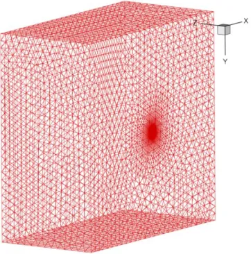
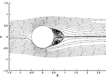
This case has been widely studied in literature, as documented by Johnson and Patel [60], and provides an initial qualitative assessment of the FVFLO-NCSU unstructured solver for a viscous flow. The test case presents a sphere within a laminar flow at a Mach number of 0.06 and Reynolds number of 100. At the prescribed flow conditions, a steady, axisymmetric flow exists, in which a toroidal vortex sits just aft of the sphere. Because the flow is axisymmetric, a hemisphere geometry is used with a symmetric boundary condition on the plane bisecting the sphere. The mesh for this case consists of 200416 tetrahedral elements and is shown in Fig. 5.4. Streamlines around the sphere computed by FVFLO-NCSU are shown in Fig. 5.5. The observed separation lies approximately 129 from the forward stagnation point, which agrees well with the results presented in [60].

Figure 5.5: Streamlines for laminar flow past a sphere computed by FVFLO-NCSU

This case was also used as a baseline for testing the parallel performance of the FVFLO-NCSU solver. The parallelization in FVFLO-NCSU follows the Single Program Multiple Data (SPMD) model, using the Message Passing Interface (MPI) standard. Partitioning of the computational domain is carried out using MeTiS [61]. Additional details on the parallelization of the FVFLO-NCSU solver may be found in [59]; further discussion in this paper is limited to simulation results.

Figure 5.6: Parallel speedup for the laminar sphere

Reacting Laminar Viscous Flow over a Flat Plate

Results are presented as both contour plots and line plots extracted along the gridlines

and . The Mach number distribution predicted by FVFLO-NCSU is in very good agreement with that generated by VULCAN, as seen in Fig. 5.7. However, the solutions for the temperature and H2O mass fractions, shown in Fig. 5.8, differ slightly between the two codes. The disagreements arise because these parameters are sensitive to the mixture thermal conductivity, and in this case the FVFLO-NCSU results were obtained using Wassiljewa’s formula, whereas the VULCAN results used an approach based on the assumption of a constant Prandtl number.

Figure 5.7: Mach number predictions for reacting laminar flow over a flat plate

Figure 5.8: Temperature (top group) and H2O mass fraction predictions

FVFLO Vulcan

Supersonic Turbulent Flow over a Flat Plate

To validate the implementation of the turbulence model within FVFLO-NCSU, a supersonic turbulent flow of non-reacting pre-mixed air (N2, O2, H2) over a flat plate was investigated. The flow has free stream temperature of 250 K, pressure of 25000 Pa, and velocity of 952 m/s, corresponding to a Reynolds number of over 20000000. Solutions are computed using three different grids. The first is a structured grid with 144 cells in both the and directions, for a total of 20736 hexahedral elements. The second is a hybrid grid, constructed by the hexahedral elements for in the original structured grid into two prismatic elements. The resulting grid consists of 14400 hexahedral and 12672 prismatic elements. The third is an unstructured grid consisting of 1232 prismatic elements and 5908 hexahedrals. The three grids are shown in Fig. 5.9.

Results for this case are presented as variable profiles in the direction at the exit of the domain ( ). The VULCAN solution on the structured grid is used as a baseline for comparing the FVFLO-NCSU solutions on each of the three grids. Fig. 5.10 shows that the -component velocity obtained by FVFLO-NCSU for all three grids are virtually identical to the VULCAN solution. The same is true of the temperature, seen in Fig. 5.11. Solutions for the turbulent variables and , shown in Figs. 5.12 and 5.13, also demonstrate good agreement with VULCAN; however, some discrepancies between the results generated by the two codes are evident, particularly near the surface of the plate. These differences in the turbulent variables can be attributed to slightly different approaches to implementation of the

Figure 5.10: Outlet profiles of -velocity for supersonic turbulent flat plate

Figure 5.12: Outlet profiles of turbulent kinetic energy for supersonic turbulent flat plate

Supersonic Turbulent Flow over a Flat Plate with Wall Matching

The turbulent flow over a flat plate was again simulated, this time to verify the wall matching procedure used in FVFLO-NCSU. The flow conditions and geometry used are identical to the previous flat plate problem. However, use of wall matching allows a significant reduction in the grid resolution required to obtain an accurate solution. So, while the computational mesh for this case is similar to the structured mesh of the previous case, it contains only 3600 hexahedral elements, with many fewer gridlines clustered around than for the solve-to-wall case. Solutions generated by FVFLO-NCSU are again compared to VULCAN results as flow variable profiles in the -direction at .

Figure 5.14: Outlet profiles of -velocity for wall matching flat plate

Figure 5.16: Outlet profiles of turbulent kinetic energy for wall matching flat plate

Supersonic Turbulent Reactive Flow over a Zero-Thickness Splitter Plate

This test case presents a zero-thickness splitter plate separating two incident flow streams. The first inflow stream, which enters the domain above the splitter plate, contains pure H2. The inflow stream that enters the domain below the splitter plate is an air mixture of species N2 and O2 with respective mass fractions of 0.7685 and 0.2315. Both inflow streams have a free stream static temperature of 1000 K and a free stream static pressure of atmosphere. The inflow velocity of the fuel stream is 3800 m/s, corresponding to a local Mach number of 1.6, while the air mixture inflow velocity is 1200 m/s, corresponding to a local Mach number of 1.9. The computational domain, shown in Fig. 5.18, consists of 41666 points and 20480 elements, and is included with the sample cases distributed with the VULCAN code.

Figure 5.18: Mesh for supersonic reacting splitter flow

Figure 5.19: Splitter plate temperature contours. FVFLO-NCSU (left); VULCAN(right)

The results shown in Figs. 5.19 and 5.20 demonstrate good agreement between the FVFLO-NCSU and VULCAN solutions. The H2O mass fraction profiles verify successful integration of VULCAN’s chemical reaction routines within FVFLO-NCSU; similarly the eddy viscosity ratio profiles verify the implementation of the Wilcox 1998 model within FVFLO-NCSU. Note that these solutions were generated using only first-order methods to eliminate any differences resulting from differences in second-order variable reconstruction between the unstructured and structured codes, to emphasize the successful use of the chemistry and turbulence routines within FVFLO-NCSU.

Turbulent Rectangular-to-Elliptical Shape Transition Scramjet Inlet

Figure 5.21: Configuration of modular REST inlets with actual computational domain in red

Figure 5.22: Computational mesh for REST inlet. Only one-quarter of grid points shown.

The REST inlet case was also used to further characterize the parallel performance of the FVFLO-NCSU solver. While the laminar sphere was run using up to 16 processes, the REST inlet simulations were carried out on up to 128 processes. Fig 5.25 compares the average wall time per iteration to number of processes used. The curve fit for the collected data is of the form ⁄ , indicating that the speedup is slightly less than ideal.

5.2 Hybrid VULCAN/FVFLO-NCSU Results

In this section, results generated by the integrated VULCAN/FVFLO-NCSU solver on hybrid meshes are presented. The developed unstructured patching procedure is compared to the original VULCAN structured patching method.

Reacting Inviscid Supersonic Flow into a 15 Compression Corner (II)

The first hybrid case presented is a simple test designed to demonstrate the basic integration of the FVFLO-NCSU code within VULCAN. In this case, the flow of an H2-Air mixture – comprised of 75.5% N2, 24% O2, and 0.5% H2 – at Mach 3.4 into a 15 compression corner is modeled. The free stream static temperature and pressure are 700 K and 1 atmosphere, respectively. At these flow conditions, an oblique shock wave attached to the wedge is formed, and a combustion reaction follows. The reaction model used for this case was again the NASA Langley 7 species and 7 reaction H2-Air kinetic model.

Figure 5.26: Hybrid mesh for supersonic compression corner

Inviscid Supersonic Flow over Two Bumps in a Channel

This test case presents an inviscid supersonic calorically perfect air flow over two consecutive bumps in a channel with a free stream Mach number of 2.0, a free stream static temperature of 256 K, and a free stream static pressure of 5637.5 Pa. This is very similar to a case that is included in the suite of sample cases distributed with VULCAN. The geometry for this test case consists of a channel containing two consecutive bumps along the lower surface.

Figure 5.28: Bumps in channel mesh for the patch-y (top) and hybrid-yz (bottom) cases

Figure 5.29: Unstructured patch for hybrid-y (left) and hybrid-yz (right) cases

Figure 5.32: Residuals for the two bumps in a channel test cases

Laminar Supersonic Flow over a Flat Plate

As with the patch-y bump case, the initial grid for the flat plate consists of two structured grids of differing resolution in the -direction separated patched together by a non-C0 interface. The grid for the patched flat plate case is shown in Fig. 5.33 along with the analogous hybrid grid, which has been superimposed below the original patched grid. The hybrid grid again contains a layer of hexahedral elements adjacent to the structured/unstructured interfaces, and prismatic elements are used to transition between the two blocks. A close up view of the unstructured block for the hybrid grid is shown in Fig. 5.34.

Figure 5.33: Grids for the flat plate patched and hybrid cases

Figure 5.36: Residual convergence for the patched and hybrid laminar flat plate

5.3 FVFLO-NCSU LES Results

Confined Supersonic Mixing Layer