Engineering Approach for Medium Modeling in Piping Dynamic Analysis

18th International Conference on Structural Mechanics in Reactor Technology (SMiRT 18) Beijing, China, August 7-12, 2005 SMiRT18-J01-2

ENGINEERING APPROACH FOR MEDIUM MODELING

IN PIPING DYNAMIC ANALYSIS

Peter S. Vasilyev

CKTI-Vibroseism Co. Ltd., St. Petersburg, Russian Federation

Phone: +7 812 3278599, Fax: +7 812 3278599

E-mail: [email protected]

ABSTRACT

Two approaches to the problem of dynamic interaction between pipe and medium are compared in the given paper: 1) The first one treats medium as mass rigidly connected to the pipe finite-element model’s nodes. 2) In the second one medium is modeled by the finite-element system of rod-elements. In this case the basic fluid-structure interaction (FSI) effects are taken into account.

The main techniques for FE modeling of some pipeline elements are presented in the paper. The second approach can be implemented by the use of general purpose FE programs. A model of a feed water pipeline of VVER-440 type NPP has been developed to study how the FSI affects on pipeline response. The results of the analysis which allow estimation of inaccuracy arising from medium dynamics neglecting are as follows:

- calculation of eigen frequency and mode shapes; - seismic analysis using the response-spectrum method;

- accidental blast impact assessment with the use of time history analysis; - operating vibration assessment on the basis of harmonic analysis.

It has become apparent that the way of medium modeling has an essential influence on the dynamic behavior of pipelines.

Keywords: fluid-structure interaction, pipe loads, vibration analysis, seismic analysis, pressure oscillation

1. INTRODUCTION

The medium mass is considered as non-structural mass (similar to thermal insulation mass) in most piping analyses which are carried out using the specific piping codes. The medium own dynamics therewith is ignored. From the other hand there is a set of problems which can not be solved without taking into account the medium dynamics factor. Among them are the following:

- water-hammer problem;

- whip movements of a pipe after its rupture; - flow-induced vibration of pipelines.

Two approaches may be applied when the medium dynamics problem can not be ignored:

- Uncoupled analysis that is performed in two steps. In the first step the hydrodynamic analysis is carried out with the assumption that a pipe is fixed and the interaction forces are calculated. Pipe oscillations caused by these forces are calculated in the second step.

- Coupled analysis in which hydrodynamic and mechanical tasks are supposed to be solved simultaneously. The solution of this task requires using the very specialized programs (Kratz, 2003). The latter approach known as Fluid-Structure Interaction is under active development nowadays.

In general FSI analysis is too complicated and expensive to be widely used.

A simplified method for FSI effects which allows carrying out such analyses using general purpose FE programs may be proposed for the limited set of tasks (Belytschko, 1986).

able to simulate medium column axial oscillations (along the pipeline axis). Medium mass should be rigidly connected to the steel part of a pipeline in transverse direction. This approach shall limit, of course, a set of tasks to be solved. These limitations will be discussed below.

The possibility of changing a hydrodynamic model with a linear elastic one can be based on the fact that small harmonic oscillations obey the general differential equation:

0

1

=

∂

∂

⋅

−

∂

∂

t

c

x

ξ

ξ

, (1)

where x is a spatial coordinate, t – time, c – sonic velocity, ξ - harmonic wave function. The wave function can represent the behavior of velocity, pressure, displacement, force etc.

There is a set of formulas for evaluating the applicability of the FSI analysis to the pipeline under consideration. Following the terms of Standard Review Plan 3.7.2 (US NRC, 1989), a pipeline as a whole can be considered as “seismic system” and medium inside the pipeline – as “seismic subsystem”. Two ratio - Rm and Rf –

can be calculated therewith. Rm is a ratio of the “seismic subsystem” mass to the mass of “seismic system”. Rf is a

ratio of fundamental frequency of the supported system to dominant frequency of the support motion. The following SPP criteria can be applied:

1) If Rm < 0.01, decoupling can be done for any Rf.

2) If 0.01 < Rm < 0.1, decoupling can be done only if Rf < 0.8 or Rf > 1.25.

3) If Rm > 0.1, a subsystem model should be included in the primary system model.

4) If “seismic subsystem” is rigid compared to “seismic system” and also is rigidly connected to it, such subsystem may be accounted by including the subsystem mass.

It is obvious that the latter point is used in conventional analysis of pipelines, however in this case the assertion of rigid medium seems to be questionable. Beside this the connection between pipe and medium is rigid just in transverse direction; there is no connection along pipe axis.

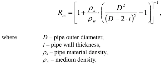
Rm ratio can be calculated for a pipeline as:

(

)

1

2

1





























−

⋅

−

⋅

+

=

t

D

D

R

_ρ

ρ

, (2)

where D – pipe outer diameter, t – pipe wall thickness,

ρs – pipe material density,

ρw – medium density.

Rm ratio calculation examples for some typical NPP pipes are given in Table 1.

Table 1. R

ratio calculation examples

Medium D, mm t, mm ρs, kg/m3 ρw, kg/m3 Rm

Water, p=9.0 Mpa 426 22 7800 1000 0.345

Water, p=0.29 Mpa 1220 10 7800 1000 0.792

Steam, p=6.8 Mpa 259 8 7800 33.5 0.0306

Steam, p=6.4 Mpa 426 24 7800 30.4 0.0142

As may be seen from the Table 1, the medium mass should be taken into account in case of water-filled pipelines, however it may be accounted just being added to the pipe mass provided that medium is rigidly connected to a pipe.

In case of steam-filled pipelines uncoupled analysis is permissible on condition that steam column eigen frequencies are spaced enough from dominant frequencies of the pipeline being excited.

For the simple pipes (without branches) the medium column eigen frequencies can be calculated by the following formulas:

,...

3

,

2

,

1

2

'

=

⋅

⋅

=

n

L

c

n

f

,...

5

,

3

,

1

4

'

=

⋅

⋅

=

n

L

c

n

f

where L – medium column height,

c’ – medium sonic velocity with consideration for pipe wall elasticity.

Formula (3) is applicable in calculations of pipes with two closed ends as well as of pipes with two open ends, but in the second case fundamental frequency is equal to zero. Formula (4) can be applied for the open-closed systems.

c’ value can be calculated by the Korteweg formula:

t

E

D

K

c

c

⋅

⋅

+

=

1

'

where c – medium sonic velocity,

Kw – bulk modulus of medium elasticity,

Es – Young’s modulus of elasticity of the pipe material.

Medium sonic velocity is calculated by:

w w

K

c

ρ

=

Water sonic velocity weakly depends on pressure and temperature and in most cases it is taken as constant value. Steam sonic velocity should be defined using specific tables and formulas. For low-compressible media such as water it is advisable to correct sonic velocity by the formula (5), that is of most importance for pipes with relatively thin walls. Examples of sonic velocity calculations for some typical pipelines are presented in Table 2. Acoustic pipe length (L20) calculated by formula (3) with f1 = 20 Hz is also given in this Table.

Table 2. Sonic velocity calculation examples

Medium p, MPa T, °C D, mm t, mm c, m/s Kw, MPa Es, MPa c’, m/s L20, m

Water 9.0 180 426 22 1460 2010 1.91*105 1331 33.3

Water 0.29 20 1220 10 1464 2140 2.00*105 964 24.1

Steam 6.8 285 259 8 503 8.48 1.82*105 503 12.6

Steam 6.4 297 426 24 523 8.32 1.81*105 523 13.1

Abovementioned data show that FSI can affect the calculation results even in cases of relatively short pipelines.

2. GENERAL ASSUMPTIONS

The following assumptions have been made:

- steady-state flow in a pipeline is ignored. The steady-state velocity value is supposed to be much lower then the sonic velocity and has no influence on medium oscillations;

with thin wall. Should this condition be met the beam model of a pipe remains correct and the medium mass can be connected to the beam node in transverse direction;

- Poisson coupling phenomenon is neglected;

- pipe-medium dynamic interaction occurs at such locations as bends, tees, reducers and closed ends where medium velocity or direction is changed;

- mutual friction coupling phenomenon is ignored;

- medium is considered to be homogenous. Multiphase media therewith can not be modeled;

- medium behavior is taken to be linear-elastic. Medium pressure oscillation is considered to be less than static pressure;

- thermodynamic effects due to pressure oscillation are ignored;

- dynamic displacements both of pipeline and medium are taken to be small in the FEM context, i.e. the task is still considered to be geometrically linear.

Damping at local hydraulic losses is not considered in this paper but can be easily implemented in the future. Thus, only the basic FSI effects and linear approach are taken into account in the proposed method.

3. MODELING TECHNIQUES

As it was mentioned above, coupled system analysis assumes the pipeline model consisting of two parts. The beam part of the model represents the steel structure oscillations. The rod part of the model represents the acoustic medium oscillations inside pipe. The beam model can be created in ordinary way – using the beam idealization, the medium mass therewith is ignored. Consideration for the bend flexibility factor is an important point of modeling. Should general purpose FE code be used this problem can be solved by decreasing bending moments of inertia for relevant elements. Bends should be meshed into several straight pipes to provide the required accuracy of calculations.

The rod model creation is discussed more detailed below.

3.1 Straight Pipes

Medium is modeled by the rod using nominal density, reduced Young’s modulus and cross section area calculated from the inner diameter. The reduced Young’s modulus is obtained from the rod sonic velocity as:

ρ

ρ

=>

=

⋅

=

)

'

(

'

E

E

c

c

The model detail in deformed state is shown in Fig.1.

Rod-element (green) has two own nodes, which are coincided in space with the correspondent nodes of beam-element (black). There are two additional nodes at each section, which spaced from central node toward local axes of the element.

The absolutely rigid element (red) has master node at a beam node and additional nodes as slave nodes. The node on a rod-element is connected to additional nodes by two spring-elements (blue), which have to be stiff enough. This combination of the elements provides free movement for rod-element along beam-element and no relative movements in transversal directions.

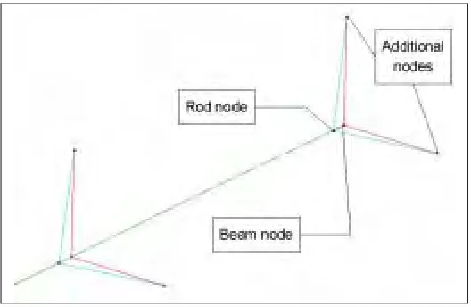
3.2 Bends

Bends are modeled similar to straight pipes. But we need to calculate free movement direction for each beam-element node. Two additional nodes have to be placed toward two orthogonal directions.

The model detail in deformed state is shown in Fig.2.

Fig. 2 Bend model

3.3 Reducers and Tees

The model for reducer is shown in fig. 3, and the model for tee is shown in fig. 4. Modeling is not so trivial these cases, because constant element volume condition has to be met. This condition can be expressed as:

∑

⋅

=

i i i

x

A

0

where Ai – adjacent pipe cross section area,

xi – nodal displacement toward the interior of reducer (tee).

In order to calculate geometry of the tee or reducer using formula (8) rod-elements have to be treated as rigid.

Fig. 3 Reducer model

Fig. 4 Tee model

3.4 Free ends

Free ends of the pipeline may be modeled as open end or as closed end. Medium velocity is equal to zero for the closed end. It may be cap, closed valve or pump. In order to model closed end a correspondent beam and rod nodes have to be merged. Closed valve inside pipeline can be modeled in the same way.

If the number of the open ends in the model is more than one, there will be several zero-frequency eigen modes. These eigen modes will correspond to free medium movement from one open end to the other. The same effect occurs if model has the closed loops.

It is usual conventional practice to limit the pipeline model at rigid support, wall penetration etc. Proposed approach requires including full acoustical length of the pipeline to the model. Generally the coupled FSI model will be longer than conventional.

4 SAMPLE MODEL

The main goal of this investigation is to estimate the order of inaccuracy, which arises from neglecting of FSI. This estimation can be done by comparison of the computational results obtained from two different models of the same pipeline.

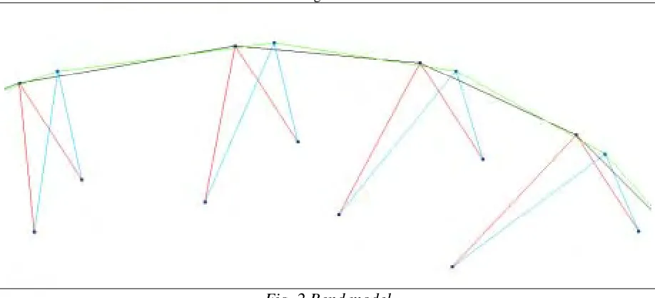
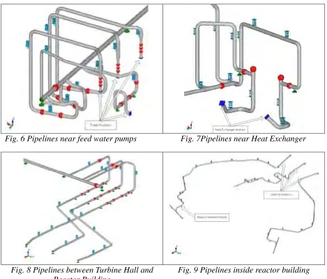
Feed water pipeline of the of VVER-440 type NPP was chosen to create these models. General model view is shown in Fig. 5. Some details are shown in Fig. 6, 7, 8 and 9.

Fig. 5 Sample model overview

The pipeline starts from the four pumps in the turbine hall and ends inside steam generators in the reactor building containment. Some simplifications were applied. The model includes approximately a half of the real feed water pipeline. Some auxiliary pipes were excluded. Steam generators treated to be rigid. Some model parameters are below:

Main dimensions (X x Y x Z): 71.5 x 52.1 x 24.7 m

Medium: Water

Pressure: 9.0 MPa

Temperature: 180 ‘C

Total length: 513 m

Pipe nomenclature (D x t): 426x22, 323x20, 273x15, 219x12 mm

Max. acoustic length: 214 m.

Estimated sonic velocity is 1331 m/s. The first estimated acoustic frequency is 3.1 Hz.

Model B was successfully verified against source (dPIPE) model. Some parameters for both models are compared in Table 3.

Fig. 6 Pipelines near feed water pumps

Fig. 7Pipelines near Heat Exchanger

Fig. 8 Pipelines between Turbine Hall and

Reactor Building

Fig. 9 Pipelines inside reactor building

Table 3. Parameters for the models

Parameter Model A Model B

Number of nodes 7557 2089

Number of elements 7574 2088

Number of DOFs 16461 10917

Overall mass, kg 154300 154350

Medium mass, kg (%) 35317 (22.9%) -

There are no closed loops in the model. All free ends in the Model A are treated as closed ends to avoid zero frequencies.

Equal damping is used for pipes and for medium in the samples discussed below. However real damping for medium is usually less than for piping. This case FSI effects may become higher.

5 EIGEN FREQUENCIES AND MODES

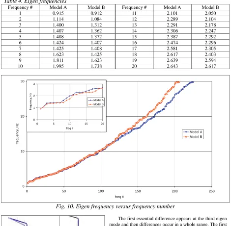
225 eigen frequencies were found in the range using Model A, and 206 frequencies - using Model B. Eigen frequencies versus frequency number are compared in Fig. 10.

Shown frequencies comparison allows to conclude that Model A frequencies in general are lower than Model B frequencies. Neverthless FSI effects can make eigen frequencies higher in the range below the first acoustic frequency.

Table 4. Eigen frequencies

Frequency # Model A Model B Frequency # Model A Model B

1 0.915 0.912 11 2.101 2.050

2 1.114 1.084 12 2.289 2.104

3 1.400 1.312 13 2.291 2.178

4 1.407 1.362 14 2.306 2.247

5 1.408 1.372 15 2.387 2.292

6 1.424 1.407 16 2.474 2.296

7 1.425 1.408 17 2.581 2.305

8 1.623 1.425 18 2.617 2.403

9 1.811 1.623 19 2.639 2.594

10 1.995 1.738 20 2.643 2.617

0 10 20 30

0 50 100 150 200 250

freq #

fr

eq

ue

nc

y,

H

z

Model A Model B

0 1 2 3

0 5 10 15 20

freq #

fr

eq

uency

, H

z

Model A Model B

Fig. 10. Eigen frequency versus frequency number

The first essential difference appears at the third eigen mode and then differences occur in a whole range. The first and the second eigen mode shapes are very similar for both models (see fig. 11 and 12).

Fig. 11 First eigen

mode (both models)

Fig. 12 Second

eigen mode

(both models)

The third eigen mode shape for the Model A is close to the forth eigen mode shape for the Model B. This mode is also located near the heat exchanger just as the first and the second ones. However in case of Model A rod-elements movement along beam-elements takes place, especially obvious near containment penetrations.

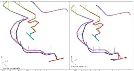
shapes are shown in fig. 13 and 14. Shapes are a bit different, but frequencies are essentially different.

Fig. 13 Model A. Eigen Mode #6

Fig. 14 Model B. Eigen mode #3

There are no purely acoustic eigen modes for the Model A. But medium (rod-element) movement occurs in most eigen modes. This result differs from steam pipeline analysis results (Vasilyev, 2003).

The first expected acoustic frequency for the Model A was equal 3.1 Hz. However FSI effects appear also in a lower frequency range.

6 SEISMIC ANALYSIS USING RESPONSE SPECTRUM ANALYSIS METHOD

Seismic analysis was made with SOLVIA code by applying RSA. Uniform damping was used. Response spectra are shown in Fig. 15. Eigen modes up to 30 Hz were taken into account. Missing mass effect correction was applied. Modal and spatial combinations were made by SRSS. No static analysis was applied.

Support reactions were selected to compare the results. There were selected only those dynamic reactions, which value was greater than 1000 N. Reactions in different directions were compared separately.

Fig. 15 Response Spectra

To quantify inaccuracy which arises from ignoring FSI, the value of relative difference (DR) is

used. DR is calculated by formula:

A B A R

R

R

R

D

=

−

where Ra - reaction value, obtained using Model A, Rb - reaction value, obtained using Model B.

Relative difference value will be negative if conventional analysis shows a greater reaction value, i.e. conventional analysis is conservative. Alternatively relative difference value will be positive. When DR runs up to

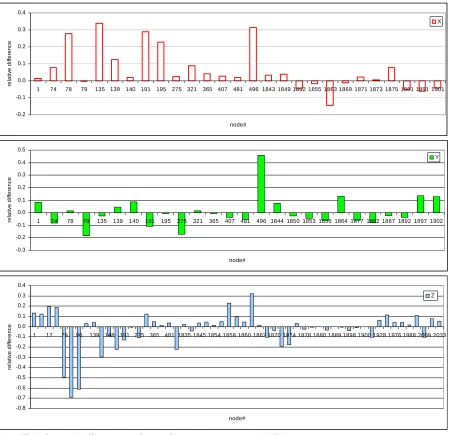
The relative difference values of support reaction calculations in directions X, Y and Z are given in Fig. 17.

-0.2 -0.1 0.0 0.1 0.2 0.3 0.4

1 74 78 79 135 139 140 191 195 275 321 365 407 481 496 1843 1849 1852 1855 1863 1869 1871 1873 1875 1881 1891 1901

node#

rel

at

iv

e di

ff

er

enc

e

X

-0.3 -0.2 -0.1 0.0 0.1 0.2 0.3 0.4 0.5

1 74 78 79 135 139 140 191 195 275 321 365 407 481 496 1844 1850 1853 1856 1864 1877 1882 1887 1892 1897 1902

node#

re

la

ti

v

e

dif

fer

enc

e

Y

-0.8 -0.7 -0.6 -0.5 -0.4 -0.3 -0.2 -0.1 0.0 0.1 0.2 0.3 0.4

1 12 79 90 139 148 191 275 365 481 1835 1845 1854 1858 1860 1862 1870 1874 1878 1880 1889 1898 1900 1928 1976 1988 2009 2033

node#

rel

at

iv

e

di

ff

er

enc

e

Z

Fig.17 Relative Difference values of support reactions (RSA)

Fig. 18 Max. D

locations (RSA)

non-conservative estimation. Relative difference maximum value is obtained for Y-reaction at the node# 496 (+45.9%). The location of the supports of the DR highest values is shown in Fig.18. In these figures callouts there

are numbers of nodes and relative difference values. Callouts colors correspond to the reaction directions (X – red, Y – green, Z – blue).

Contrary to Model B, Model A permit calculating dynamic pressure pulsations. In this analysis the dynamic pressure highest value has been registered in the pipeline branch adjacent to the node# 321 (see Fig.18). Its value runs up to 0.07 MPa (less then 1% of the static pressure). Though this value is not considered as hazardous in case of the given pipeline, this effect should be accounted in calculations of thin-walled pipelines operating under the low pressure.

7 ACCIDENTAL BLAST ANALYSIS USING TIME HISTORY ANALYSIS METHOD

Direct time-history analysis was carried out with SOLVIA code. Excitation originated from the external accidental blast is similar to the seismic excitation but lies in a higher frequency range. Reyleigh damping was used. No static loads were applied.

Similar to previous sample support reactions were selected to compare the results. There were selected only those dynamic reactions, which value was greater than 3000 N. Reactions in different directions were compared separately.

The relative difference values of support reaction calculations in directions X, Y and Z are given in Fig. 19.

-0.5 -0.4 -0.3 -0.2 -0.1 0 0.1 0.2 0.3 0.4 0.5 0.6

1 78 135 140 195 365 481 1843 1852 1863 1871 1875 1891

node# re la ti v e d iffe re n c e X -0.25 -0.2 -0.15 -0.1 -0.05 0 0.05

1 74 78 79 135 139 140 191 195 275 321 365 407 481 496 1844 1850 1853 1856 1864 1877 1882 1887 1892 1897 1902

node# re lat iv e dif fer enc e Y -0.6 -0.4 -0.2 0 0.2 0.4

79 140 321 496 1836 1851 1857 1859 1861 1865 1872 1876 1879 1888 1898 1928

node# re la ti v e d iffe re n c e Z

Fig.19 Relative Difference values of support reactions (THA)

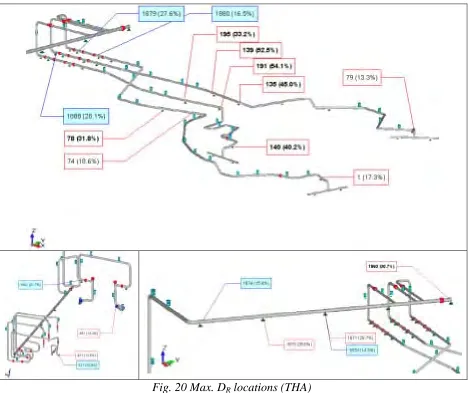
Fig. 20 Max. D

locations (THA)

In this analysis the dynamic pressure highest value has been registered in the pipeline branch adjacent to the steam generator nozzle. Its value runs up to 0.31 MPa (3.4% of the static pressure).

8 OPERATIONAL VIBRATION ASSESSMENT USING THE HARMONIC ANALYSIS

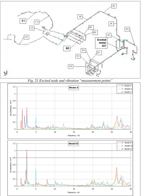
Operational vibration calculation has been carried out using the NE/NASTRAN code (Noran Eng., 2002) on the base of direct harmonic analysis. The construction damping has been set to 2%. Though the actual vibration often induces by flow (Olson, 2002), in our case excitation has been applied directly to the structure. The harmonic force of 300 N amplitude has been applied at the node# 227 (Fig.21) in X and Z directions. The excitation frequency was varied in the range from 1 to 30 Hz. The response accelerations were analyzed at nodes marked in Fig.21.

The response vibration acceleration spectra started to become different at the excited node (Fig.22).

Difference is getting more distinctive as one is moving away from the node excited. A typical example (for B3 point) is presented in Fig.23. Some peaks are very similar, others – not. Some peak values may differ by several times, however the overall vibration level (RMS) remains comparable for both models under consideration.

Fig. 21 Excited node and vibration “measurement points”

Model A

0 0.2 0.4 0.6 0.8 1 1.2

0 5 10 15 20 25 30

frequency, Hz

a

c

c

e

le

ra

ti

o

n

, m

/s

2

X - Model A

Y - Model A Z - Model A

Model B

0 0.2 0.4 0.6 0.8 1 1.2

0 5 10 15 20 25 30

frequency, Hz

a

c

c

e

le

ra

ti

o

n

, m

/s

2

X - Model B Y - Model B

Z - Model B

Model A 0 0.05 0.1 0.15 0.2 0.25 0.3

0 5 10 15 20 25 30

frequency, Hz ac c el erat ion, m /s 2

X - Model A Y - Model A Z - Model A

Model B 0 0.05 0.1 0.15 0.2 0.25 0.3

0 5 10 15 20 25 30

frequency, Hz ac c el er a ti on, m /s 2

X - Model B Y - Model B Z - Model B

Fig. 22 Vibration Spectra at point B3

Model A 0 0.05 0.1 0.15 0.2 0.25 0.3

0 5 10 15 20 25 30

frequency, Hz a cce le ra ti o n , m /s 2

X - Model A Y - Model A Z - Model A

Model B 0.E+00 1.E-08 2.E-08 3.E-08 4.E-08 5.E-08 6.E-08 7.E-08 8.E-08

0 5 10 15 20 25 30

frequency, Hz ac c el er a ti on, m /s 2

X - Model B Y - Model B Z - Model B

9 CONCLUSIONS

The method for accounting the basic mechanisms of FSI effects is proposed in this paper. This method allows carrying out the pipelines dynamic analysis with the use of general purpose FE programs.

It has been demonstrated that FSI has an essential influence on the pipeline dynamic behavior in a wide frequency range.

It has been shown that consideration of medium as the rigidly connected mass may lead to both conservative and non-conservative estimations of dynamic forces. Large differences have been demonstrated in estimating both system frequencies and support reactions.

The application of coupled FSI analysis is of special importance in modeling the actual systems operational vibration. Ignoring the medium modeling in this case will result in impossibility of creating calculation model which would properly reproduce the measurement results.

REFERENCES

Kratz, J., Munch, W., Ungar, K., (2003), The Influence of Fluid-structure Interaction on Pipe System Loads. SMiRT-17, J05-5.

Belytschko, T., Karabin M., Lin, J.I., (1986), "Fluid-Structure Interaction in Water-hammer Response of Flexible Piping", Journal of Pressure Vessel Technology, 108, p.249.

US NRC, (1989), Standard Review Plan 3.7.2. SEISMIC SYSTEM ANALYSIS. Rev. 2.

Berkovski, A., (1997), Computer Software Code for Piping Dynamic Analysis dPIPE, Verification Manual Report No. co06-96x.vvk-01.

SOLVIA Engineering AB, (2000), SOLVIA Verification Manual, Linear Examples.

Vasilyev, P., Fromzel L., (2003), Analytical Study of Piping Flow-Induced Vibration. Example of Implementation., SMiRT-17, J05-6.

Noran Egineering, Inc., (2002), NE/Nastran Verification Manual.