A Cartesian Cut‐Stencil Method for the Finite Difference Solution of PDEs in Complex Domains

(1)

Scholarship at UWindsor

Electronic Theses and Dissertations Theses, Dissertations, and Major Papers

2016

A Cartesian Cut

‐

Stencil Method for the Finite Difference Solution

A Cartesian Cut Stencil Method for the Finite Difference Solution

of PDEs in Complex Domains

Mohammadali Esmaeilzadeh

University of Windsor

Follow this and additional works at: https://scholar.uwindsor.ca/etd

Recommended Citation Recommended Citation

Esmaeilzadeh, Mohammadali, "A Cartesian Cut‐Stencil Method for the Finite Difference Solution of PDEs in Complex Domains" (2016). Electronic Theses and Dissertations. 5788.

https://scholar.uwindsor.ca/etd/5788

This online database contains the full-text of PhD dissertations and Masters’ theses of University of Windsor students from 1954 forward. These documents are made available for personal study and research purposes only, in accordance with the Canadian Copyright Act and the Creative Commons license—CC BY-NC-ND (Attribution, Non-Commercial, No Derivative Works). Under this license, works must always be attributed to the copyright holder (original author), cannot be used for any commercial purposes, and may not be altered. Any other use would require the permission of the copyright holder. Students may inquire about withdrawing their dissertation and/or thesis from this database. For additional inquiries, please contact the repository administrator via email

(2)

Difference Solution of PDEs in Complex Domains

By

Mohammadali Esmaeilzadeh

A Dissertation

Submitted to the Faculty of Graduate Studies

Through the Department of Mechanical, Automotive and Materials Engineering

in Partial Fulfillment of the Requirements for

the Degree of Doctor of Philosophy

at the University of Windsor

Windsor, Ontario, Canada

2016

(3)

A Cartesian Cut

‐

Stencil Method for the Finite

Difference Solution of PDEs in Complex Domain

by

Mohammadali Esmaeilzadeh

APPROVED BY:

H. Yang, External Examiner

Bombardier Aerospace, Montreal

M. Monfared

Department of Mathematics & Statistics

J. Defoe

Department of Mechanical, Automotive & Materials Engineering

O. Iqbal

Department of Mechanical, Automotive & Materials Engineering

N. Zamani

Department of Mechanical, Automotive & Materials Engineering

R. Barron, Co-Advisor

Department of Mechanical, Automotive & Materials

Engineering

R. Balachandar, Co-Advisor

Department of Mechanical, Automotive & Materials

Engineering

(4)

iii

AUTHOR’S DECLARATION of ORIGINALITY

I hereby certify that I am the sole author of this thesis and that no part of this thesis has been published or submitted for publication.

I certify that, to the best of my knowledge, my thesis does not infringe upon anyone’s copyright nor violate any proprietary rights and that any ideas, techniques, quotations, or any other material from the work of other people included in my thesis, published or otherwise, are fully acknowledged in accordance with the standard referencing practices. Furthermore, to the extent that I have included copyrighted material that surpasses the bounds of fair dealing within the meaning of the Canada Copyright Act, I certify that I have obtained a written permission from the copyright owner(s) to include such material(s) in my thesis and have included copies of such copyright clearances to my appendix.

(5)

iv ABSTRACT

A new finite difference formulation, referred to as the Cartesian cut-stencil finite difference method (FDM), for discretization of partial differential equations (PDEs) in any complex physical domain is proposed in this dissertation. The method employs unique localized 1-D quadratic transformation functions to map non-uniform (uncut or cut) physical stencils to a uniform computational stencil. The transformation functions are uniquely determined by the coordinates of the points on the physical stencil. In its basic formulation, 2nd-order central differencing is used to approximate derivatives in the transformed PDEs. The resulting finite difference equations can be solved by classical iterative methods.

In the case of a boundary node with a Dirichlet boundary condition, the prescribed value can be used directly in the calculations on the corresponding stencil adjacent to the boundary. However, for Neumann boundary nodes, discretization of the normal derivative in the Neumann condition is accomplished using one-sided approximations, producing an approximate value for the solution variable at the boundary. Then, the cut-stencil method allows stencils adjacent to boundaries to be treated in the same way as interior stencils, thus enabling finite difference calculations on arbitrarily complex domains.

This new formulation can be combined with the higher-order compact Padé-Hermitian method to produce higher-order cut-stencil schemes. Three different Cartesian cut-stencil formulations based on local 4th-order approximations are proposed and analyzed. It has been shown that global 4th-order accuracy can be achieved when the same order of accuracy is implemented at Neumann boundaries.

Comparison of numerical results for some manufactured problems with the exact solution verifies the capability of the cut-stencil method to deal with PDEs in regular and irregular shaped domains. Cartesian cut-stencil FDM solutions are also obtained for some classical engineering benchmark problems, including Prandtl’s stress function, steady or unsteady heat conduction and flow in a lid-driven cavity.

(6)

v DEDICATION

(7)

vi

ACKNOWLEDGEMENTS

I would first like to express my sincere thanks and deep sense of gratitude to my main supervisor and adviser Dr. Ronald Barron, for his expertise, knowledge, invaluable guidance and continuous support during the course of this research. He was always available and enthusiastic to discuss the topics of the research. I can remember times during the first steps of this research when he was available to meet twice a day. His deep knowledge, along with his patience and kindness, made this research possible. Like his former students, I would like to state that “I could not have imagined having a better advisor and mentor for my graduate study”. Dr. Barron, thank you for all your guidance, your help and your motivation, which supported and encouraged me to aim for this goal.

I also was very fortunate to work on my research with Dr. Ram Balachandar as my co-advisor. I am extremely grateful to him for his constant interest, invaluable support and knowledge during the course of my Ph.D. study at University of Windsor.

I would like to express my appreciation to my committee members for their time to review my research. Their comments and feedback have been appreciated.

I express my deepest thanks to all my friends and office mates for providing a friendly collegial environment in our research lab and for our group. I wish them all the best in all aspects of their life and endeavours.

I take the opportunity to thank all my relatives for their support and encouragement during my education. I particularly would like to express my acknowledgment to my uncle, Mohammadjafar, and his family for their excellent cooperation with my family and their patience, especially throughout my father’s terminal illness.

(8)

vii

TABLE of CONTENTS

AUTHOR’S DECLARATION of ORIGINALITY ... iii

ABSTRACT ... iv

DEDICATION ... v

ACKNOWLEDGEMENTS ... vi

LIST of TABLES ... xii

LIST of FIGURES ... xvi

NOMENCLATURE ... xxiii

LIST of ABBREVIATIONS ... xxv

CHAPTER 1: INTRODUCTION to PARTIAL DIFFERENTIAL EQUATIONS and NUMERICAL METHODS... 1

1.1 Objective of the Chapter ... 1

1.2 Partial Differential Equations ... 1

1.3 Finite Difference Method: Basic Definitions, Strengths, Limitations ... 2

1.3.1 Discretization of Derivatives in FDM ... 3

1.3.2 Iterative Solution Algorithms ... 4

1.3.3 Ghost Node Method for Neumann Boundary Condition Treatment in TFDM ... 5

1.4 Transformation of PDEs ... 7

1.5 Cartesian Grid ... 8

1.6 Finite Volume Method: Basic Definition and Fundamentals... 9

1.7 Thesis Layout ... 11

CHAPTER 2: FUNDAMENTALS and FORMULATIONS of CARTESIAN CUT-STENCIL FINITE DIFFERENCE METHOD ... 12

2.2 Model Equation and General Transformation Functions ... 12

2.3 Arbitrary Domains and Cartesian Grid ... 13

2.4 Quadratic Form of the Transformation Functions ... 13

2.4.1 Mapping of an Arbitrary 5-point Stencil ... 14

2.4.2 Transformation and Discretization of the Model Convection-Diffusion Equation ... 15

2.5 Treatment of Boundary Nodes and Conditions ... 16

2.5.1 Implementation for Curved Boundaries with Neumann Condition ... 20

2.5.2 Treatment of Regular Boundary Nodes ... 21

(9)

viii

2.6 Higher-Order Differencing ... 29

2.6.1 5+4-point (4 Auxiliary Nodes) Stencil Formulation ... 30

2.6.1.1 Evaluation of Metrics at Auxiliary Nodes of 5+4-point Stencil Formulation ... 32

2.6.1.2 Evaluation of the Governing Function at Auxiliary Nodes in the 5+4-point Stencil Formulation ... 35

2.6.2 Higher-Order (HO) Padé-Hermitian Compact Cut-Stencil FD Formulation ... 36

2.6.2.1 Approximation of First Derivatives in Compact Padé-Hermitian Finite Differencing ... 37

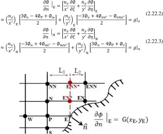
2.6.2.2 Approximation of Second Derivatives in Compact Padé-Hermitian Finite Differencing . 38 2.6.3 Comparison of the Stencil of Higher-Order Compact (Implicit) and Explicit Finite Difference Methods ... 39

2.6.4 Higher-Order Cut-Stencil Finite Difference Method (HO Cut-Stencil FDM) for Convection-Diffusion Equation ... 40

2.6.5 Higher-Order Cut-Stencil Finite Difference Method for Boundaries Nodes ... 47

2.7 Cut-Stencil FD Formulation of Unsteady Model Equation ... 49

2.7.1 Explicit Forward in Time and Central in Space (FTCS) Formulation of the Cut-Stencil FDM ... 50

2.7.1.1 Stability Analysis for FTCS Formulation of Cut-Stencil FDM ... 51

2.7.2 Cut-Stencil FDM Formulation for Second-Order Wave Equation ... 53

2.7.2.1 1st -Order Accurate Approximation for First Temporal Derivative at Initial Time for Second-Order Wave Equation ... 54

2.7.2.2 2nd -Order Accurate Approximation for First Temporal Derivative at Initial Time for Second-Order Wave Equation ... 55

2.7.2.3 Stability Analysis for Cut-Stencil Formulation of Second-Order Wave Equation ... 56

2.8 Chapter Summary ... 56

CHAPTER 3: CARTESIAN CUT-STENCIL FDM SOLUTIONS to MANUFACTURED PROBLEMS ... 58

3.2 Definition of Method (Code) Verification ... 58

3.2.1 Method of Manufactured Solutions (MMS) ... 58

3.3 Local Truncation Error (LTE) ... 59

3.3.1 Temporal Local Truncation Error for FTCS Formulation ... 62

3.3.2 Procedure for Calculation of Spatial Local Truncation Error (LTE) ... 63

3.4 Verification of Formal Accuracy of the Numerical Scheme ... 64

(10)

ix

3.5.1 Problem 1: Solution of Poisson Equation on a Square Domain with Dirichlet Boundary

Conditions Using the 2nd-Order 5-point Cut-Stencil Formulation ... 65

3.5.2 Problem 2: Solution of Poisson Equation on a Square Domain a with Neumann Boundary Condition Using the 2nd-Order 5-point Cut-Stencil Formulation ... 66

3.5.3 Problem 3: Solution of Poisson Equation on a Square Domain with Combination of Neumann Conditions on More Than One Boundary Using 2nd-Order 5-point Cut-Stencil Formulation ... 69

3.5.4 Problem 4: Solution of Convection-Diffusion Equation on Rectangular Domain Using 2nd -Order 5-point Cut-Stencil Formulation ... 71

3.5.5 Problem 5: 2nd-Order 5-point Cut-Stencil FD Solution of Laplace Equation on an Arbitrary, Irregular Shaped Domain ... 76

3.5.6 Problem 6: 2nd-Order 5-point Cut-Stencil FD Solution of Convection-Diffusion Equation on an Arbitrary, Irregular Shaped Domain ... 78

3.5.7 Problem 7: Comparison of 5-point 2nd-Order and 5+4-point Stencil Formulations of Cut-Stencil FDM to Solution of Poisson Equation in a Rectangular Domain ... 80

3.5.8 Problem 8: HO Cut-Stencil FDM1 Solution of PDEs in Rectangular and Irregular Shaped Domains ... 83

3.5.9 Problem 9: HO Cut-Stencil FDM2 Solution of PDEs in Rectangular and Irregular Shaped Domains ... 87

3.5.10 Problem 10: Cartesian Cut-Stencil FDM Solutions for Unsteady PDEs on Rectangular and Irregular Shaped Domains ... 93

3.5.11 Problem 11: Cut-Stencil FDM Solution for Second-Order Wave Equation on Rectangular and Irregular Shaped Domains ... 97

CHAPTER 4: CARTESIAN CUT-STENCIL FDM SOLUTIONS to SOLID MECHANICS and HEAT TRANSFER PROBLEMS ... 102

4.2 Application of Cut-Stencil FDM in Elasticity ... 102

4.2.1 Stress Function of Torsion for Straight Bars ... 102

4.2.2 Stress Function for Bending of Bars ... 106

4.3 Application of Cut-Stencil FDM to Heat Transfer Problems on Regular and Irregular Shaped Domains ... 108

4.3.1 Steady Conduction Heat Transfer in a Rectangular Domain ... 108

4.3.2 Steady Conduction Heat Transfer in an Irregular Domain ... 112

4.3.3 Unsteady Heat Conduction in a Rectangular Domain ... 114

4.3.4 Unsteady Heat Conduction in an Irregular Domain ... 116

(11)

x

CHAPTER 5: CUT-STENCIL FD FORMULATION for the SOLUTION of LID-DRIVEN

CAVITY FLOW ... 119

5.2 Primitive Variable Formulation of the Navier-Stokes Equations ... 119

5.3 Streamfunction-Vorticity Equations ... 120

5.4 Mapped Form of Streamfunction-Vorticity Equations and Boundary Conditions for Lid-Driven Cavity Flow ... 120

5.4.1 2nd-Order Discretization of Streamfunction-Vorticity Equations ... 122

5.4.2 Higher-Order (HO) Discretization of Streamfunction-Vorticity Equations... 123

5.4.2.1 Higher-Order Cut-Stencil Finite Differencing Method 1 (HO Cut-Stencil FDM1) for Streamfunction-Vorticity Equations ... 123

5.4.2.2 Higher-Order Cut-Stencil Finite Differencing Method 2 (HO Cut-Stencil FDM2) for Streamfunction-Vorticity Equations ... 124

5.4.3 Vorticity Boundary Condition Approximation ... 125

5.5 Numerical Results of Cut-Stencil FDM for Square Lid-Driven Cavity Flow ... 128

5.5.1 Numerical Results for 2nd-Order Discretization of Streamfunction-Vorticity Equations 129 5.5.1.1 𝑅𝑒 = 100 with Non-Uniform 129*129 Grid; Boundary Vorticity Approximated by Briley’s Formula ... 129

5.5.1.2 𝑅𝑒 = 1000 with Non-Uniform 129*129 Grid; Boundary Vorticity Approximated by Briley’s Formula ... 131

5.5.1.3 𝑅𝑒 = 100 and 𝑅𝑒 = 1000 with Non-Uniform 129*129 Grid; Boundary Vorticity Approximated by Compact Method ... 135

5.5.2 Higher-Order Cut-Stencil FD Solution to Lid-Driven Flow in a Square Cavity ... 136

5.5.2.1 Results of Higher-Order Discretization (𝑅𝑒 = 100) ... 136

5.5.2.2 Results for 2nd -Order and Higher-Order Discretizations (𝑅𝑒 = 400) ... 141

5.5.2.3 Results of Higher-Order Discretization (𝑅𝑒 = 1000) ... 149

5.6 Cut-Stencil FDM Solution of Lid-Driven Cavity Flow in Irregular Shaped Domains .... 158

5.6.1 Cut-Stencil FD Solution for the Lid-Driven Skewed Cavity Flow ... 158

5.6.2 Cut-Stencil FD Solution for Lid-Driven Right-Side and Left-Side Aligned Right Triangular Cavity Flow ... 168

5.6.3 Cut-Stencil FD Solution for Lid-Driven L-Shaped Cavity Flow ... 174

CHAPTER 6: CONCLUDING REMARKS and RECOMMENDATIONS for FUTURE WORKS ... 178

(12)

xi

6.2 Recommendations for Future Work ... 179

REFERENCES ... 181

APPENDIX I: SUMMARY OF MANUFACTURED PROBLEMS ... 193

APPENDIX II: DERIVATION of 2nd-ORDER ACCURATE APPROXIMATION for VORTICITY on a STRAIGHT WALL ... 194

A.II.1 Derivation of Briley’s Formulation ... 194

A.II.2 Derivation of a Compact 2nd-Order Formulation ... 195 APPENDIX III: CLUSTERING FUNCTION for NON-UNIFORM GRID GENERATION for LID-DRIVEN CAVITY FLOW in SQUARE DOMAIN ... 197

APPENDIX IV: VORTICITY EVALUATION on SLOPED or CURVED WALLS ... 199

(13)

xii

LIST of TABLES

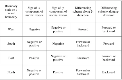
Table 2.1: Summary of the sign of normal vector components and corresponding differencing schemes for boundary nodes on curved boundaries ... 25

Table 2.2: Expressions for x- and y-coordinates of four auxiliary nodes on the physical stencil used in the 5+4-point cut-stencil formulation ... 31

Table 2.3: Metrics at four auxiliary nodes in 5+4-point stencil formulation ... 34 Table 2.4: Taylor’s series expansion used to derive the first derivative approximation in HOC finite difference method ... 37

Table 2.5: Taylor’s series expansion used to derive the second derivative approximation in HOC finite difference method ... 38

Table 3.1: Relative error, LTE and RMS results for Problem 1 ... 66

Table 3.2: Relative error and LTE results for Problem 2 (west Neumann boundary condition) ... 67

Table 3.3: Relative error and LTE results for Problem 2 (north Neumann boundary condition) .. 68

Table 3.4: Relative error and LTE results for Problem 3 (west & east Neumann boundary conditions) ... 69

Table 3.5: Relative error and LTE results for Problem 3 (west & south Neumann boundary conditions) ... 70

Table 3.6: Relative error and LTE results for Problem 4 with Dirichlet boundary conditions ( ν = 1,𝑃 = 𝑄 = 0.02, α = β = 0 ) ... 72

Table 3.7: Relative error and LTE results for Problem 4 with east and north Neumann boundary conditions (ν = 1, 𝑃 = 𝑄 = 0.02, α = β = 0) ... 73

Table 3.8: Relative error and LTE results for Problem 4 with Dirichlet boundary conditions (ν = 1, 𝑃 = 𝑄 = 0.02, α = β = −1) ... 74

Table 3.9: Relative error and LTE results for Problem 4 with Dirichlet boundary conditions (ν = 0.08, 𝑃 = 𝑄 = 1, α = β = 0, −1) ... 75

Table 3.10: Relative error, RMS error and maximum LTE for Problem 5 (Laplace equation, Dirichlet boundary conditions) ... 77

Table 3.11: Relative error, RMS error and maximum LTE for Problem 5 (Laplace equation, Neumann boundary conditions) ... 77

Table 3.12: Relative error results for Problem 6 (convection-diffusion equation) ... 79

Table 3.13: Comparison of results for 2nd-order 5-point stencil and 5+4-point cut-stencil formulations for Problem 6 (Dirichlet boundary condition) ... 81

(14)

xiii

Table 3.15: HO cut-stencil FDM1 solution to Problem 8.1 (Poisson equation, Dirichlet boundary conditions) ... 83

Table 3.16: Comparison of results for 2nd-order 5-point stencil and HO-FDM1 5-point stencil formulations for Problem 8.2 (diffusion equation) ... 85

Table 3.17: Comparison of results for 2nd-order 5-point stencil and the HO cut-stencil FDM1 for Problem 8.3 (convection-diffusion equation) ... 86

Table 3.18: Comparison of results for 2nd-order 5-point stencil and HO-FDM2 5-point stencil formulations for Problem 9 (diffusion equation) ... 88

Table 3.19: Errors from HO cut-stencil FDM2 solution for Problem 9.2 on irregular domain – (diffusion equation, Dirichlet boundary conditions) ... 89

Table 3.20: Comparison of results for 2nd-order 5-point stencil, HO-FDM1 5-point stencil and HO-FDM2 5-point stencil formulations for Problem 9.3 (convection-diffusion equation) ... 90

Table 3.21: Comparison of results of different schemes for Problem 9.4 (diffusion equation, different orders used for Neumann boundaries) ... 92

Table 3.22: Comparison of relative error, spatial and temporal truncation error and RMS error at

𝑡 = 1.76 for Problem 10.1 (unsteady diffusion) ... 95

Table 3.23: Average and relative errors and LTEs at different time with Δ𝑡 = 0.0625 for Problem 10.2 (unsteady diffusion, irregular domain) ... 97

Table 3.24: Comparison of relative and RMS errors at 𝑡 = 1.326 for Problem 11.1 (second-order wave equation) ... 99

Table 3.25: Comparison of relative error at t = 1.42 for Problem 11.2 (wave equation, irregular shaped domain ... 100

Table 4.1: Relative error for cut-stencil solution to Prandtl’s stress function for torsion of a bar with elliptical cross-section ... 105

Table 4.2: Absolute error for cut-stencil solution of Prandtl’s stress function for bending of a bar with elliptical cross-section beam ... 108

Table 4.3: Numerical and analytical solution for 2-D steady conduction heat transfer in rectangular plate ... 111

Table 4.4: Comparison of cut-stencil FDM and FVM for solution of steady conduction heat transfer in an irregular domain ... 113

Table 4.5: Comparison of cut-stencil FDM and TFDM for solution of unsteady conduction heat transfer in a rectangular domain ... 115

Table 4.6: Comparison of cut-stencil FDM and TFDM steady-state solution of the transient conduction heat transfer with analytical solution ... 116

Table 4.7: Comparison of cut-stencil FDM and FVM for solution of unsteady conduction heat transfer in an irregular domain at 𝑡 = 2 (s) ... 117

(15)

xiv

Table 5.2: Independency of solution to relaxation factor 𝜎 for 2nd-order accurate solution (𝑅𝑒 =

1000, non-uniform 129*129 grid) ... 132

Table 5.3: Comparison of 2nd-order accurate cut-stencil solution for lid-driven cavity flow (𝑅𝑒 = 1000, non-uniform 129*129 grid) ... 133

Table 5.4: Comparisons of 2nd-order accurate cut-stencil solution to lid-driven cavity flow using compact method for vorticity approximation on boundaries to results of Ghia et al. [150] (𝑅𝑒 =

100, 1000) ... 135

Table 5.5: Comparison of higher-order cut-stencil solutions for lid-driven cavity flow (𝑅𝑒 = 100, non-uniform 41*41 grid) ... 137

Table 5.6: 2nd-order and higher-order cut-stencil solutions for lid-driven cavity flow (𝑅𝑒 = 100, different non-uniform grid sizes) ... 138

Table 5.7: 2nd-order cut-stencil solutions and comparison to literature for lid-driven cavity flow (𝑅𝑒 = 400, different non-uniform grids) ... 141

Table 5.8: HO-FDM1 solution to lid-driven cavity flow on a square using higher-order compact upwind scheme for approximation of convective terms (𝑅𝑒 = 400, non-uniform 65*65 grid) .. 143

Table 5.9: Independency of solution to relaxation factor 𝜎 for HO-FDM1 (𝑅𝑒 = 400, non-uniform 65*65 grid) ... 144

Table 5.10: Solution for HO-FDM1 formulation to lid-driven cavity flow on a square using higher-order compact upwind scheme for approximation of convective terms (𝑅𝑒 = 400, non-uniform 81*81 grid) ... 145

Table 5.11: Higher-order cut-stencil FD solutions for lid-driven cavity flow (𝑅𝑒 = 400, different non-uniform grids) ... 145

Table 5.12: Comparison of velocity components at midpoint of domain and vorticity at midpoint of moving wall for HO cut-stencil FD solutions with Ghia et al. [150] (𝑅𝑒 = 400) ... 146

Table 5.13: Solutions of HO cut-stencil formulations for lid-driven cavity flow on a square using higher-order compact upwind scheme for approximation of convective terms (𝑅𝑒 = 1000, non-uniform grid) ... 149

Table 5.14: Independency of solution to relaxation factor 𝜎 for HO-FDM1 solution (𝑅𝑒 = 1000, non-uniform 65*65 grid) ... 150

(16)

xv

Table 5.19: Comparison of velocity components at midpoint of the domain and vorticity at midpoint of the moving wall for HO cut-stencil FD solutions with Ghia et al. [150] (𝑅𝑒 = 1000) . ... 154

Table 5.20: Comparison of 2nd-order accurate cut-stencil solution to other studies for lid-driven cavity flow (𝑅𝑒 = 1000, non-uniform 101*101 grid) ... 157

Table 5.21: Comparison of vorticity and velocity components at midpoint of domain and vorticity at midpoint of moving wall (𝑅𝑒 = 1000) ... 158

Table 5.22: Comparison of cut-stencil FD solutions to literature for skewed lid-driven cavity flow (𝑅𝑒 = 100, 𝛼 = 45˚) ... 160

Table 5.23: Cut-stencil FD solutions to skewed lid-driven cavity flow using upwind schemes (𝑅𝑒 = 1000, 𝛼 = 45˚, 4617 active nodes) ... 161

Table 5.24: Independency of skewed cavity solution to relaxation factor 𝜎 for 2nd-order cut-stencil formulation (𝑅𝑒 = 1000, 𝛼 = 45˚, 18193 active nodes)... 161

Table 5.25: Comparison of cut-stencil FD solutions for skewed lid-driven cavity flow (𝑅𝑒 =

1000, 𝛼 = 45˚) ... 162

Table 5.26: Comparison of cut-stencil FD solutions to Erturk and Dursun [187] for skewed lid-driven cavity flow (𝑅𝑒 = 100, 𝛼 = 135˚) ... 164

Table 5.27: Cut-stencil FD solutions for skewed lid-driven cavity flow using upwind schemes for approximation of convective terms for (𝑅𝑒 = 1000, 𝛼 = 135˚, 4617 active nodes) ... 165

Table 5.28: Independency of skewed cavity solution to relaxation factor 𝜎 for cut-stencil HO-FDM1 formulation (𝑅𝑒 = 1000, 𝛼 = 135˚, 18193 active nodes) ... 165

Table 5.29: Comparison of cut-stencil FD solutions with Erturk and Dursun [187] for skewed lid-driven cavity flow (𝑅𝑒 = 1000, 𝛼 = 135˚) ... 166

Table 5.30: Comparison of cut-stencil FD solutions for lid-driven cavity flow in a left-side aligned right triangle (𝑅𝑒 = 500) ... 169

Table 5.31: Comparison of cut-stencil FD solutions for lid-driven cavity flow in a left-side aligned right triangle (𝑅𝑒 = 1000) ... 170

Table 5.32: Comparison of cut-stencil FD solutions for lid-driven cavity flow in a right-side aligned right triangle (𝑅𝑒 = 500) ... 172

Table 5.33: Comparison of cut-stencil FD solutions to literature for lid-driven cavity flow in a right-side aligned right triangle at 𝑅𝑒 = 1000 ... 173

Table 5.34: Comparison of cut-stencil FD solutions for lid-driven cavity flow in an L-shaped domain (𝑅𝑒 = 1000) ... 175

Table A.I.1: Summary of manufactured problems studied in Chapter 3 ... 193 Table A.II.1: Taylor’s series expansions used to derive Briley’s equation to approximate the wall vorticity ... 194 Table A.II.2: Taylor’s series expansions used to derive the 2nd

(17)

xvi

LIST of FIGURES

Figure 1.1: Uniform grid system used for solution of Poisson equation ... 4

Figure 1.2: Schematic of grid system showing ghost node for approximation of imposed Neumann condition on the lower boundary ... 6

Figure 1.3: Sample of a 2-D grid transformation, a) physical domain, and b) computational domain... 7

Figure 1.4: Schematic of Cartesian grid system for an arbitrary body ... 9

Figure 1.5: Schematic of control volume used for FVM solution to Laplace equation ... 10

Figure 2.1: Arbitrary complex domain with Cartesian grid and cut-stencils ... 13

Figure 2.2: Mapping from an arbitrary physical stencil to a generic computational stencil in 2-D ... 14

Figure 2.3: Mapping of (a) uncut physical stencil, and (b) cut physical stencil, to a uniform computational stencil ... 15

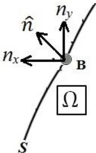
Figure 2.4: Boundary curve and normal vector at specific point ... 17

Figure 2.5: Uniform Cartesian grid used for one-sided differencing of Neumann boundary condition (TFD notation) ... 17

Figure 2.6: Sample grid used for one-sided differencing of Neumann boundary condition (cut-stencil FD notation) ... 18

Figure 2.7: Illustration of two five-point stencils in neighbouring a) physical stencils, b) generic computational stencils ... 19

Figure 2.8: Sample of five-point stencil with Neumann conditions at two endpoints ... 20

Figure 2.9: Illustration of regular and irregular boundary nodes ... 21

Figure 2.10: Regular boundary node at west node of physical stencil with 𝑛_𝑦< 0 ... 22

Figure 2.11: Regular node at west boundary node of physical stencil with 𝑛𝑦> 0 ... 23

Figure 2.12: Regular node at south boundary node of physical stencil with 𝑛𝑥 < 0 ... 23

Figure 2.13: Regular node at south boundary node of physical stencil with 𝑛_𝑥> 0 ... 24

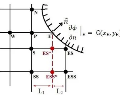
Figure 2.14: Irregular node at east boundary node of physical stencil with 𝑛_𝑦> 0 ... 26

Figure 2.15: Irregular node at east boundary node of physical stencil with 𝑛𝑦< 0 ... 27

Figure 2.16: Irregular node at north boundary node of physical stencil with 𝑛𝑥 < 0 ... 27

Figure 2.17: Illustration of a regular boundary node with Neumann condition at the endpoints of two 5-point stencils ... 28

(18)

xvii

Figure 2.20: 5+4-point main stencil along with four 5-point stencils at the auxiliary nodes, a) physical illustration, b) computational illustration ... 33

Figure 2.21: Mapping from point physical stencil located at auxiliary node L to a uniform 5-point computational stencil centred at auxiliary node l ... 33

Figure 2.22: Mapping from point physical stencil located at auxiliary node B to a uniform 5-point computational stencil centred at auxiliary node b ... 34

Figure 2.23: Cut-stencils not directly applicable to the 5+4-point cut-stencil formulation, a) intersection with straight oblique boundary line, b) intersection with curved boundary line .... 36

Figure 2.24: Comparison of the stencil for 4th-order accurate approximations, a) compact FD (implicit) scheme, b) explicit FD scheme ... 39

Figure 2.25: Computational stencil for central or one-sided second-order approximations of derivatives at the endpoints of a stencil used in HO-FDM1 ... 43

Figure 2.26: Computational stencil for central or one-sided first-order approximations of second derivatives at the endpoints of a stencil used in HO-FDM1 ... 44

Figure 2.27: Computational stencil for central or upwind 4th-order approximations of first derivatives at the endpoints of a stencil used in HO-FDM2 ... 45

Figure 2.28: Computational stencil for 3rd-order approximations of first derivatives at the endpoints of a stencil used in HO-FDM2 ... 46

Figure 2.29: Schematic used for higher-order differencing at a boundary node with Neumann condition in TFD notation (in 𝑥 direction) ... 48

Figure 2.30: Schematic used for higher-order differencing at boundary node with Neumann condition in TFD notation (in 𝑦 direction) ... 48

Figure 2.31: Computational stencil for higher-order differencing at boundary nodes with Neumann condition (cut-stencil FD notation) ... 49

Figure 2.32: Illustration of stencil used for explicit FTCS formulation... 50

Figure 3.1: Verification plot for global order of accuracy for Problem 1 ... 66

Figure 3.2: Verification plot for global order of accuracy for Problem 2 (west Neumann condition) ... 67

Figure 3.3: Verification plot for global order of accuracy for Problem 2 (north Neumann condition) ... 68

Figure 3.4: Verification plot for global order of accuracy for Problem 3 (west and east Neumann condition) ... 70

Figure 3.5: Verification plot for global order of accuracy for Problem 3 (west and south Neumann condition) ... 71

Figure 3.6: Variation of maximum relative error of internal and boundary nodes for different cell sizes (combination of Neumann boundary conditions) ... 71

(19)

xviii

Figure 3.8: Verification plot for global order of accuracy for Problem 4, Neumann boundary conditions on east and north (ν = 1, 𝑃 = 𝑄 = 0.02, α = β = 0) ... 74

Figure 3.9: Verification plot for global order of accuracy for Problem 4, Dirichlet boundaries (ν = 1, 𝑃 = 𝑄 = 0.02, α = β = −1) ... 75

Figure 3.10: Verification plot for global order of accuracy for Problem 4, Dirichlet boundaries (ν = 0.08, 𝑃 = 𝑄 = 1, α = β = −1) ... 76

Figure 3.11: Irregular shaped domain used for Problem 5 ... 77

Figure 3.12: Verification of global order of accuracy for Problem 5 (Laplace equation) ... 78

Figure 3.13: Irregular shaped domain with non-uniform grid and cut-stencils for Problem 5 (convection-diffusion equation) ... 79

Figure 3.14: Ratio of maximum absolute error of 2nd-order 5-point stencil to 5+4-point stencil methods vs. 𝒽 for Problem 7 (Dirichlet boundary conditions) ... 81

Figure 3.15: Verification plot for global order of accuracy for Problem 7 (west and east Neumann boundary condition) ... 82

Figure 3.16: Comparison of absolute errors along centrelines of domain of Problem 7 (Neumann conditions on west and east boundaries), (a,b) 153 nodes, (c,d) 2145 nodes ... 83

Figure 3.17: Verification plot for global order of accuracy for Problem 8.1 and comparison with Problem 7 (Dirichlet boundary conditions) ... 84

Figure 3.18: Irregular domain illustration for Problem 8.2 (diffusion equation) ... 85

Figure 3.19: Irregular shaped domain for Problem 8.3 (convection-diffusion equation) ... 86

Figure 3.20: Verification plot for global order of accuracy for Problem 9.1 (diffusion equation, Dirichlet boundary conditions) ... 88

Figure 3.21: Verification plot for global order of accuracy for Problem 9.2 (diffusion equation on irregular domain, Dirichlet boundary conditions) ... 89

Figure 3.22: Irregular shaped domain for Problem 9.3 (diffusion-convection equation) ... 90

Figure 3.23: Verification plot for global order of accuracy for Problem 9.4 (diffusion equation, Neumann boundary conditions) ... 93

Figure 3.24: Exact solution 𝜙(𝑥, 𝑦, 5) for Problem 10.1 (unsteady diffusion) ... 94

Figure 3.25: Cut-stencil FDM solution at 𝑡 = 5.0 for grid of 121 nodes for Problem 10.1, a) Δ𝑡 = 0.04 , b) Δ𝑡 = 0.05 (unsteady diffusion) ... 94

Figure 3.26: Verification plot for global order of accuracy for spatial discretization for Problem 10.1 (unsteady diffusion) ... 95

Figure 3.27: Irregular shaped domain for Problem 10.2 (unsteady diffusion) ... 96

(20)

xix

Figure 3.29: Exact and cut-stencil FDM solutions at 𝑡 = 0.84 for grid of 441 nodes for Problem 11.1, a) exact solution, b) Δ𝑡 = 0.035, c) Δ𝑡 = 0.04 ... 98

Figure 3.30: Verification plot for global order of accuracy for initial time discretization for Problem 11.1 (second-order wave equation) ... 99

Figure 3.31: Irregular shaped domain for Problem 11.2 (second-order wave equation) ... 100

Figure 3.32: Absolute error at midpoint of the domain for two step sizes for Problem 11.2 (wave equation, irregular shaped domain) ... 100

Figure 4:1: Cylindrical bar subjected to torsional torque ... 103

Figure 4.2: Illustration of elliptical cross-section of a bar ... 104

Figure 4.3: Schematic of grids used for elliptical cross-section, a) grid of 54 nodes, b) grid of 38 nodes ... 105

Figure 4.4: Illustration of half and quarter elliptical cross-sections with Neumann condition imposed, a) south, b) west, c) south and west boundaries ... 105

Figure 4.5: Illustration of cantilever beam under bending moment at the end ... 106

Figure 4.6: Two dimensional steady conduction heat transfer in a rectangular plate ... 109

Figure 4.7: Comparison of cut-stencil FDM with FVM and FEM for 2-D steady conduction heat transfer in a rectangular plate ... 110

Figure 4.8: Irregular shaped domain used for steady conduction heat transfer ... 112

Figure 4.9: Contours of isothermal lines in zone 0.6 ≤ x ≤ 0.9 of irregular shaped domain, a) cut-stencil FDM, b) ANSYS FLUENT FVM ... 113

Figure 4.10: Schematic of rectangular domain used for comparison of cut-stencil FDM and TFDM solutions to transient heat conduction ... 114

Figure 4.11: Irregular shaped domain used for unsteady conduction heat transfer ... 117

Figure 4.12: Comparison of cut-stencil FDM and FVM for temperature along the line 𝑦 = 0.5 in an irregular domain at 𝑡 = 2 (s) ... 118

Figure 5.1: Schematic of the boundary conditions used for the lid-driven cavity flow ... 121

Figure 5.2: Illustration of 9-point stencil normally used for HO schemes in streamfunction- vorticity formulation e.g. [158, 162] ... 123

Figure 5.3: Illustration of vorticity computation on a boundary wall ... 126

Figure 5.4: Illustration of vorticity computation on a moving boundary wall ... 127

Figure 5.5: Schematic of a lid-driven cavity flow configuration (from Moshkin and Poochinapan [173]) ... 128

Figure 5.6: Comparison of vorticity along moving wall from 2nd-order cut-stencil FD formulation and Ghia et al. [150] (𝑅𝑒 = 100, 129*129 grid) ... 130

(21)

xx

Figure 5.8: Vorticity contours of 2nd-order cut-stencil FD solution (𝑅𝑒 = 100, non- uniform 129*129 grid) ... 131

Figure 5.9: Variation of number of iterations with relaxation factor σ for 2nd-order accurate solution (𝑅𝑒 = 1000, non-uniform 129*129 grid) ... 132

Figure 5.10: Comparison of vorticity along moving wall from 2nd-order cut-stencil FD formulation and Ghia et al. [150] (𝑅𝑒 = 1000, non-uniform 129*129 grid) ... 133

Figure 5.11: Streamfunction contours of 2nd-order cut-stencil FD formulation (𝑅𝑒 = 1000, non-uniform 129*129 grid) ... 134

Figure 5.12: Vorticity contours of 2nd-order cut-stencil FD formulation (𝑅𝑒 = 1000, non-uniform 129*129 grid) ... 134

Figure 5.13: Comparison of vorticity along moving wall, approximated by Briley [171] and compact methods (𝑅𝑒 = 100) ... 136

Figure 5.14: Comparison of vorticity along moving wall, approximated by Briley [171] and compact methods (𝑅𝑒 = 1000) ... 136

Figure 5.15: Comparison of vorticity along the moving wall from 2nd-order and higher-order cut-stencil FD solutions (𝑅𝑒 = 100) ... 138

Figure 5.16: Streamfunction contours of cut-stencil HO-FDM1 formulation (𝑅𝑒 = 100, non-uniform grid of 41*41 nodes) ... 139

Figure 5.17: Vorticity contours of cut-stencil HO-FDM1 formulation (𝑅𝑒 = 100, non-uniform grid of 41*41 nodes) ... 139

Figure 5.18: Streamfunction contours of cut-stencil HO-FDM2 formulation (𝑅𝑒 = 100, non-uniform grid of 41*41 nodes) ... 140

Figure 5.19: Vorticity contours of cut-stencil HO-FDM2 formulation (𝑅𝑒 = 100, non-uniform grid of 41*41 nodes) ... 140

Figure 5.20: Comparison of vorticity along moving wall from 2nd-order cut-stencil FD formulation to Ghia et al. [150] (𝑅𝑒 = 400, non-uniform 129*129 grid) ... 142

Figure 5.21: Streamfunction contours of 2nd-order cut-stencil FD formulation (𝑅𝑒 = 400, non-uniform 129*129 grid) ... 142

Figure 5.22: Vorticity contours of 2nd-order cut-stencil FD formulation (𝑅𝑒 = 400, non-uniform 129*129 grid) ... 143

Figure 5.23: Variation of number of iterations with relaxation factor 𝜎 for HO-FDM1 solution (𝑅𝑒 = 400, non-uniform 65*65 grid) ... 144

Figure 5.24: Streamfunction contours of HO-FDM1 solution (𝑅𝑒 = 400, non-uniform 81*81 grid) ... 147

Figure 5.25: Vorticity contours of HO-FDM1 solution (𝑅𝑒 = 400, non-uniform 81*81 grid) ... 147

(22)

xxi

Figure 5.27: Vorticity contours of HO-FDM2 solution (𝑅𝑒 = 400, non-uniform 81*81 grid) ... 148

Figure 5.28: Variation number of iterations with relaxation factor 𝜎 for HO-FDM1 solution (𝑅𝑒 = 1000, non-uniform 65*65 grid) ... 150

Figure 5.32: Comparison of vorticity along the moving wall from HO cut-stencil FD solutions to Ghia et al. [150] (𝑅𝑒 = 1000) ... 154

Figure 5.33: Streamfunction contours of HO-FDM1 formulation (𝑅𝑒 = 1000, non-uniform 65*65 grid) ... 155

Figure 5.34: Vorticity contours of HO-FDM1 formulation (𝑅𝑒 = 1000, non-uniform 65*65 grid) ... 155

Figure 5.35: Streamfunction contours of HO-FDM2 formulation (𝑅𝑒 = 1000, non-uniform 65*65 grid) ... 156

Figure 5.36: Vorticity contours of HO-FDM2 formulation (𝑅𝑒 = 1000, non-uniform 65*65 grid) ... 156

Figure 5.37: Schematic of domain for skewed lid-driven cavity, a) 𝛼 = 45˚ and b) 𝛼 = 135˚ ... 159

Figure 5.38: Streamfunction contours of HO-FDM2 formulation for skewed lid-driven cavity (𝑅𝑒 = 100, 𝛼 = 45˚, 4617 active nodes) ... 163

Figure 5.39: Streamfunction contours of HO-FDM2 formulation for skewed lid-driven cavity (𝑅𝑒 = 1000, 𝛼 = 45˚, 18193 active nodes) ... 163

Figure 5.40: Streamfunction contours of HO-FDM2 solution for skewed lid-driven cavity (𝑅𝑒 = 100, 𝛼 = 135˚, 18193 active nodes) ... 167

Figure 5.41: Streamfunction contours of HO-FDM2 solution for skewed lid-driven cavity (𝑅𝑒 = 1000, 𝛼 = 135˚, 18193 active nodes) ... 167

Figure 5.42: Schematic of isosceles right triangular domains, a) left-side aligned, and b) right-side aligned ... 168

Figure 5.43: Streamfunction contours for HO-FDM2 formulation for left-side aligned right triangle lid-driven cavity, a) 𝑅𝑒 = 500 with grid of 5151 active nodes, b) 𝑅𝑒 = 1000 with grid of 8001 active nodes ... 171

(23)

xxii

Figure 5.45: Schematic of L-shaped domain ... 174

Figure 5.46: Streamfunction contours of HO-FDM2 solution to lid-driven cavity flow in L-shaped domain (𝑅𝑒 = 1000, 12545 active nodes) ... 176

Figure A.II.1: Schematic of uniform grid near a boundary node used to derive the approximation of Briley [171] ... 194

Figure A.III.1: Schematic of nodes distribution using clustering function (total number of nodes = 51 and 𝐵 = 1.15) ... 197

Figure A.III.2: Schematic of non-uniform grid on unit square domain (used for lid-driven cavity flow in Chapter 5) ... 198

Figure A.IV.1: Schematic of orthogonal coordinate systems defined at a boundary point on an arbitrary wall ... 199

Figure A.IV.2: Schematic of uniform grid near a boundary node on an arbitrary wall ... 200

(24)

xxiii

NOMENCLATURE

Symbol Definition

A, B, L, R Auxilliary nodes on 5+4-point physical stencil

a, b, l, r Auxilliary nodes on 5+4-point computational stencil

𝑎p, 𝑎𝑤, 𝑎𝑒, 𝑎𝑠, 𝑎𝑒 Coefficients in FD equation at interior node P

𝑐_𝑥, 𝑐_𝑦 Courant numbers

𝒞 Coefficient in second-order wave equation

𝑑_𝑥, 𝑑𝑦 Diffusion numbers

℮ _{Difference between exact and numerical solution}

G, 𝑔 Functions in Neumann boundary condition

𝐺 Modulus of elasticity in shear

𝒽 Mesh size

𝒽𝑐 Coarse mesh size

𝒽_𝑓 Fine mesh size

𝒽₁ Sides of a rectangular cell

𝒽2 Diagonal of a rectangular cell

𝐼 Moment of inertia

𝐽 Jacobian of transformation

𝑘, 𝑙 Parameters to switch between backward to forward differencing

𝐿_𝑐 Characteristic length

𝑀 Total number of nodes for a grid

𝑛̂ = (𝑛_𝑥, 𝑛_𝑦) Unit normal vector at the boundary

𝑃, 𝑄 Convection coefficients

P, W, S, E, N Nodes on physical 5-point stencil

P, 𝑤, 𝑠, 𝑒, 𝑛 Nodes on generic computational 5-point stencil

𝔭 Pressure

𝑞 Order of discretization error

𝓇 Refinement factor

𝑅𝑒 Reynolds number

𝑆, 𝑠 Source terms

𝑇 Temperature (dimensional)

(25)

xxiv

𝒰, 𝒱 𝑋- and 𝑌-components of velocity (dimensional)

𝑈_𝑟𝑒𝑓 Reference velocity

𝑢, 𝑣 𝑥- and 𝑦-components of velocity (non-dimensional)

𝑋, 𝑌 Cartesian coordinates (dimensional)

𝑥, 𝑦 Cartesian coordinates (non-dimensional)

Greek letters

𝛼, 𝛽 Parameters for finite differencing schemes for convective terms

𝛾 Cell aspect ratio (Δ𝑥/Δ𝑦)

∆𝑡 Time step

Δ𝑡_𝑀𝑎𝑥 Maximum allowable time step

∆𝑥, ∆𝑦 Increments in x and y

𝛿_𝑘𝜉,P𝑐 Difference operator, approximation of 𝜕_𝑘𝜉| P

𝜕𝑘𝜉|_P Derivative operator for kth-derivative with respect to 𝜉

𝜂 Computational stencil axis

𝜃 Angle of twist of a bar

Θ Temperature (non-dimensional)

𝜈 Diffusion coefficient, thermal diffusivity

𝜉 Computational stencil axis

ρ Density

𝜎 Relaxation parameter

𝜗 Poisson’s ratio, kinematic viscosity

𝜙 Governing function, Prandtl’s stress function

∅_{𝑒𝑥𝑐.} Exact solution

Ψ Streamfunction (dimensional)

𝜓 Streamfunction (non-dimensional)

Ω𝑧 𝑍-component of vorticity vector (dimensional)

(26)

xxv

LIST of ABBREVIATIONS

Abbreviation Definition

PDEs Partial differential equation(s)

FDM Finite difference method

TFDM Traditional finite difference method

FVM Finite volume method

FEM Finite element method

SOR Successive over-relaxation

SUR Successive under-relaxation

P-J Point-Jacobi iterative method

HO Higher-order

HOC Higher order compact

HO-FDM1 Higher-order Cartesian cut-stencil finite difference method 1

HO cut-stencil FDM1 Higher-order Cartesian cut-stencil finite difference method 1

HO-FDM2 Higher-order Cartesian cut-stencil finite difference method 2

HO cut-stencil FDM2 Higher-order Cartesian cut-stencil finite difference method 2

1(2)-D One (two) dimensional

LTE Local truncation error

FTCS Forward in time and central in space

MMS Method of manufactured solutions

RMS Root mean square error

Rel. Relative (e.g. relative error)

(27)

1 CHAPTER 1

INTRODUCTION to PARTIAL DIFFERENTIAL EQUATIONS and NUMERICAL METHODS

1.1 Objective of the Chapter

The main goal of this thesis is to develop a new computational algorithm for the numerical solution of partial differential equations (PDEs) based on the finite difference method (FDM). This new approach will be referred to throughout this thesis as the Cartesian cut-stencil finite difference method, or cut-stencil method for brevity. The immediate question that arises is: Why develop a new FDM? The traditional FDM (TFDM) is a simple, powerful method for approximating the solution of PDEs, but it becomes prohibitively complicated when dealing with highly geometrically complex domains. The Cartesian cut-stencil method retains the simplicity and power of the traditional FDM while simultaneously providing a natural mechanism for handling complex boundaries. Additionally, as will become apparent, this new FDM exhibits many other important benefits such as (i) classical grid generation associated with traditional FD formulations is avoided; (ii) precise expressions for the local truncation (discretization) error can be developed, providing a reliable evaluation of numerical error and a criterion for mesh adaptivity, (iii) mesh files only need to contain simple nodal coordinate and connectivity information, and normal vectors only at boundary points, (iv) significant reduction in the use of low-order interpolations, which leads to more accuracy, (v) amenable to the development of higher-order schemes, and (vi) greater global order of accuracy is possible because near-boundary nodes can be treated in the same way and to the same order as interior nodes, thereby not degrading the overall accuracy.

The complexity of PDEs or a set of PDEs, which normally are formulated to model real physical phenomena in engineering and science, prohibits development of analytical solutions. Consequently, numerical methods are applied to obtain approximate solutions to these PDEs [1]. The possibility of application to any type of domain, ease of implementation to define the mathematical and numerical model of the problem and potential of extending the method to higher-order approximations can be considered as other necessary features of any modern numerical method.

Numerical methods for solution of PDEs in most fields of engineering are categorized with three well-known mesh-based methods, namely, finite difference method (FDM), finite volume method (FVM) and finite element method (FEM). Each of these three methods possesses their own inherent advantages and limitations when applied for solutions of PDEs.

The main objectives of this chapter are to present some basic definitions, concepts and mathematical manipulations which are widely used in FDM, to highlight key differences between FDM and FVM and to assess the current state-of-the-art with respect to these discretization procedures.

1.2 Partial Differential Equations

(28)

2

A(𝑥, 𝑦, 𝑡)∅𝑡+ B(𝑥, 𝑦, 𝑡)∅𝑥𝑥+ C(𝑥, 𝑦, 𝑡)∅𝑦𝑦+ D(𝑥, 𝑦, 𝑡)∅𝑥+ E(𝑥, 𝑦, 𝑡)∅𝑦+ F(𝑥, 𝑦, 𝑡)∅ = S(𝑥, 𝑦, 𝑡) (1.1)

where 𝑥, 𝑦 and 𝑡 are the independent variables, the unknown function ∅ and the coefficients A, B, C, D, E, F and source term S are functions of the independent variables only. For most PDEs, when the exact (analytical) solution is not easy to derive, a numerical method is used to approximate the continuous dependent variable with discrete variables and the approximation procedure is executed on a computer through the solution of a system of algebraic equations [2]. The order of a PDE is determined by the order of the highest derivative in the PDE. Second-order PDEs, which are common in engineering applications and are the type of PDEs discussed in this research, are classified as elliptic, parabolic or hyperbolic. The Poisson equation ∇2∅ =F(𝑥, 𝑦) is an example of an elliptic equation and the unsteady heat conduction equation in two spatial

dimensions, 𝜕∅_𝜕𝑡 = 𝐾∇2∅ introduces an example of a parabolic equation. The first-order wave

equation defined by 𝜕∅_𝜕𝑡+ 𝑎𝜕∅_𝜕𝑥+ 𝑏𝜕∅_𝜕𝑦= 0 is a PDE of the hyperbolic type.

1.3 Finite Difference Method: Basic Definitions, Strengths, Limitations

The finite difference method approximates differential equations by replacing the derivatives by the difference of the solution at discrete nodes in the domain of interest. This discretization procedure leads to a system of algebraic equations which are solved after imposing the given boundary conditions. The results of this process give the value of the governing function(s) at each node of the solution domain [3].

The FDM is considered to be simple in concept but it has traditionally only been applicable for uniform and rectangular meshes [3], and may encounter serious difficulties for complex domains, particularly at nodes near boundaries [4]. Fortunately, structured body-fitted curvilinear grids and multiblock techniques have allowed researchers to develop FDM to solve PDEs in complicated domains [5-9]. The initial step in using body-fitted curvilinear coordinates is the transformation of the irregular physical domain and governing equation(s) into a rectangular domain with a logical (structured) grid. The governing equations are also transformed from the physical to computational domain [6]. Unfortunately, generating a body-fitted grid system in highly complex domains is very labour-intensive and may be impractical from a cost perspective. The multiblock technique can alleviate some of these issues, but is somewhat difficult to implement and may require considerable experience to generate good quality grid systems. Nevertheless, the simplicity of FDM provides the possibility of extension to higher-order accurate approximations, development of good error estimates, analysis of the stability of a numerical scheme and reduction of the overall cost of the computation. Thus, FD is a popular discretization procedure for academic research codes, but generally not used for industrial applications, many of which involve highly complex geometries.

(29)

3

convert higher-order derivatives into lower ones, makes the FVM more compatible for flow problems which are not dominated by viscous effects. The functional values or fluxes for cells located on curved boundaries, or for curved grid lines, are often represented by piecewise constant or linear functions in FVM. Although more accurate implementation for curved boundary cells or curved grid lines can be defined, it is a rather difficult task in FVM [11]. Most extrapolation techniques, which are heavily used in cell-centred FVM, lead to lower accuracy at boundary nodes than at internal nodes [12]. Numerical studies can be found in the literature that combine both FVM and FEM (referred to as FEVM) to exploit the merits of each method, particularly in fluid mechanics [13-15]. The centred FVM was used in [13, 14] and the cell-vertex FVM was used in the hybrid FEVM in [15].

The creation of these types of hybrid numerical methods illustrate how, even though FVM is popular in Computational Fluid Dynamic (CFD) commercial software, it may not be able to cover a variety of problems without difficulties. So, any new numerical algorithm/formulation should be assessed in the context of facilitating the previous version of a numerical method of the same type. The focus of this thesis is the development of a FD-based method for solution of PDEs that retains all the advantages, and overcomes some of the main weaknesses, of current methods.

1.3.1 Discretization of Derivatives in FDM

The principles and details of FDM are explained in many texts, e.g., cf. [1, 16, 17]. For our purpose, a brief overview of the main FDM concepts and general governing procedure of this numerical method to achieve an approximate solution, relevant to the research described in this thesis, are addressed. An understanding of these fundamental topics is beneficial for later comparison with the same topics that will be discussed in the context of the cut-stencil finite difference formulation which is the primary object of this research.

The general formulation for Taylor’s series expansion, for a single-valued function 𝜙(𝑥), at point (𝑥 + Δ𝑥), is given by

𝜙(𝑥 + Δ𝑥) = ∅(𝑥) + ∑(∆𝑥)

𝑛

𝑛!

∞

𝑛=1

𝜕𝑛_∅

𝜕𝑥𝑛 (1.2)

Similar approximations using Taylor’s series expansion can be derived by replacing ∆𝑥 with the distance from other points to point 𝑥. By combining the Taylor’s series at different points and retaining expansion of the infinite series to a certain order of derivatives, one can approximate the derivatives of ∅ at point 𝑥 with different order of ∆𝑥.

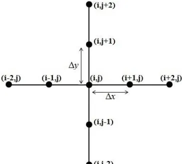
To illustrate the use of FD approximations, consider an elliptic PDE commonly encountered in computational mechanics (solid, fluid and heat transfer). Steady-state heat conduction, potential flow around a body, Prandlt’s stress function in an arbitrary bar and the streamfunction-vorticity formulation of the Navier-Stokes equations are some problems that are defined by elliptic PDEs. The 2nd-order accurate approximation of the elliptic Poisson equation ∇2∅ = 𝐹(𝑥, 𝑦) at an arbitrary node (i, j) of the uniform grid system shown in Figure 1.1 is written as

∅(i−1,j)− 2∅(i,j)+ ∅(i+1,j)

(∆𝑥)2 +

∅(i,j−1)− 2∅(i,j)+ ∅(i,j+1)

(30)

4

Figure 1.1: Uniform grid system used for solution of Poisson equation

The grid points used in this finite difference approximation of the Poisson equation at point (i, j), illustrated in Figure 1.1, constitute a five-point stencil. This stencil is the basic one for the cut-stencil FDM which will be discussed in Chapter 2. The solution of the Poisson equation in the grid system of Figure 1.1, in the event of Dirichlet boundary conditions, requires the solution to a system on (M-2)(N-2) algebraic equations. This system of equations can be cast into a matrix

form 𝐴Φ⃗⃗⃗ = 𝑏⃗ , in which 𝐴 is the matrix of coefficients, Φ⃗⃗⃗ is the vector of unknowns 𝜙(𝑖,𝑗) and 𝑏⃗ is the vector which incorporates the boundary values and the right hand side for each equation. The solution algorithms for matrix equations are divided into two main approaches, namely direct and iterative methods. Cramer’s rule, Gaussian elimination and LU-decomposition are well-known direct methods to solve a system of linear equations. Details for these direct solution algorithms can be found in Leslie and McAvaney [18] and in many textbooks on numerical linear algebra. Direct methods generally suffer from some disadvantages, especially when the matrices are not simple tridiagonal ones, and may not be computationally efficient. Additionally, the computational storage is huge especially for large size problems that are common in computational mechanics. Accumulation of round-off errors during the arithmetic calculations may also produce poor solutions and consequently a concerted effort should be made to reduce these errors [19, 20]. Due to these limitations, and non-linear coefficients for most PDEs of practical interest, direct methods, generally, are not used in the computational mechanics field. The following section presents a brief introduction to iterative methods which have been employed throughout this thesis to solve PDEs using the Cartesian cut-stencil FDM.

1.3.2 Iterative Solution Algorithms

(31)

5

FD solution to the PDEs. The cut-stencil FD solution for the streamfunction-vorticity formulation of the Navier-Stokes equation is presented in Chapter 5 by using the SUR method depending on the mesh size and Reynolds number. Thus, a brief explanation of these schemes is addressed here. Equation (1.3) is rewritten as

∅(i−1,j)+ ∅(i+1,j)− 2(1 + 𝛾2)∅(i,j)+ 𝛾2(∅(i,j−1)+ ∅(i,j+1)) = (Δ𝑥)2𝑓(𝑥i, 𝑦j) (1.4.1)

in which 𝛾 denotes Δ𝑥/Δ𝑦. Assuming that ∅(i,j)is known at a current iteration level k, i.e., ∅(i.j)𝑘 is known, the new value of the dependent variable at new iteration level 𝑘 + 1 at node (i, j) is calculated from

∅(i.j)𝑘+1=

∅(i−1,j)𝑘 + ∅(i+1,j)𝑘 + 𝛾2(∅𝑘(i,j−1)+ ∅(i,j+1)𝑘 ) − (Δ𝑥)2𝐹(𝑥i, 𝑦j)

2(1 + 𝛾2₎ (1.4.2)

The iterative formulation (1.4.2) is known as the Point-Jacobi method, which is regarded as the simplest iterative formulation. It is noted that P-J retains all values of the dependent variable from the old level of iteration until the calculation at level 𝑘 + 1 ends.

The point successive (under or over) relaxation version for calculation of the dependent variable at node (i, j) is expressed as

∅(i.j)𝑘+1 = (1 − 𝜎)∅(i.j)𝑘 +

𝜎[∅_(i−1,j)𝑘+1 _{+ ∅} (i+1,j) 𝑘 _{+ 𝛾}2_(∅

(i,j−1) 𝑘+1 _{+ ∅}

(i,j+1)

𝑘 _{) − (Δ𝑥)}2_𝐹(𝑥

i, 𝑦j)]

2(1 + 𝛾2₎ (1.4.3)

In point successive relaxation methods, the updated values of the dependent variable at neighboring nodes are immediately used for calculation of the dependent variable at node (i, j). The parameter 𝜎 in equation (1.4.3) is referred to as the relaxation parameter and the Gauss-Seidel method is recovered when 𝜎 = 1. The converged solution is obtained by implementing the condition 0 < 𝜎 < 2. The rate of convergence may be accelerated by changing the value of 𝜎. Computing an optimum value of relaxation parameter requires a procedure to solve an eigenvalue problem and it can only be applied to some limited cases, depending on the mesh scheme and type of boundary conditions. Some analytical suggestions and discussions for finding 𝜎𝑜𝑝𝑡 are available in numerical analysis literature [17, 23, 24].

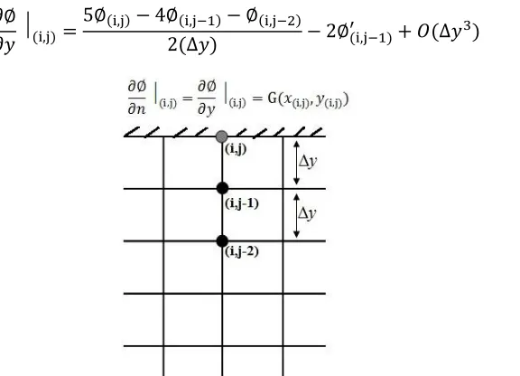
1.3.3 Ghost Node Method for Neumann Boundary Condition Treatment in TFDM

(32)

6

Figure 1.2: Schematic of grid system showing ghost node for approximation of imposed Neumann condition on the lower boundary

The 2nd-order central differencing approximation for the first derivative in the Neumann condition can be written using the fictitious node (i, 0). It is worth pointing out that in the grid system of Figure 1.2, values of 𝜙 at all the nodes located along the grid line j = 1 are unknown. To simplify the discussion, without losing generality, it is assumed that the outward normal vector to the boundary line, depicted in Figure 1.2, has a negative component along the 𝑦- direction, i.e.,

𝑛̂ = −ĵ, where ĵ is the unit normal along the 𝑦-axis in the Cartesian coordinate system. Then, the Neumann condition can be approximated as

𝜕∅ 𝜕𝑦⃒(i,1)=

∅(i,2)− ∅(i,0)

2(∆𝑦) = −G(𝑥, 𝑦)⃒(i,1) (1.5.1)

Using the same central differencing format as for the interior nodes, the governing equation (Poisson equation) at a typical boundary node (i, 1) with Neumann condition is given by

∅(i−1,1)− 2∅(i,1)+ ∅(i+1,1)

(∆𝑥)2 +

2∅(i,2)− 2∅(i,1)+ 2(∆𝑦)𝐺|(i,1)

(∆𝑦)2 = 𝐹(𝑥i, 𝑦1) (1.5.2)

where equation (1.5.1) has been used to eliminate the value of 𝜙 at the ghost node (i, 0). Similar to the case of Dirichlet boundary conditions, any of the iterative methods can be employed to solve for the unknowns, including those at the discrete points along the lower boundary.

(33)

7

1.4 Transformation of PDEs

As mentioned above, the TFDM is primarily employed for the numerical approximation of PDEs within regular shaped domains with a uniform grid system. In the case of irregular shaped domains, transformation of the physical domain (x-y space) to a regular (mostly rectangular shape) computational domain (𝜉 − 𝜂 space) is required. To accomplish this transformation, two main categories of approaches have been developed; algebraic methods and partial differential equation methods. Each has its own advantages and drawbacks [25]. The conformal mapping technique that is based on complex variables is an alternative method to generate a grid, but is restricted to 2-D applications [17]. A 2-D physical grid transformation to a computational one is illustrated in Figure 1.3.

Figure 1.3: Sample of a 2-D grid transformation, a) physical domain, and b) computational domain

Besides generating the grid for the domain of interest, the parameters that determine the quality of the generated grid, such as smoothness, skewness and orthogonality must be examined to ensure the appropriate level of accuracy for the solution of the mapped equations [26]. In fact, grid generation plays a significant role in yielding an accurate solution of e.g., flow passing bodies with irregular and complex shapes. It is known that the computed values and the solution properties are affected by the metrics of the generated grid [27]. Algebraic grid generation, the simplest and fastest technique [17, 28], cannot guarantee the orthogonality of the generated grid [29]. Orthogonality of the grid is associated with a number of advantages such as less number of terms in the transformed equations and more accurate interpolations. Additionally, the numerical accuracy of differencing schemes is higher and implementation of boundary conditions is carried out in a simpler way on an orthogonal grid [30, 31].

This implies that besides the computational and human effort that must be devoted to the grid generation procedure, each method may suffer from its own inherent difficulties. On the other hand, the Cartesian cut-stencil FDM, even in cases of complex and irregular shaped domains, does not depend on the grid generation in its formal and classical definition. This feature originates from a localized mapping of each physical stencil which may have uniform or non-uniform arm lengths. The details of the localized mapping will be presented in Chapter 2.

The remaining material of this section illustrates the transformation of a model governing PDE,

the convection-diffusion equation ∇2∅ + 𝑃𝜕∅_𝜕𝑥+ 𝑄𝜕∅_𝜕𝑦= 𝐹(𝑥, 𝑦), and introduces the mapped form

(34)

8

to reveal the differences between equation transformation in TFDM and in the Cartesian cut-stencil FDM, which will be introduced in Chapter 2. Consider the transformation functions

𝜉 = 𝜉(𝑥, 𝑦) and 𝜂 = 𝜂(𝑥, 𝑦) which, under the assumption that the Jacobian 𝐽 =𝜕(𝑥,𝑦)_{𝜕(𝜉,𝜂)} is non-zero,

uniquely map points from the x-y plane to points in the 𝜉-𝜂

plane.

Using the chain rule for partial differentiation, the first derivative operators can be expressed as:

𝜕 𝜕𝑥= 𝜉𝑥 𝜕 𝜕𝜉+ 𝜂𝑥 𝜕 𝜕𝜂 , 𝜕 𝜕𝑦= 𝜉𝑦 𝜕 𝜕𝜉+ 𝜂𝑦 𝜕 𝜕𝜂 (1.6.1)

where 𝜉𝑥 and 𝜉𝑦 denote the partial derivatives 𝜕𝜉_𝜕𝑥 and _𝜕𝑦𝜕𝜉 respectively, and similarly for 𝜂𝑥 and 𝜂𝑦.

The second derivative operators are transformed in the same fashion as:

𝜕2

𝜕𝑥2=𝜉𝑥𝑥

𝜕

𝜕𝜉+ 𝜉𝑥[𝜉𝑥

𝜕2 𝜕𝜉2+ 𝜂𝑥

𝜕2 𝜕𝜉𝜕𝜂]+ 𝜂𝑥𝑥 𝜕 𝜕𝜂+ 𝜂𝑥[𝜉𝑥 𝜕2 𝜕𝜉𝜕𝜂+ 𝜂𝑥 𝜕2

𝜕𝜂2] (1.6.2)

𝜕2

𝜕𝑦2=𝜉𝑦𝑦

𝜕

𝜕𝜉+ 𝜉𝑦[𝜉𝑦

𝜕2 𝜕𝜉2+ 𝜂𝑦

𝜕2 𝜕𝜉𝜕𝜂]+ 𝜂𝑦𝑦 𝜕 𝜕𝜂+ 𝜂𝑦[𝜉𝑦 𝜕2 𝜕𝜉𝜕𝜂+ 𝜂𝑦 𝜕2

𝜕𝜂2] (1.6.3)

The transformed model equation, from physical domain (space) to computational domain (space), using equations (1.6.1)-(1.6.3), can be expressed in the form

𝜉_𝑥𝑥𝜕∅

𝜕𝜉+ 𝜉𝑥[𝜉𝑥 𝜕2_∅

𝜕𝜉2+ 𝜂𝑥

𝜕2_∅

𝜕𝜉𝜕𝜂] + 𝜂𝑥𝑥 𝜕∅

𝜕𝜂+ 𝜂𝑥[𝜉𝑥 𝜕2_∅

𝜕𝜉𝜕𝜂+ 𝜂𝑥 𝜕2_∅

𝜕𝜂2] + 𝜉𝑦𝑦

𝜕∅ 𝜕𝜉

+ 𝜉_𝑦[𝜉_𝑦𝜕2∅ 𝜕𝜉2 + 𝜂𝑦

𝜕2_∅

𝜕𝜉𝜕𝜂] + 𝜂𝑦𝑦 𝜕∅

𝜕𝜂+ 𝜂𝑦[𝜉𝑦 𝜕2_∅

𝜕𝜉𝜕𝜂+ 𝜂𝑦 𝜕2_∅

𝜕𝜂2]

+ 𝑃 [𝜉𝑥 𝜕∅ 𝜕𝜉+ 𝜂𝑥 𝜕∅ 𝜕𝜂] + 𝑄 [𝜉𝑦 𝜕∅ 𝜕𝜉+ 𝜂𝑦 𝜕∅ 𝜕𝜂] = 𝑓(𝜉, 𝜂) (1.6.4)

From advanced calculus, one can write relationships between the metrics of the transformation:

𝜉_𝑥 = 𝐽−1_𝑦

𝜂, 𝜉𝑦 = −𝐽−1𝑥𝜂, 𝜂𝑥 = −𝐽−1𝑦𝜉, 𝜂𝑦= 𝐽−1𝑥𝜉 (1.6.5)

The application of such 2-D transformation functions has been discussed extensively in numerical studies of grid generation methods [32-35].

The comparison of the transformed form of the model equation, stated in (1.6.4), and the equation obtained using the specific transformation functions of the cut-stencil FDM, which will be discussed in Chapter 2, shows the obvious simplicity of the Cartesian cut-stencil FDM. The main reason for the simplicity of the mapped model equations in the Cartesian cut-stencil FD formulation arises from independent 1-D transformation equations which exhibit the necessary features of the localized mapping of each stencil.

1.5 Cartesian Grid