Evaluating the Augmentation of Army Resupply with Additive Manufacturing in a Deployed Environment.

(1)

ABSTRACT

MOORE, TIMOTHY ANDREW. Evaluating the Augmentation of Army Resupply with Additive Manufacturing in a Deployed Environment. (Under the direction of Dr. Thom Hodgson.)

This thesis models the problem of keeping a M109A6 operational while in a deployed environment, comparing traditional resupply methods to additive manufactured spare parts. The additive technology is co-located with the howitzer unit, establishing a decentralized supply chain. Specifically, what conditions make it advantageous to deploy additive manufacturing technology to produce spare parts printed on demand? This model can assist decision makers determining when to augment a unit’s typical safety stock with a 3D printing facility that can satisfy a howitzer unit’s demand rate while deployed comparing cost and lead-time to make the best decision possible.

The model utilizes MATLAB to perform a simulation on the parts request process. In particular, the model was constructed so that different parameters could be manipulated based off of preference from the decision maker. For instance, the demand rate can easily be increased or decreased to simulate different phases of an operation or different environments altogether. For the purposes of this paper only parts comprised of metal were considered in the demand rate because those parts directly impact the validity of utilizing a Direct Metal Laser Sintering (DMLS) printer. Secondly, the model incorporates fixed and variable costs to demonstrate the fiscal

requirements to implement such a program. Again, the parameters within the cost model can easily be adjusted to accurately reflect competitive pricing for the additive equipment and it can also be adjusted based on the unit size that the additive equipment is required to support.

Once the tools were built, it painted a realistic scenario for what conditions needed to be satisfied for additive capability to be useful in a deployed environment. This analysis enhances decisions that directly impact the capabilities of Soldiers in the most dire of situations: combat. The goal of this thesis is to highlight the areas that need to be focused on within additive manufacturing to become a realistic option for the military to adopt its technology. Ultimately, additive

(2)

(3)

Evaluating the Augmentation of Army Resupply with Additive Manufacturing in a Deployed Environment

by

Timothy Andrew Moore

A thesis submitted to the Graduate Faculty of North Carolina State University

in partial fulfillment of the requirements for the Degree of

Master of Science

Operations Research

Raleigh, North Carolina 2018

APPROVED BY:

________________________________ ________________________________ Cecil Bozarth Russell King

________________________________ Thom Hodgson

(4)

ii

DEDICATION

(5)

iii

BIOGRAPHY

Tim Moore was born and raised in Roanoke, VA before attending college at the United States Military Academy at West Point, where he received a B.S. in Economics in 2008. Upon

commissioning as a Field Artillery Second Lieutenant in the United States Army he served as a Platoon Leader and Company Fire Support Officer while deploying in support of Operation Iraqi Freedom. He would go on to serve as a Battalion Fire Direction and Battalion Fire Support Officer while deploying in support of Operation Enduring Freedom in Afghanistan. He commanded in the 1st Brigade 41st_{Field Artillery Regiment at Fort Stewart, GA and completed two training rotations to} Europe in conjunction with our NATO partners. In the summer of 2016 he began to study Operations Research at North Carolina State University and upon completion he will be assigned to the

(6)

iv

ACKNOWLEDGEMENTS

(7)

v

LIST OF TABLES

Table 3-1. Build Time Data based on Volume ... 21

Table 5-1. Baseline Data drawn from original RAND demand data. ... 34

Table 5-2. Simulation results decreasing the allowable part size. ... 35

Table 5-3. Simulation results holding demand and allowable part size constant. ... 36

Table 5-4. Simulation results decreasing the demand rate. ... 36

Table 5-5. Factors for Simulations ... 37

Table 5-6. Factorial Design Points for Simulations ... 37

(10)

viii

LIST OF FIGURES

Figure 3-1. Organization of Requisition Data ... 16

Figure 3-2. Number of Orders Per Day ... 17

Figure 3-3. Goodness of Fit ... 18

Figure 3-4. Fitted Density... 18

Figure 3-5. Fitted Distribution ... 18

Figure 3-6. Autocorrelation of Orders Per Day ... 19

Figure 3-7. AM Build Process ... 20

Figure 3-8. Regression Data Using R Software ... 22

Figure 3-9. Linear Regression of Build Times Based on Volume ... 23

Figure 3-10. Simulation Process ... 25

Figure 3-11. Total Cost Breakdown ... 28

Figure 4-1. Requisition Simulation Process ... 29

(11)

ix

LIST OF EQUATIONS

Equation 1. Baumers Build Time Estimation Formula ... 21

Equation 2. Simple Linear Regression Model ... 21

Equation 3. Design Costs ... 25

Equation 4. Setup Costs ... 26

Equation 5. Material Costs ... 26

Equation 6. Production Costs ... 27

Equation 7. Post-Production Costs ... 27

Equation 8. Total Cost Formula ... 27

Equation 9. Beta Distribution (min, max, p, q) ... 31

(12)

1

Chapter 1. INTRODUCTION

1.1 Additive Manufacturing

Additive manufacturing (AM) came to light in the 1980’s but has recently garnered the attention of industry and hobbyists alike as a potentially time and cost effective way to make products. The accessibility of 3D printing continues to broaden and the technology itself continues to become more proficient and less expensive. The Economist recently went so far as to tout AM as a “third industrial revolution” that has the potential to change manufacturing on a global scale (Whadcock, 2012). People looking to experiment in their homes have certainly bought in, eager to exploit the new technology. In Wohler’s Report 2016, desktop 3D printer unit sales (less than $5,000) grew at an astounding 69.7% in 2015, selling 278,385 machines (Wohlers, 2016 ). As Malcolm Gladwell put it, “there is a simple way to package information that, under the right circumstances, can make it irresistible” and 3D printing has certainly intrigued many (Gladwell, 2000). A tipping point is fast approaching where AM becomes widely used to augment product manufacturing.

AM application in a military context could be widely beneficial, allowing for a faster and potentially cheaper resupply of requested spare parts by simplifying the supply chain and reducing inventory costs. The military lends itself to the adoption of AM because it frequently operates in hazardous locations that naturally isolates its Soldiers from logistical resupply. In this scenario, the military stands to gain the most from AM technology and it therefore deserves to be analyzed as a practical option to augment traditional resupply methods.

1.2 Define the Problem

Like all companies, the military wants to save money when possible without cutting corners.

(13)

2

1.3 Objectives

This thesis provides a synopsis of all current AM studies in the literature review, highlighting many of the advantages this technology can provide. The thesis goes on to describe a process, simulation, for evaluating the feasibility of augmenting an Army supply chain with AM technology. The demand data for parts requested was taken from actual units in Iraq during the US’s initial invasion.

Specifically, a M109A6 Paladin’s parts are analyzed to reflect a realistic demand rate for just one end item. In this case, the Paladin is a self-propelled howitzer and is the main weapon system for a mechanized artillery unit. This data is manipulated through a series of assumptions and fed into a computer simulation in order to analyze the results. Lastly, these results are incorporated in realistic recommendations for how the Army can potentially improve its supply chain practices.

(14)

3

Chapter 2. LITERATURE REVIEW

The current consensus is that there are enormous advantages to harnessing the capabilities of AM and many scholars have written extensively on this topic. The literature review aims to provide a cogent synopsis of all relevant work that has been done on the implications of additive

manufacturing in order to highlight the research gap between well-structured costs analysis and those of the ill-structured variety. Well-structured costs consist of material, labor, and

manufacturing system costs (Young, 1991). Ill-structured costs stand as the areas which can benefit the military the most: transportation and inventory costs.

2.1 Current State of Additive Manufacturing

AM at its simplest is the process of joining materials to make objects from 3D model data, usually layer upon layer, as opposed to subtractive manufacturing methodologies. The oldest technology, Stereolithography (SLA), uses a photosensitive resin and exposes it to a UV laser beam to create the product. The most common form of 3D printing is Fused Deposition Modeling (FDM) where a thermoplastic filament is heated and melted layer by layer in the X/Y direction and lowered in the Z direction. An emerging technology is Electron Beam Melting (EBM) that allows highly durable metals to be formed under an electron beam in a high vacuum that melts the metal powder. For this thesis, Direct Metal Laser Sintering (DMLS) is considered as the main AM technology. DMLS uses lasers to fuse powdered metals into functional prototypes and end-use parts. The key understanding is that AM technology is constantly improving and evolving so it is reasonable to expect that higher quality products will be created more quickly and less expensively in the future.

(15)

4

The fascination is warranted because AM allows for the creation of completely redesigned products: lighter weight with new strength properties, combination of multiple parts into one, or rapidly decreasing the time required to make a prototype into a reality. In a recent example, Amaero and Monash University were able to make multiple prototypes of a rocket engine, tweaking complex geometrical details, and save months of design time (Haria, 2017). However, in most circumstances the technology is not low-cost enough and cannot produce products quickly enough to immediately replace traditional manufacturing (TM). Nearly all academic studies up to date agree that AM technology will serve best as a complement to machining rather than an outright replacement for the foreseeable future (Bogers, Hadar, & Billberg, 2015). Despite that, the desire for AM to become the primary production method is heavily present in many sectors and the companies that begin to explore the uses of AM now will benefit the most later, once AM technology catches up to the demand levels that TM currently satisfies.

One important factor to note about the AM industry is that a lot of companies that produce the technology also own the raw materials to be able to print with AM. This creates a partially skewed market because the suppliers do not face as much competition as they would if it were a well-established technology. In the future, it is expected that more companies will enter the AM production field, thus driving prices down to a more a competitive rate.

There are still many obstacles that prevent companies from adopting and implementing AM in their own production processes. The largest problem is that AM simply cannot keep pace with large volumes of demand. Regardless of how inexpensive the technology becomes, build times will have to decrease drastically in order to produce at a rate sufficient for products in high demand. Another hindrance that often gets overlooked is having the correct personnel in place to ensure that AM is run properly. Not just anyone can hit “print” and be done with the production process. Highly specialized engineers are required to create Computer Assisted Drawings (CAD) that serve as blueprints for products being created through AM. Another large obstacle is maintaining the physical printers as well as the quality of the products that are being printed. Again, existing personnel would have to be trained on the AM technology or replaced altogether.

2.2 Background

The rise of 3D printing and additive manufacturing will replace the competitive dynamics of

(16)

5

some industries and products (Petrick & Simpson, 2013). Areas that stand to gain the most from AM include: 1) Mass customization, 2) Resource efficiency, 3) Decentralization of manufacturing, 4) Complexity reduction, 5) Rationalization of inventory and logistics, 6) Product design and prototyping, and 7) Legal and security concerns (Mohr & Khan, 2015). Each of these areas are explained in depth with relevant literature that supports the advantages of implementing AM and relevant case studies that highlight some of these areas are further explained.

2.2.1 Ill-Structured Costs

Much of the relevant AM research that has been conducted does not accurately explain the potential benefit that AM can provide to ill-structured costs. Ill-structured costs are generally comprised of supply chain aspects. Inventory is a primary example of an ill-structured cost that provides tremendous upside for AM technology. The resources spent producing and storing these products could have been used elsewhere if the need for inventory were reduced. Suppliers often suffer from high inventory and distribution costs. Additive manufacturing provides the ability to manufacture parts on demand. Traditional production technologies make it too costly and require too much time to produce parts on demand. The result is a significant amount of inventory of infrequently ordered parts. This inventory is tied up capital for products that are unused. They occupy physical space, buildings, and land while requiring rent, utility costs, insurance, and taxes. Meanwhile the products are deteriorating and becoming obsolete. Being able to produce these parts on demand using additive manufacturing reduces the need for maintaining large inventory and eliminates the associated costs (Gilbert & Thomas, 2014).

In an (s-1, s) inventory model for spare parts, Sirichakwal & Conner demonstrated that the concept of virtual inventory, made possible by AM, has many appeals for spare parts inventory management especially in systems where inventory obsolescence and stock-out risk are of high importance. They also showed that a reduction in holding cost has more impact on reducing the stock-out probability when the average demand rate for spare parts is low. Additionally, lead time reduction can actually have a negative impact on the stock-out probability (Sirichakwal & Conner, 2016).

Transportation is another huge aspect of the supply chain that AM technology looks to alter drastically in the future. Additive manufacturing allows for the production of multiple parts simultaneously in the same build, making it possible to produce an entire product in one step. Traditional manufacturing often includes production of parts at multiple locations, where an

(17)

6

into a product. Additive manufacturing has the potential to replace some of these steps for some products, as this process might allow for the production of the entire assembly in one build. This would reduce the need to maintain large inventories for each part of one product, reduce the transportation of parts produced at varying locations, and reduce the need for Just-In-Time (JIT) delivery (Thomas, 2016). Another substantial transportation impact is the location of the production facility which can be nearer to the user and is described in detail in its own section due to its

importance.

2.2.2 Supply Chain

The supply chain includes purchasing, operations, distribution, and integration. Purchasing involves sourcing product suppliers. Operations involve demand planning, forecasting, and inventory.

Distribution involves the movement of products and integration involves creating an efficient supply chain (Robinson, 2015). AM provides the potential for many advantages in the manufacturing supply chain. A noticeable benefit is dematerializing the supply chain itself. If there are fewer steps along the chain, then efficiency increases and the chance for delays and disruptions decreases. Other advantages include true Just-In-Time manufacturing, reduced set up, changeover time, number of assemblies, and the elimination of waste (material, time, costs, distribution) (Tuck, Hague, & Burns, 2007). AM also enables JIT manufacture at the shop floor instead of JIT delivery of supplies to the shop floor. As a result, non-value added activities such as material movement and inventory holding can be reduced to a minimum. The result is a lean supply chain with low cost. Additionally, AM can improve the responsiveness of an agile supply chain. A build-to-order strategy can be implemented to ensure that no stockout would occur. The overriding cost for AM production is not labor but the machines and raw materials, which makes it economical to locate production facilities near the end customers. Lastly, it is possible to customize products to meet individual customer needs. This will facilitate the implementation of a build-to-order strategy and increase responsiveness to customer’s demands (Huang, Liu, & Mokasdar, 2013).

All businesses aim to be efficient at every level and collectively the industry has adopted the 6 Sigma approach towards a lean and agile supply chain. Thomas et al (2014) described seven categories for a company to focus on in order to become lean:

(18)

7

2) Transportation: transportation does not make any change to the product and is a source of risk to the product

3) Rework/Defects: discarded defects result in wasted resources or extra costs correcting the defect

4) Over-processing: occurs when more work is done than is necessary

5) Motion: unnecessary motion results in unnecessary expenditure of time and resources 6) Inventory: is similar to that of overproduction and results in the need for additional handling, space, people, and paperwork to manage extra product

7) Waiting: when workers and equipment are waiting for material and parts, these resources are being wasted

AM has the potential to improve efficiency for each of these tenets.

Manufacturing and delivering products to customers require the efforts of various companies that form the manufacturing supply chain. These companies may include raw material suppliers, component suppliers, original equipment manufacturers, wholesalers/distributors, logistics service providers, and retailers. In a supply chain, materials flow forward from suppliers through various stages toward customers, whereas information and funds flow backward. As described, AM has the potential to reduce the number of stages in the traditional supply chain. Specifically, AM technology offers two opportunities: (1) to redesign products with fewer components and (2) to manufacture products near the customers (i.e., distributed manufacture). The net effect is reduction in the need for warehousing, transportation, and packaging (Huang, Liu, & Mokasdar, 2013). These elements combined illustrate the enormous impact AM technology can bring to the manufacturing supply chain.

Hasan and Rennie (2009) noted that a fully functional AM supply chain was not yet available in 2009 in the spare parts industry. The authors proposed a business model to enable such a supply chain. The model is based on an e-business platform that provides the following services (Hasan & Rennie, 2009):

1) Sourcing: give buyers easy access to a pool of suppliers.

(19)

8

3) Content display: provide an e-catalogue to display the products and services provided by the suppliers.

4) Transaction: enable the exchange of procurement information between the buyers and suppliers.

5) Promotion: help suppliers advertise their products and services.

2.3 Advantages/Disadvantages

2.3.1 Pros

This section consolidates the benefits of AM for particular industries to utilize. AM technology is constantly evolving and the upside is seemingly limitless (Steenhuis & Pretorius, 2017). AM opens opportunities for manufacturing companies in three regards: 1) AM offers the option of generating objects that would have been impossible to make with any other technology, 2) AM can be used as an automation technology which substitutes for human labor, and 3) AM allows for cost-efficient switching from traditional mass production to new areas of mass customization (Thiesse, Wirth, & Kemper, 2015).

As a result of Niaki & Nonino (2017), we can affirm that AM brought not only a process innovation but also product innovation. This revolutionary technology allows for the fabricating of creative products and construction of highly complex parts; sharing design and collaboration with consumers with a low cost of modifications; enabling the full customization of parts with more functionality and aesthetic appeal, which is impossible for general production to fabricate with traditional techniques. In addition to introducing new products, AM leads to new markets. Therefore, it is reasonable to expect a growing demand for AM as some firms in the study have found, as well as an increasing willingness of consumers to pay more for the higher value offered. This higher value is influenced by customer service through time-to-market reduction and full customization, and provides the

possibility to charge higher prices, especially for parts made in metal. Consequently, it influences revenue in a positive way and is an attractive investment (Niaki & Nonino, 2017).

Another advantage is a simplified supply chain to increase efficiency and responsiveness in demand fulfillment. AM is conducive to innovative design and enables on-demand manufacturing. As a result, the need for warehousing, transportation, and packaging can be reduced significantly. With proper supply chain configuration, it is possible to improve cost efficiency while maintaining

(20)

9

true where customers can obtain desirable products economically whenever they want and without leaving their homes (Huang, Liu, & Mokasdar, 2013).

Many specific case studies conducted include multiple different types of industry and reflect the effect of AM’s benefits in their results. Hearing aid companies in particular have been one of the most prevalent adopters of AM. In a specific case study, a hearing aid company bought AM

technology and produced parts in house instead of by a third party. Although the company needed highly paid engineers to build the designs, new benefits far outweighed this downside. In fact, the company accomplished this by emailing scanned ear canals to a company in Germany that already had CAD model engineers. Since the CAD designs were now being sent electronically the process allowed for distributed manufacturing. This scenario reduced lead time by eliminating physical deliveries (email request of scanned ears). Overall, both companies in this case study were able to increase material utilization and improve efficiency (Oettmeier & Hofmann, 2016). In another empirical case study on a lamp company, the results showed the supplementary capacity of the AM process and how it improved the supply chain (SC) performance in terms of lead time and total cost. That work identified the research gap between AM and SC and gave a comprehensive investigation of different performance indicators such as order fulfill rate and waste rate (Chiu & Lin, 2015). Another case study described many of the themes highlighted in this section. Specifically, General Motors offers a program called Retail Inventory Management (RIM) that allows dealers to return parts that do not sell in 15 months without any penalty. While the dealership avoids paying for the part, they still have money tied up in labor costs to stock the part, rent utilities, taxes, insurance, and the opportunity cost associated with carrying the part. It is easy to see that a dealership which implemented AM of parts on demand could significantly reduce

1) the type and quantity of spare parts needing to be stocked

2) procurement costs for parts the dealer would typically order from the manufacturer or another location

3) shipping costs for parts ordered as well as obsolete parts returned 4) costs involved in recall programs for malfunctioning parts

(21)

10

drastically for selected parts but lead time has been significantly reduced as well. One example of a component transformed by AM was a “liftgate badge tool” which is used to precisely place the car’s logo. Lead time dropped 89%, with outsourcing taking an average of 35 days and 3D printing just 4 (Jackson, 2017).

Lastly, in England two different types of companies were analyzed: wallpaper and chemical filter suppliers. The decoupling point was moved upstream to allow for high levels of customization which greatly enhanced the perceived value by customers. Through the adoption of AM, additional

processes resulted in value stream (VS) creation, which co-existed with existing VSs to enhance and strengthen manufacturing (without replacing traditional methods or VSs). This provided both companies with the ability to grow their business and capabilities further to compete, positively impacting on their region with spillover of skill, knowledge and economic benefit (Rylands, Bohme, Gorkin, Fan, & Birtchnell, 2016). The case study resulted in the following hypotheses:

1) Incorporating AM into the manufacturing system results in growth across VSs due to close client engagement during the co-creation process.

2) AM is not replacing existing manufacturing/VS, rather it is complementing a company’s offerings.

3) Unless the VS changes, the business impact is limited (engineering solutions rather business solutions).

4) AM knowledge centers are critical supply chain nodes for a company pull driven implementation process.

2.3.2 Cons

Many barriers still exist to the adoption of AM and it is important not to discount these aspects and get swept up in the potential benefits. The results suggest the AM machine acquisition price and personnel intensiveness are major obstacles to a distributed deployment of this technology in spare parts supply chains (Khajavi, Partanen, & Holmstrom, 2014).

Another study reveals a number of disadvantages and challenges ahead of this emerging

(22)

11

suppliers lead to a high negotiating power for AM material suppliers, in spite of efforts to develop new viable materials (Hao, Zhang, & Mellor, 2014) (Niaki & Nonino, 2017).

2.4 Centralized vs. Distributed

As mentioned above, the largest potential for a disruptive change in supply chain management is the location of production. Holmstrom et al. (2010) proposed two different approaches to integrate AM technology in the spare parts supply chain. The first approach is to use centralized AM capacity to replace inventory holding. AM machines are deployed in centralized distribution centers to produce slow-moving spare parts on demand. Producing parts in a centralized location has the advantage of aggregating demand from various regional service locations to ensure that the investment in AM capacity is well utilized. The disadvantage is that the produced parts need to be shipped to the service locations, which results in an increase of response time. A method to mitigate this issue by locating production at third party logistics (3PL) sites. Hence, once a part is printed it can be immediately shipped to its final destination (D'Aveni, 2015). However, for certain parts that are needed in the first line maintenance, inventory still needs to be carried in the service locations. The centralized approach is desirable when parts produced using AM are limited and the required response time is not critical. The second approach, distributed AM at each service location, is suitable when the demand of AM producible parts is sufficiently high to justify the capacity investment. The advantage of the distribution of AM is the elimination of inventory holding and transportation costs and a fast response time. In addition to these two approaches, Holmstrom et al. (2010) also contemplates the feasibility of mobile AM but concedes that there are many challenges. The authors further discusses the trade-off between batch production and on-demand production, and the trade-off between specialized and general purpose AM. The key variables considered are materials and production costs, distribution and inventory obsolescence costs, and life-cycle costs for the user. They concluded that on-demand and centralized production of spare parts is most likely to succeed (Holmstrom, Partanen, Tuomi, & Manfred, 2010).

In a case study conducted on aircraft spare parts, it is shown that the advantages of AM technology can be introduced into different stages of the aircraft spare parts supply chain. Again, the

(23)

12

because in this case the benefit of demand aggregation in a centralized distribution center is greatly diminished. It can also be used for parts with very short manufacturing lead time, especially if their demand is low and unpredictable; because such parts can be produced on-demand. It is clearly demonstrated that AM has the potential to change the conventional supply chain configuration. In this industry it is possible to achieve inventory reduction, thus cutting inventory holding costs across the entire supply chain (Liu, Huang, Mokasdar, Zhou, & Hou, 2014).

The potential advantages of using AM machines for the distributed production of aircraft spare parts can be summarized as follows: lower overall operation costs, lower down time, higher potential for customer satisfaction, lower capacity utilization, higher flexibility, fewer supply chain disruptions, reduced need for inventory management and logistics information systems, and potential for sustainability improvements as AM machines become smaller and more energy efficient (Khajavi, Partanen, & Holmstrom, 2014). However, the same study identifies notable gaps that prevented a distributed approach. To combat this, it was suggested that higher automation, lower acquisition price, and shorter production time of AM machines are the factors that the producers of these machines should aim to develop to enable radical change in spare parts supply chain operations (Khajavi, Partanen, & Holmstrom, 2014).

Decentralized distribution can remain challenging to fully realize. In another study a company is unable to do decentralized production because they do not have a consistent customer base, therefore cannot predict where they are going to sell their product. As a result, post-production processes and costs are high so decentralization would only increase costs (Hao, Zhang, & Mellor, 2014).

2.5 Direct Manufacturing

(24)

13

the same product that Hopkinson and Dickens produced using selective laser sintering (Ruffo, Tuck, & Hague, 2006). The cost model constructed in a more recent paper for EBM and DMLS

demonstrates that machine productivity forms a main driver of per-unit manufacturing cost. It also suggests that this contributes to a general cost barrier to technology diffusion of AM into

mainstream manufacturing (Baumers, Dickens, Tuck, & Hague, 2016). All these studies and others have to led to the conclusion that there is a value to be placed on the speed, versatility, and adaptability of AM as it allows for just-in-time manufacturing. Further, AM is favored in small production lots in which the higher cost of AM specific raw materials is offset by a reduction in fixed costs associated with conventional manufacturing (Frazier, 2014).

2.6 Ideal Candidate to Adopt

AM appeals to many different industries and in particular, ones that suffer from a natural divide from their customers and suppliers. For instance, space is a readily cited example for obvious reasons: distance to a supply depot! Other forms of isolation are encountered when the machine or blueprints required to produce an old part do not exist anymore. Additionally, a customer may be isolated due to a hazardous location, i.e. a war zone (Peres & Noyes, 2006).

Although AM technology has yet to be truly incorporated into the spare parts supply chain, it has been successfully used to supply certain consumer goods. Reeves (2010) described four such businesses that have adopted AM: (1) Fabjectory that enables players of Second Life to purchase models of individualized avatar characters, (2) FigurePrints that allows players of World-of-Warcraft to order 1/16th scale models of their online gaming characters, (3) Landprint that offers

(25)

14

(26)

15

Chapter 3. DESCRIPTION OF DATA

3.1 Data Used

3.1.1 Data Sources

All of the demand data used in this paper was provided by RAND Corporation (Peltz, Halliday, Robbins, & Girardini, 2005). The provided data displayed all part requisitions for Operation Iraqi Freedom (OIF) during a 162 day period that spanned the initial invasion in 2003. Each requisition within the data set had specific information pertinent to the entire supply process and a sample of the data is provided in Appendix A.1. The most important pieces of information for this thesis included quantity, weight, volume, price, request date, and delivery date. An important distinction is the requisition data does not reflect true demand because it is supply side data, not consumption data. Considering this data comes from OIF, it is plausible that units ordered parts based off not only actual needs but projected needs as well. Ultimately, the requisition data used in this thesis is more conservative comprising of supply side data.

Another data source was build time data. This was collected from MakerBot™ Thingiverse, an online design community for discovering, making and sharing 3D printable things. Specifically, 53 different products were selected that directly reflected build time and volume, Appendix A.2. The metal parts were all built using Direct Metal Laser Sintering (DMLS) and ranged from simple to complex designs. The parts varied enough to accurately reflect eventual Paladin part CAD models given that current blueprints do not exist for Paladin spare parts. However, the data range was limited to smaller parts, not fully reflecting all sizes of Paladin parts.

3.1.2 Data Organization

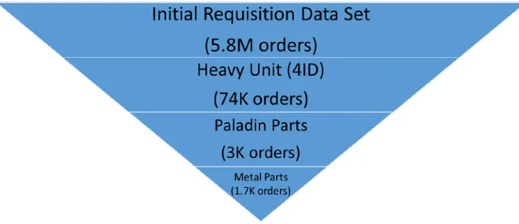
The requisition data was organized by only focusing on specific Unit Identification Codes (UIC) to determine what parts were ordered by heavy artillery battalions (BNs). To manage the scope of data points, 4th_{Infantry Division (4ID) was selected so only artillery BNs in 4ID are reflected in the data. It} is important to note that there were 3 artillery battalions requesting parts in the data set. The goal was to have a list of Paladin spare parts requested during this 162 day period but the given data set did not provide what end item (piece of Army equipment) each National Item Identification Number (NIIN) corresponded to. In order to solve this problem, a heavy artillery battalion’s monthly

(27)

16

specifically for a Paladin. The 4ID OIF data was scrubbed based off of the DCR which resulted in a list of Paladin parts that were requested during the first 162 days of OIF. Lastly, this list was filtered once more to only reflect spare parts made primarily of metal so that the demand rate used in the simulation model was solely for M109A6 Paladin spare parts made of metal during the first 162 days of OIF, Figure 3-1.

Figure 3-1 Organization of Requisition Data

3.1.3 Data Cleansing

Preparing the data was fairly straightforward for this data set. The first step was to eliminate erroneous orders. This was accomplished by filtering the orders and changing any order for a quantity of 0 to a quantity of 1. The assumption was made that if a supply clerk submitted the order then at least 1 part was required. This means part quantity is always greater than equal to 1, not to be confused with orders by day. There were multiple days during the 162 day period that no orders were submitted. The next step was to augment the request and delivery dates to reflect a more intuitive time. The supplied dates were provided with a Julian prefix for 2003, ex. 3053 represented February 22nd_{, 2003. So 3000 was subtracted from all dates for easier interpretation.}

3.2 Converting to Model Input

3.2.1 Arrival Rate (λ(t))

(28)

17

analyzed using StatFit2 and the descriptive statistics are displayed in Figure 3-2. Again, 162 (data points) days were used and the data reflects that a maximum of 98 orders in one day were made and mode of 7 orders a day occurred most frequently.

Figure 3-2 Number of Orders Per Day

(29)

18

Figure 3-3 Goodness of Fit

Furthermore, the fitted density and distribution reflect that Weibull is an acceptable distribution to generate random variables, Figure 3-4 & Figure 3-5.

Figure 3-4 Fitted Density

Figure 3-5 Fitted Distribution

(30)

19

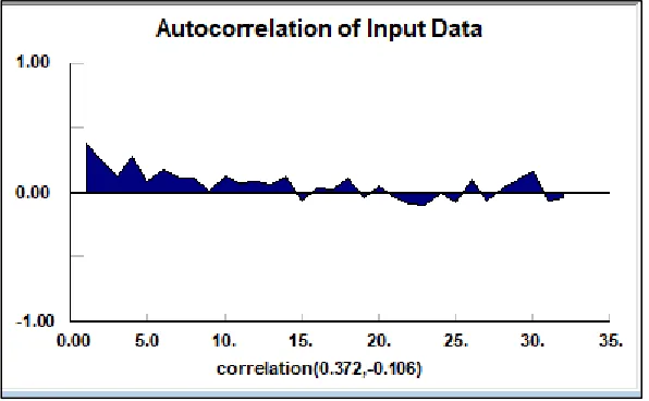
the auto-correlation data because none of the data is highly correlated, meaning the previous day does not have a significant impact on the amount of orders made the next day.

Figure 3-6 Autocorrelation of Orders Per Day

The arrival rate (λ(t)), number of orders per day, in this thesis varied based off the scenario the simulation was performing. For instance, the demand rate changed when different unit sizes were considered. Since the original data was reflective of 3 battalions making order requests, the demand rate decreased as the unit sizes decreased. All of the subsequent distribution fittings can be seen in Appendix D for reference. Additionally, all of the different scenarios are described and displayed in Chapter 5.

3.2.2 Service Rate (μ)

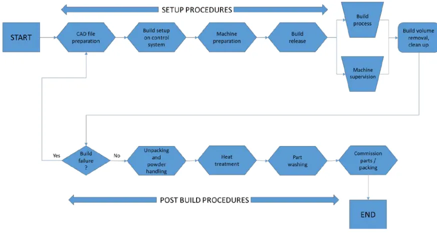
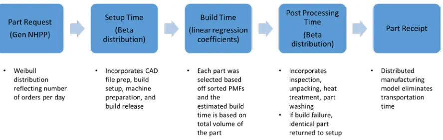
The first factor that needs to be satisfied to determine viability of AM implementation is for the production rate to meet the demand rate. This was accomplished by creating a simulation in MATLAB that kept track of the total sojourn time for requisitioned parts and discussed in further detail in Chapter 4. Figure 3-7 provides a depiction of all factors that were considered in the build time model. It is important to understand the entire process to accurately reflect the amount of time it takes to print a part.

3.3.2.1 Setup Procedures

(31)

20

of the steps occurring during the setup phase were accounted for with a Beta distribution which is described later in this section. This was selected because realistic bounds on setup times exist for every 3D build.

Figure 3-7 AM Build Process

3.3.2.2 Build Procedures

The actual build time estimation, given all necessary information about the CAD model, can be calculated precisely. In fact, there are many published papers that fully and accurately provide formulas to estimate build time for additive manufacturing. Equation 1 describes a globally accepted algorithm for estimating build times (Baumers, et al., 2012)

1) Fixed time consumption per build operation, 𝑇𝑇𝐽𝐽𝐽𝐽𝐽𝐽

2) Total layer dependent time consumption, obtained by multiplying the fixed time consumption per layer, 𝑇𝑇𝐿𝐿𝐿𝐿𝐿𝐿𝐿𝐿𝐿𝐿, by the total number of build layers 𝑙𝑙

3) The total build time needed for the deposition of part geometry approximated by the voxels. The triple Σ operator in Figure 3 expresses the summation of the time needed to

(32)

21 𝑇𝑇𝐵𝐵𝐵𝐵𝐵𝐵𝑉𝑉𝐵𝐵 = 𝑇𝑇𝐽𝐽𝐽𝐽𝐽𝐽+�𝑇𝑇𝐿𝐿𝐿𝐿𝐿𝐿𝐿𝐿𝐿𝐿 ×𝑙𝑙�+ � � � 𝑇𝑇𝑉𝑉𝐽𝐽𝑉𝑉𝐿𝐿𝑉𝑉 𝑉𝑉𝐿𝐿𝑥𝑥 𝑉𝑉 𝑉𝑉=1 𝐿𝐿 𝐿𝐿=1 𝑥𝑥 𝑥𝑥=1

Equation 1. Baumers Build Time Estimation Formula

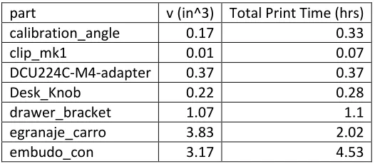
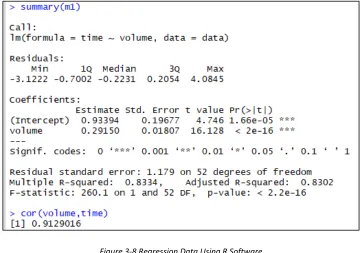
Baumers (2012) is referenced to acknowledge that there is a sophisticated approach to estimating build times. It is understood on a more simplistic level that build time is a function of the deposition speed and the length of the deposition in each layer. Additionally, the speed is certainly affected by the quality of the printer and the complexity of the part. However, all of these variables could not be captured for Paladin parts that do not currently have CAD models so the assumption was made that build time could be calculated given part volume. The statistical significance of this assumption is reinforced by the linear regression in Figure 3-9. The previously mentioned Thingiverse data reflected actual build times with their corresponding volumes, Appendix A.1.

Table 3-1 below shows a sample of the parts selected for the regression. Table 3-1 Build Time Data based on Volume

part v (in^3) Total Print Time (hrs)

calibration_angle 0.17 0.33

clip_mk1 0.01 0.07

DCU224C-M4-adapter 0.37 0.37

Desk_Knob 0.22 0.28

drawer_bracket 1.07 1.1

egranaje_carro 3.83 2.02

embudo_con 3.17 4.53

The regression was based on the following model in Equation 2.

𝑦𝑦= 𝛼𝛼+ 𝛽𝛽𝛽𝛽+ 𝜀𝜀

y = PartBuildTime α = intercept β = scalar x = PartVolume ε = error term Equation 2. Simple Linear Regression Model

(33)

22

multiplied by the known covariate, 𝑃𝑃𝑃𝑃𝑃𝑃𝑃𝑃𝑃𝑃𝑃𝑃𝑙𝑙𝑃𝑃𝑃𝑃𝑃𝑃, plus an error term (ε). The error term is assumed to be independently and identically distributed N(0,𝜎𝜎2_)._{The regression}_{fitted an α}_{parameter of}

0.93994 and β parameter of 0.29150 with an R2_{value of 0.8334, seen in}_{Figure 3-8}_._{Figure 3-9}

displays the 53 points of build time data regressed using R software. Time is displayed in hours and volume is in cubic inches. The regression’s intercept was not forced to 0 so that the model could more accurately predict small volume build times.

(34)

23

Figure 3-9 Linear Regression of Build Times Based on Volume

The volume for each Paladin part was plugged into the regression described above to get the build time for each part. Of note, print speed can be optimized in a chamber if small batches are created and products are printed simultaneously in the horizontal direction. This of course requires available space in the chamber and identical raw material between parts. This level of fidelity was not

possible for the build time model in this thesis so it was assumed that only one part would be built at a time.

3.3.2.3 Post Build Procedures

Now that the build process is complete, the printed part needs to be removed from the chamber. Routine cleaning inside of the chamber would be conducted by the engineer once the product has been removed.

(35)

24

increase the cost in the following cost model because additional material is used. In discussions with the Center for Additive Manufacturing and Logistics (CAMAL) at NC State, the assumption was build failure occurs at a 10% rate.

However, if the part passes inspection then post build procedures would commence. Although technology is improving rapidly, nearly all metal parts would have to undergo some kind of post-treatment to finalize the production process. An emerging technology to augment finishing of metal parts is Additive systems Integrated with subtractive Methods (AIMS). This is exciting technology because the subtractive techniques replicate traditional finishing techniques. This method would require custom tooling and fixtures but could be operated by one engineer (Manogharan, Wysk, Harrysson, & Aman, 2015). For this model, heat treatment and part washing were directly considered.

Once the product was completely finished the typical Army resupply system would initiate with parts tracking and shipping through logistical convoys. Similar to setup times, a Beta distribution was used to account for post processing times, with a realistic upper and lower bound.

The assumption was made to not incorporate utilization rate, hence the AM technology is available to operate 24 hours a day. Routine maintenance would need to take place during natural lags in part requests.

(36)

25

Figure 3-10. Simulation Process

3.3 Additional Model Inputs / Cost

Another factor that is of particular interest to decision makers in the military is cost. The cost model was developed based off of knowledge gained through extensive research and actual

implementation of 3D printing facilities in the civilian sector. Design, setup, material, production, and post processing costs were considered in the cost model described below.

The first consideration is the actual design for AM produced parts, Equation 3. This model accounts for the incurred cost and effort that is required to produce a CAD model for existing Paladin parts. In order to run the simulation, it is assumed that every existing part has the potential to be produced with AM. Realistically the CAD models would be outsourced through a third party contractor, not created by internal Army assets. With that being said, the time and money the third party invested in creating the CAD models would be reflected in the purchase price of the CAD model rights. In an effort to account for the design cost, this model made the following assumptions: 10 hours of design time by a design engineer that earns $120,000 per year would be required for each unique part. This works out to approximately $75,000 for all parts. This cost would then be spread across the total amount of parts to be produced. The total number of parts was taken from the initial demand data and the design costs were divided by the number of parts. Intuitively, this cost decreases as the number of unique parts decreases.

𝐷𝐷𝑃𝑃𝐷𝐷𝑃𝑃𝐷𝐷𝐷𝐷𝑇𝑇𝑃𝑃𝑃𝑃𝑃𝑃𝑙𝑙𝐷𝐷𝑃𝑃𝐷𝐷𝑃𝑃=𝐸𝐸𝐷𝐷𝐷𝐷𝑃𝑃𝐷𝐷𝑃𝑃𝑃𝑃𝑃𝑃𝐸𝐸𝑃𝑃𝑃𝑃𝑃𝑃𝑙𝑙𝑦𝑦𝐸𝐸𝑃𝑃𝑃𝑃𝑃𝑃 ∗ 𝐷𝐷𝑃𝑃𝐷𝐷𝑃𝑃𝐷𝐷𝐷𝐷𝑇𝑇𝑃𝑃𝑃𝑃𝑃𝑃

(37)

26

Once a CAD model has been created there are incurred setup costs prior to the actual build process, Equation 4. Certain parts require specific orientation in the chamber and it is the responsibility of the experienced engineer to setup the build area/platform. A deterministic setup time of 7.2 minutes was used for the cost analysis (not the build simulation) and it was estimated that a fully burdened engineer would average 2,000 hours per year.

𝑆𝑆𝑃𝑃𝑃𝑃𝑃𝑃𝑆𝑆𝐷𝐷𝑃𝑃𝐷𝐷𝑃𝑃𝐷𝐷= (𝑆𝑆𝑃𝑃𝑃𝑃𝑃𝑃𝑆𝑆𝑇𝑇𝑃𝑃𝑃𝑃𝑃𝑃 ∗ 𝑁𝑁𝑃𝑃𝑃𝑃𝑁𝑁𝑃𝑃𝑃𝑃𝑁𝑁𝑁𝑁𝑃𝑃𝑃𝑃𝑃𝑃𝑙𝑙𝑃𝑃𝐷𝐷)∗ 𝐸𝐸𝐷𝐷𝐷𝐷𝑃𝑃𝐷𝐷𝑃𝑃𝑃𝑃𝑃𝑃𝐸𝐸𝑃𝑃𝑃𝑃𝑃𝑃𝑙𝑙𝑦𝑦𝐸𝐸𝑃𝑃𝑃𝑃𝑃𝑃

Equation 4. Setup Costs

The next cost area to consider is the actual production of the product, Equation 5. Raw material costs vary greatly and most certainly the prices will continue to fluctuate as more suppliers enter such a competitive market. This model assumed a fixed price of $240 per pound of raw material based off current research (Wohlers, 2016 ). The total volume processed was pulled from the simulation, converted from cubic inches to pounds, and multiplied to determine the total material cost. One of the previously described benefits of AM was the ability to reuse scrap parts from the build because the raw material was pure. The assumption was made that a 10% salvage value would be applied to each build.

𝑀𝑀𝑃𝑃𝑃𝑃𝑃𝑃𝑃𝑃𝑃𝑃𝑃𝑃𝑙𝑙𝐷𝐷𝑃𝑃𝐷𝐷𝑃𝑃𝐷𝐷=𝐸𝐸𝑃𝑃𝑅𝑅𝑀𝑀𝑃𝑃𝑃𝑃𝑃𝑃𝑃𝑃𝑃𝑃𝑃𝑃𝑙𝑙𝐷𝐷𝑃𝑃𝐷𝐷𝑃𝑃 ∗ 𝑆𝑆𝑃𝑃𝑃𝑃𝑃𝑃𝐷𝐷𝑝𝑝𝑃𝑃𝑃𝑃𝐷𝐷ℎ𝑃𝑃 ∗ 𝑆𝑆𝑆𝑆𝑃𝑃𝑃𝑃𝑆𝑆𝐸𝐸𝑃𝑃𝑃𝑃𝑃𝑃

Equation 5. Material Costs

Another area of the build that cannot be overlooked is probability of a build failure. Ideally, if an engineer is observing the production process then they might be able to identify a defect before the build is complete. Hence, saving time and money. However, for this model all build failures were identified after the build was complete at a certain probability, (1 – p). This build failure was accounted for during the simulation, hence reflected in the total volume processed.

(38)

27

𝑃𝑃𝑃𝑃𝑃𝑃𝑃𝑃𝑃𝑃𝑆𝑆𝑃𝑃𝑃𝑃𝑃𝑃𝐷𝐷𝐷𝐷𝑃𝑃𝐷𝐷𝑃𝑃𝐷𝐷= (𝐴𝐴𝐴𝐴𝑃𝑃𝑃𝑃𝑃𝑃𝐷𝐷𝑃𝑃𝑃𝑃𝑃𝑃𝑃𝑃𝑙𝑙𝑃𝑃𝑇𝑇𝑃𝑃𝑃𝑃𝑃𝑃 ∗ 𝑁𝑁𝑃𝑃𝑃𝑃𝑁𝑁𝑃𝑃𝑃𝑃𝑁𝑁𝑁𝑁𝑃𝑃𝑃𝑃𝑃𝑃𝑙𝑙𝑃𝑃𝐷𝐷)∗ �𝑃𝑃𝑃𝑃𝑃𝑃𝑆𝑆ℎ𝑃𝑃𝐷𝐷𝑃𝑃𝑃𝑃𝑃𝑃𝑃𝑃𝑆𝑆𝑃𝑃+𝑀𝑀𝛽𝛽𝐷𝐷𝑃𝑃𝐷𝐷𝑃𝑃𝐷𝐷 𝐴𝐴𝐴𝐴𝑃𝑃𝑃𝑃𝑙𝑙𝑃𝑃𝑁𝑁𝑙𝑙𝑃𝑃𝑇𝑇𝑃𝑃𝑃𝑃𝑃𝑃𝑇𝑇𝑃𝑃𝑃𝑃𝑃𝑃𝑃𝑃𝐷𝐷𝑃𝑃 �

Equation 6. Production Costs

Once the build is complete the engineer must inspect the part to ensure it passes necessary quality and control checks. For metal parts in particular, post-processing is essential. Similar to the setup and machine run time costs, post-processing would involve some of the engineer’s time. It is assumed that there is no failure rate during the post-processing steps and the spare part has passed all inspections for quality once complete.

𝑃𝑃𝑃𝑃𝐷𝐷𝑃𝑃𝐷𝐷𝑃𝑃𝐷𝐷𝑃𝑃𝐷𝐷= (𝑃𝑃𝑃𝑃𝐷𝐷𝑃𝑃𝑇𝑇𝑃𝑃𝑃𝑃𝑃𝑃 ∗ 𝑁𝑁𝑃𝑃𝑃𝑃𝑁𝑁𝑃𝑃𝑃𝑃𝑁𝑁𝑁𝑁𝑃𝑃𝑃𝑃𝑃𝑃𝑙𝑙𝑃𝑃𝐷𝐷)∗ 𝐸𝐸𝐷𝐷𝐷𝐷𝑃𝑃𝐷𝐷𝑃𝑃𝑃𝑃𝑃𝑃𝐸𝐸𝑃𝑃𝑃𝑃𝑃𝑃𝑙𝑙𝑦𝑦𝐸𝐸𝑃𝑃𝑃𝑃𝑃𝑃

Equation 7. Post-Production Costs

Although one of the recognizable benefits of AM is the ability to print on-demand or JIT, there are still overhead costs associated with setting up an AM facility. While the inventory cost of spare parts on warehouse shelves decrease, there are still incurred fixed costs such as operating (energy costs) and consumable items. Although acknowledged, these costs were not directly incorporated into the cost model because of minimal impact on total cost.

Equation 8 reflects the total cost formula used in each trial and provides a point of reference for the decision maker when implementing AM technology.

𝑇𝑇𝑃𝑃𝑃𝑃𝑃𝑃𝑙𝑙𝐷𝐷𝑃𝑃𝐷𝐷𝑃𝑃=𝐷𝐷𝑃𝑃𝐷𝐷𝑃𝑃𝐷𝐷𝐷𝐷𝑇𝑇𝑃𝑃𝑃𝑃𝑃𝑃𝑙𝑙𝐷𝐷𝑃𝑃𝐷𝐷𝑃𝑃𝐷𝐷+𝑆𝑆𝑃𝑃𝑃𝑃𝑃𝑃𝑆𝑆𝐷𝐷𝑃𝑃𝐷𝐷𝑃𝑃𝐷𝐷+𝑀𝑀𝑃𝑃𝑃𝑃𝑃𝑃𝑃𝑃𝑃𝑃𝑃𝑃𝑙𝑙𝐷𝐷𝑃𝑃𝐷𝐷𝑃𝑃𝐷𝐷+𝑃𝑃𝑃𝑃𝑃𝑃𝑃𝑃𝑃𝑃𝑆𝑆𝑃𝑃𝑃𝑃𝑃𝑃𝐷𝐷𝐷𝐷𝑃𝑃𝐷𝐷𝑃𝑃𝐷𝐷

+𝑃𝑃𝑃𝑃𝐷𝐷𝑃𝑃𝐷𝐷𝑃𝑃𝐷𝐷𝑃𝑃𝐷𝐷

Equation 8. Total Cost Formula

(39)

28

(40)

29

Chapter 4. METHODOLOGY

4.1 Development of Simulation

This section describes in detail each step and subsequent inputs for the simulation model used in this thesis.

The simulation was designed in MATLAB and provides 2 key outputs: total sojourn time and total cost. All code is provided in Appendix B and an overview is depicted in Figure 4-1 and described in detail below.

Figure 4-1 Requisition Simulation Process

4.1.1 Simulation Setup

(41)

30

Figure 4-2 Number of Orders By Day

The simulation uses multiple sorted probability mass functions (PMFs) to ensure that the number of orders per day are comprised of a realistic type and quantity of each spare part.

The first PMF created reflected a sorted list of all unique parts based on the likelihood of being selected. The RAND data set provided 1,736 different orders during the 162 day period. These 1,736 orders totaled 7,904 parts. Of those 7,904 parts there were only 120 unique types. Utilizing a for loop, the simulation setup scans the entire list of orders, categorizes like parts, and outputs the probability that each part will be randomly selected. For instance, the most frequently ordered part was a SWITCH ASSEMBLY with 0.136 probability of being selected.

(42)

31

Now that the type and quantity of parts for each order were determined it is easy to match the volume from the original RAND data set with the unique type of part. The total volume was critical in calculating the build time and subsequent cost of production.

Every time the simulation needed to generate a build time, it would simply call the sorted and stored PMFs that were separate from the actual simulation. This setup made the simulation run faster because less data needed to be computed for everyiteration. Specifically, function handles that can be seen in Appendix B were created that pulled from the stored PMFs when a build time was needed.

Another major consideration for setup was configuring all time, t, in hours. The previously mentioned Weibull distribution would then provide a random number of orders each day at subsequent 24 hour intervals. Hours were chosen because most build times could take less than a day to complete. The number of trials, x, was determined during the setup, resulting in pre-generated arrival times of orders for x trials.

Lastly, the pre and post processing requirements described in 3.2.2 were incorporated using a Beta distribution. A Beta distribution was selected because an engineer’s pre and post processing times could easily vary based on experience or repetition but would not vary outside of likely minimums and maximums. This model assumed that the most likely setup time is 0.12 hours, with a min of 0.1 hours and max of 0.2 hours. Whereas the most likely post processing time is 0.3 hours, with a min of 0.2 hours and max of 1 hour. Equation 9 describes the Beta distributions used in the simulation.

𝑁𝑁(𝛽𝛽) = _𝑃𝑃₍_𝑆𝑆1_,_𝑞𝑞₎(𝛽𝛽 − 𝑃𝑃𝑃𝑃𝐷𝐷₍_{𝑃𝑃𝑃𝑃𝛽𝛽 − 𝑃𝑃𝑃𝑃𝐷𝐷})𝑝𝑝−1(𝑃𝑃𝑃𝑃𝛽𝛽 − 𝛽𝛽₎_{𝑝𝑝+𝑞𝑞−1})𝑞𝑞−1

min ⩽ x ⩽ max

min = minimum value of x max = maximum value of x p = lower shape parameter > 0 q = upper shape parameter > 0 B(p,q) Beta Function

(43)

32

4.1.2 Simulation Assumptions

The assumptions that had the largest effects on total sojourn time centered around build time estimates. The first assumption did not consider batch service rates. The second assumed that the Paladin parts would behave linearly based off the Thingiverse build time data. This is easily

justifiable for small Paladin parts, consisting of 40 cubic inches and less, but became more significant when considering large part volumes. These volumes forced extrapolation, far beyond what the provided Thingiverse data included. Additionally, the Paladin part volumes were “packaged”

volume, rather than actual part volume. Ideally, the dimensions of the parts and surface area would be known so that a multiple linear regression could fully and more accurately calculate the build times. All of these assumptions were conservative, serving as a worst case scenario for

implementation.

The probability of failure was selected to be 10% for the simulations. This is in line with current technology but could potentially worsen given an unstable environment that a military 3D printing facility might find itself in.

All of the distributions have been defended in previous sections. In general, Beta distributions were used for the pre and post processing times while a Weibull distribution with varying parameters was used for the arrival rate of orders per day.

4.2 Actual Simulation

The simulation that was built for this thesis was a single-server queuing system with discrete events. All of the stochastic nature in the ordering process was captured prior to the actual simulation so that the simulation itself could run faster and more efficiently.

Given the pre-generated set of arrival times for each replication, the simulation would cycle through all arrival times until reaching a predetermined stop time. Again, the arrival times reflect the

number of orders per day. For every iteration, the time the order arrived in the system and departed the system were recorded. The service rate (μ) was generated from the same function handle described above that provided a random pre-processing, build, and post-processing times.

4.3 Simulation Outputs

(44)

33

(45)

34

Chapter 5. ANALYSIS

5.1 Case Study Scenario

The original RAND data was scrubbed, as previously mentioned, to reflect metal Paladin parts for 3 BN’s during a 162 day period. The requisition data was adjusted based off allowable part size, replicating smaller sized 3D printer build chambers. Table 5-1 reflects a decreasing size (in3₎ threshold for allowable part requests based on the actual OIF data. For example, Baseline All

considered every part request, regardless of size. Whereas, Base less than 250 only considered parts less than 250 cubic inches. Regardless of the size, it reflects that the mean lead time was

approximately 39 days. When considering the entire 162 day invasion period, it appears that due to exterior conditions (security, changing unit locations, etc.) only about 4 resupplies were afforded because all of the part sizes were fulfilled in approximately 39 days. The total cost is the wholesale cost of the part and excludes transportation and overhead costs. The total volume processed is displayed because it provides a consistent and logical way to visualize the total orders processed. It follows that the total volume processed would decrease in line with the allowable part sizes because fewer parts that had smaller volumes were considered. All subsequent scenarios are compared to this baseline data. Lastly, each scenario was replicated 100 times to achieve acceptable confidence intervals.

Table 5-1. Baseline Data drawn from original RAND demand data.

Lead Time (days)

Total Cost ($)

Total Volume Processed

(in^3) Mean

Baseline All 39.94 $691,096 3,566,792

Base < 250 38.94 $349,508 355,078

Base < 100 38.57 $186,284 304,389

Base < 57 39.00 $184,327 129,237

Base < 40 39.50 $22,343 33,323

5.1.1 Scenario 1 – Decrease Allowable Part Size

(46)

35

the average lead time from 39.50 days to 10 days. The obvious tradeoff deduced from Table 5-2 is the cost. The cost balloons by nearly 72 times the original cost. Again, the major advantage of AM technology is distributed manufacturing, so incorporating transportation costs into the baseline could narrow these margins.

In general, the simulation reflects a higher total volume processed than TM because of the build failure rate. However, less than 100 actually showed a decrease from the base which is most likely explained by the high probabilities of selecting smaller parts in this threshold, i.e. it was very rare to select parts close to 100 cubic inches.

Table 5-2. Simulation results decreasing the allowable part size.

5.1.2 Scenario 2 – Increase Build Speed

This scenario attempts to illustrate how advances in AM technology could impact satisfying the demand rate. In the base simulation only 1 AM printer is utilized. Alternatively, this scenario mimics utilizing 10, 20, and 30 AM printers. In order to test other options that might provide a more realistic solution, 10 DMLS printers were considered. They were incorporated by adjusting the build time coefficient, decreasing it by a factor of 10. Equation 10 displays the build speed function used with the adjustable build time factor, τ.

𝑦𝑦=(𝛼𝛼+ 𝛽𝛽𝛽𝛽)

𝜏𝜏 + 𝜀𝜀

Equation 10. Regression Model with Adjustable Build Rate

This build speed adjustment assumes that orders would be evenly and simultaneously spread among all 10 printers. While this may not be true in practice, the assumption was made to provide context on how much faster AM build speeds need to be to satisfy a realistic demand rate. However, 10 printers only reduced mean sojourn time to 608 days. The results indicate that even if AM

technology were able to increase build speed, reducing build time, by 30 times that still would not be enough to meaningfully impact the service rate. As displayed in Table 5-3 the lead time remains at 186 days with an increase of 30. For clarification, demand rate and part size were kept constant.

(in^3) Mean Halfwidth

All Parts 6,939 177.83 17272.83% $122,056,634 17561.31% 4,428,379 24.16%

< 250 662 19.46 1600.48% $12,524,344 3483.42% 454,289 27.94%

< 100 374 11.87 869.67% $7,028,465 3672.98% 254,886 -16.26%

< 57 219 7.93 461.54% $5,093,894 2663.51% 184,695 42.91%

< 40 10 0.66 -74.79% $1,630,834 7199.08% 59,047 77.20%

Difference From Base Lead Time (days)

(47)

36

Table 5-3. Simulation results holding demand and allowable part size constant.

5.1.3 Scenario 3 – Adjusting Military Unit Size

This scenario adjusts the size of the artillery unit from 3 BN’s all the way down to 1 Paladin. It is important to note that during the period the demand data was generated (2003), a mechanized artillery battalion was composed of 2 batteries, each with 8 Paladins. When considering this, the original demand data reflects part requests for 48 Paladins. In order to reflect new demand rates, the Number of Orders Per Day (arrivals, λ(t)) were divided by the respective decrease in unit size. Maintaining build speed and allowable part size constant, even the smallest unit size of 1 Paladin’s demand rate could not be satisfied. Table 5-4 shows that 1 AM printer increases average lead time to 497 days. A cost estimate is not provided because the original data could not be manipulated to accurately reflect individual Paladin orders.

Table 5-4. Simulation results decreasing the demand rate.

Difference From Base

Total Volume Processed

(in^3) (orders/day) Mean Halfwidth

All Parts 6,939 177.83 17272.83% 4,428,379

1x BN 1,997 88.59 4900.22% 1,633,224

1x BTRY 1,467 81.50 3573.01% 880,594

1x GUN 497 43.82 1144.37% 387,348

5.2 Factorial Design Simulation Results

The simulation’s main purpose was to assess the feasibility of utilizing 3D printing to augment the spare parts supply chain. In an effort to illustrate AM’s capability the following scenarios were run and condensed into the following simulations. A factorial design approach ensured a systematic process to account for all interactions of the parameters (volume (f), echelon (g), and speed (h)). Table 5-5 describes the 3 different factors and the 4 different levels within each factor.

(in/s) Mean Halfwidth

All Parts 6,939 177.83 $122,056,634 4,428,379

10x 608 15.68 -91.24% $117,920,705 -3.39% 4,278,318 -3.39%

20x 241 7.06 -96.53% $121,783,924 -0.22% 4,418,485 -0.22%

30x 186 4.44 -97.32% $121,845,092 -0.17% 4,420,704 -0.17%

(48)

37

Table 5-5 Factors for Simulations

Volume (f) Echelon (g) Print Speed (h)

(1) Less than 250 cubic inches (1) 3 Battalions (1) 1 (2) Less than 100 cubic inches (2) 1 Battalion (2) 2 (3) Less than 57 cubic inches (3) 1 Battery (3) 5

(4) Less than 40 cubic inches (4) 1 Gun (4) 10

All of the factors are accounted for in the following design points in Table 5-6. Table 5-6 Factorial Design Points for Simulations

Design Points

Print Speed

Echelon 1 2 5 10

Vo lu m e ( cu bi c i nc he s) 250

3 BN f(1), g(1), h(1) f(1), g(1), h(2) f(1), g(1), h(3) f(1), g(1), h(4) BN f(1), g(2), h(1) f(1), g(2), h(2) f(1), g(2), h(3) f(1), g(2), h(4) BTRY f(1), g(3), h(1) f(1), g(3), h(2) f(1), g(3), h(3) f(1), g(3), h(4) GUN f(1), g(4), h(1) f(1), g(4), h(2) f(1), g(4), h(3) f(1), g(4), h(4)

100

57

40

(49)

38

Table 5-7 Factorial Design Simulation Results (Lead Time in days)

Print Speed

Echelon 1 2 5 10

Vo lu m e ( cu bi c i nc he s) 250

3 BN 782.84 362.08 109.85 25.83

BN 247.15 89.65 4.57 0.8

BTRY 109.79 17.68 1.13 0.56

GUN 9.81 2.26 0.96 0.42

100

3 BN 389.8 164.21 28.86 1.42

BN 105.19 16.61 0.84 0.4

BTRY 22.69 0.83 0.29 0.17

GUN 5.48 2.24 0.68 0.27

57

3 BN 278.39 107.55 5.94 0.9

BN 44.82 2.26 0.81 0.37

BTRY 4.54 3.21 0.67 0.33

GUN 2.82 1.61 0.52 0.29

40

3 BN 26.05 1.3 0.43 0.3

BN 1.65 2.32 0.74 0.35

BTRY 8.08 0.72 0.52 0.14

GUN 1.44 2.09 0.26 0.14

Using the results from Table 5-7, decision makers could implement AM technology at different echelons (BN, BTRY, GUN) with a realistic understanding of the demand rate the 3D printer could satisfy. For instance, all of the green shaded boxes indicate a lead time that was less than the baseline of 39 days lead time determined from the OIF data. Table 5-7 displays a lot of scenarios where AM produced parts could prove to be beneficial. Additional details are provided in Appendix E which include half-width, cost, and total volume processed for each design point.

Evaluating the Augmentation of Army Resupply with Additive Manufacturing in a Deployed Environment.

ABSTRACT

DEDICATION

BIOGRAPHY

ACKNOWLEDGEMENTS

TABLE OF CONTENTS

LIST OF TABLES

LIST OF FIGURES

LIST OF EQUATIONS

Chapter 1.

INTRODUCTION

1.1

Additive Manufacturing

1.2

Define the Problem

1.3

Objectives

Chapter 2.

LITERATURE REVIEW

2.1

Current State of Additive Manufacturing

2.2

Background

2.2.1

Ill-Structured Costs

2.2.2

Supply Chain

2.3

Advantages/Disadvantages

2.3.1

Pros

2.3.2

Cons

2.4

Centralized vs. Distributed

2.5

Direct Manufacturing

2.6

Ideal Candidate to Adopt

Chapter 3.

DESCRIPTION OF DATA

3.1

Data Used

3.1.1

Data Sources

3.1.2

Data Organization

3.1.3

Data Cleansing

3.2

Converting to Model Input

3.2.1

Arrival Rate (λ(t))

3.2.2

Service Rate (μ)

3.3

Additional Model Inputs / Cost

Chapter 4.

METHODOLOGY

4.1

Development of Simulation

4.1.1

Simulation Setup

4.1.2

Simulation Assumptions

4.2

Actual Simulation

4.3

Simulation Outputs

Chapter 5.

ANALYSIS

5.1

Case Study Scenario

5.1.1

Scenario 1 – Decrease Allowable Part Size

5.1.2

Scenario 2 – Increase Build Speed

5.1.3

Scenario 3 – Adjusting Military Unit Size

5.2