Stein-rules and Testing in Generalized Mean Reverting Processes with Multiple Change-points

(1)

University of Windsor University of Windsor

Scholarship at UWindsor

Electronic Theses and Dissertations Theses, Dissertations, and Major Papers

7-30-2018

Stein-rules and Testing in Generalized Mean Reverting Processes

with Multiple Change-points

Kang Fu

University of Windsor

Follow this and additional works at: https://scholar.uwindsor.ca/etd

Recommended Citation Recommended Citation

Fu, Kang, "Stein-rules and Testing in Generalized Mean Reverting Processes with Multiple Change-points" (2018). Electronic Theses and Dissertations. 7521.

https://scholar.uwindsor.ca/etd/7521

(2)

Stein-rules and Testing in Generalized Mean Reverting

Processes with Multiple Change-points

by

Kang Fu

A Thesis

Submitted to the Faculty of Graduate Studies

through the Department of Mathematics and Statistics

in Partial Fulfillment of the Requirements for

the Degree of Master of Science

at the University of Windsor

Windsor, Ontario, Canada

2018

(3)

Stein-rules and Testing in Generalized Mean Reverting

Processes with Multiple Change-points

by

Kang Fu

APPROVED BY:

D. Li

Department of Economics

M. Hlynka

Department of Mathematics and Statistics

S. Nkurunziza, Advisor

Department of Mathematics and Statistics

(4)

DECLARATION OF

CO-AUTHORSHIP / PREVIOUS

PUBLICATION

I. Co-Authorship

I hereby declare that this thesis incorporates material that is result of joint

research, as follows: some parts of Chapters 3, 4, 5, 6, 7 and 8 of the thesis were

co-authored with professor S´ev´erien Nkurunziza. In all cases, the primary

contribu-tions, simulation, data analysis, interpretation, and writing were performed by the

author, and the contribution of co-authors was primarily through the provision of

some theoretical results.

I am aware of the University of Windsor Senate Policy on Authorship and I

certify that I have properly acknowledged the contribution of other researchers to my

thesis, and have obtained written permission from each of the co-author(s) to include

the above material(s) in my thesis.

I certify that, with the above qualification, this thesis, and the research to

which it refers, is the product of my own work

(5)

This thesis includes one original paper that has been previously published/submitted

for publication in peer reviewed journals, as follows:

Thesis Publication title/full citation Publication

Chapter status*

some parts of Nkurunziza, S., and Fu, K., (2018). Improved Under

Chapters 3, 4, 5, inference in generalized mean-reverting processes review

6, 7 and 8 with multiple change-points. Electronic Journal of Statistics (Submitted).

I certify that I have obtained a written permission from the copyright owner(s)

to include the above published material(s) in my thesis. I certify that the above

material describes work completed during my registration as a graduate student at

the University of Windsor.

III. General

I declare that, to the best of my knowledge, my thesis does not infringe upon

anyone’s copyright nor violate any proprietary rights and that any ideas, techniques,

quotations, or any other material from the work of other people included in my

thesis, published or otherwise, are fully acknowledged in accordance with the standard

referencing practices. Furthermore, to the extent that I have included copyrighted

material that surpasses the bounds of fair dealing within the meaning of the Canada

Copyright Act, I certify that I have obtained a written permission from the copyright

owner(s) to include such material(s) in my thesis.

I declare that this is a true copy of my thesis, including any final revisions, as

(6)

ABSTRACT

In this thesis, we consider inference problems about the drift parameter vector

in generalized mean reverting processes with multiple and unknown change-points.

In particular, we study the case where the parameter may satisfy uncertain

restric-tions. As compared to the results in the literature, we generalize some findings in

five ways. First, we consider a statistical model which incorporates uncertain prior

information and the uncertain restriction includes as a special case the nonexistence

of the change-points. Second, we derive the unrestricted estimator (UE) and the

restricted estimator (RE), and we study their asymptotic properties. Specifically, in

the context of a known number of change-points, we derive the joint asymptotic

nor-mality of the UE and the RE, under the set of local alternative hypotheses. Third,

we derive a test for testing the hypothesized restriction and we derive its asymptotic

local power. We also prove that the proposed test is consistent. Fourth, we construct

a class of shrinkage type estimators (SEs) which includes as special cases the UE,

RE, and classical SEs. Fifth, we derive the relative risk dominance of the proposed

estimators. More precisely, we prove that the SEs dominate the UE. The novelty of

the derived results consists in the fact that the dimensions of the proposed estimators

are random variables. Finally, we present some simulation results which corroborate

(7)

ACKNOWLEDGEMENTS

I would like to express my profound gratitude to whom supported and assisted

me to finish this thesis during my master’s study.

First, I would like to express my sincerest gratitude to my supervisor Dr. S´ev´erien

Nkurunziza. He guided me patiently as I encountered problems. His serious attitude

and precision taught me how to be an excellent scholar. His humor released the stress

of work. As I was ill this winter, his encouragement and concern helped

psychologi-cally.

I would also express my gratitude to the department reader, Dr. Myron Hlynka,

and the external reader, Dr. Dingding Li. I am thankful for their patient reading.

Their valuable advice made a huge contribution in accomplishing this thesis. Also, I

would like to thank to all the staff in the department. They helped me directly and

indirectly during my master’s study.

I would like to thank to my parents. They support me financially and

psycho-logically in my study and daily life. I would like also to thank my girlfriend, my

cousin and my aunt who accompanied me in my two years’ graduate study. I will

never forget their encouragement and assistence. Finally, I would like to thank to my

co-worker and good friend, Lei Shen, who could always help me to find the key point

(8)

LIST OF TABLES

8.1 Two change points (φ1 = 0.35, φ2 = 0.7) . . . 66

8.2 Three change points (φ1 = 0.25, φ2 = 0.5, φ3 = 0.75) . . . 67

8.3 Cumulative frequency and relative frequency of 500 iterations . . . . 67

8.4 Mean of estimates ofφ1,φ2 (m= 2) . . . 68

(12)

LIST OF FIGURES

8.1 Histogram of estimates of ˆφ, m= 2, T = (20,35,50), φ = (0.35,0.7) . 69

8.2 Histogram of estimates of ˆφ,m = 3,T = (20,35,50), φ= (0.25,0.5,0.75) 70

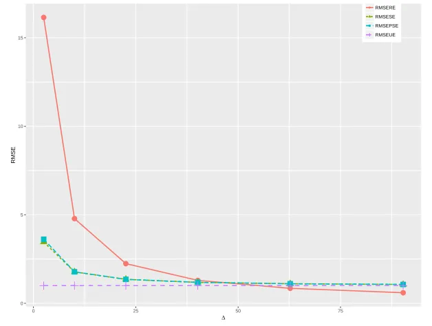
8.3 RMSE of UE, RE, SE, PSE versus ∆ (m= 2, T = 20) . . . 71

8.4 RMSE of UE, RE, SE, PSE versus ∆ (m= 2, T = 50) . . . 72

8.5 RMSE of UMLE, RMLE, SE, PSE versus ∆ (m= 3, T = 20) . . . . 72

8.6 RMSE of UMLE, RMLE, SE, PSE versus ∆ (m= 3, T = 50) . . . . 73

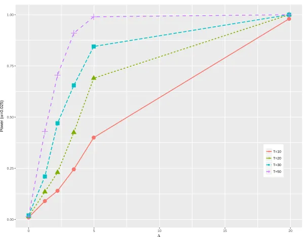
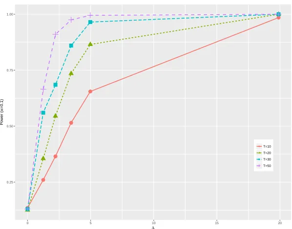
8.7 The empirical power of the test versus ∆ andT (m= 2) . . . 74

8.10 The empirical power of the test versus ∆ and T (m= 3) . . . 75

8.11 The empirical power of the test versus ∆ and T (m= 3) . . . 76

(13)

Chapter 1 Introduction and contributions

Nowadays, Ornstein-Uhlenbeck (O-U) processes are applied in different fields, such

as physical sciences (Lansky and Sacerdote (2001)) and biology (Rohlfset al.(2010)). The O-U process is also called the mean reverting process since the mean reverting

level is the component which has large effect on it. For the classical O-U processes,

the mean reverting level is constant. However, the classical O-U processes do not fit

well to data whose mean reverting level may change with the time. This is

partic-ularly the case for some phenomena which heavily depend on factors which change

with the time. For instance, government policy is one factor which affects the stock

price. Thus, if the government policies are changed in different time periods, the

mean reverting level of the stock price may change. As a result, the stock price is

changed. To overcome such a problem, Dehling et al. (2010) proposed a stochas-tic process which has a time-dependent periodic mean reverting function. This is

the so called generalized Ornstein-Uhlenbeck process. Further, to take into account

(14)

a closely related reference, we quote Chen et al. (2017) who proposed a method for detecting multiple change-points in generalized O-U process. In this thesis, we study

the inference problem in generalized O-U processes with multiple unknown

change-points where the drift parameter is suspected to satisfy some restrictions. We also

revisit the conditions for the main results in Chen et al. (2017) to hold. In particu-lar, we show that the results in Chen et al. (2017) hold without their Assumption 2. Nevertheless, the authors of the quoted paper omitted an important condition about

the initial value of the SDE for their main results to hold. In the subsequent section,

we highlight the main contribution of this thesis.

1.1 Main contributions

In this section, we present the main contributions of this thesis. Briefly, we generalize

the methods in Chen et al. (2017) as well as that in Nkurunziza and Zhang (2018). In particular, the proposed method generalizes the work of Chen et al. (2017) in five ways.

1. We consider a statistical model which incorporates the uncertain prior

knowl-edge.

2. We derive the unrestricted estimator (UE) and the restricted estimator (RE)

for the drift parameter.

3. For a known number of change-points, we derive the joint asymptotic normality

of the UE and the RE under the set of local alternative hypotheses.

4. We derive a test for testing the hypothesized restriction and we derive its

(15)

points.

5. We construct a class of shrinkage estimators (SEs) which includes as a special

case the UE, the RE and classical SEs. The proposed SEs are expected to be

robust with respect to the restriction.

The novelty of the derived results consists in the fact that the dimensions of the

proposed estimators are random variables. To overcome the difficulty due to the

randomness of the dimension, we establish two asymptotic results which are of interest

on their own.

1.2 Organization of the thesis

The remainder of this thesis is organized as follows. In Chapter 2, we introduce

the statistical model and assumptions. In Chapter 3, we study the joint asymptotic

normality of the UE and the RE in the case of known change-points. In Chapter

4, we study the joint asymptotic normality of the UE and the RE in the case of

unknown change-points. In Chapter 5, we present inference methods in the case of

unknown change-points and unknown number of change-points. In Chapter 6, we

construct a class of SEs and test the restriction. In Chapter 7, we compare the

relative performance between estimators. In Chapter 8, we present some simulation

results, and Chapter 9 gives some concluding remarks. Finally, for the convenience

(16)

Chapter 2 Statistical model and regularity

conditions

In this section, we present the statistical model of the generalized Ornstein-Uhlenbeck

process which is mainly studied in this thesis. Two assumptions are presented.

Un-der these assumptions, we Un-derive the log-likelihood function. In Chapter 3 and 4, we

use this log-likelihood function to derive the Maximum Likelihood Estimator (MLE) without restriction and with restriction.

The inference problem studied in this thesis was mainly inspired by the work in

Chen et al. (2017) where the authors proposed a method for detecting multiple change-points in generalized O-U processes. To give some other references about

inference problem in generalized O-U processes, we quote Dehling et al. (2010), Dehling et al. (2014), Nkurunziza and Zhang (2018). To introduce some notation, let {Wt;t ≥ 0} be a one-dimensional standard Brownian motion (Wiener process)

defined on some probability space (Ω,F, P) and let σ > 0. The change points are

(17)

τ0 = 0 and τm+1 = T to simplify the notation. Let > denote the transpose of a

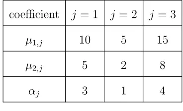
matrix, let θ = (θ>₁, . . . , θ_m>₊₁)> with θj = (µ1,j, . . . , µp,j, aj)> for τj−1 < t ≤ τj

where, for j = 1, . . . , m+ 1 and k = 1, . . . , p, µk,j is real value and aj > 0. Let

ϕ(t) = (ϕ1(t), ϕ2(t), . . . , ϕp(t)). Let I{.} be an indicator function, and let Ip be the

p-dimensional identity matrix. As in Chen et al. (2017), we consider the stochastic differential equation (SDE) given by

dXt =S(θ, t, Xt)dt+σdWt, 0≤t ≤T (2.1)

where the drift coefficient, S(θ, t, Xt), is as follows

S(θ, t, Xt) =

m+1

X

j=1

p X

k=1

µk,jϕk(t)−ajXt !

I{τj−1<t≤τj}. (2.2)

In the SDE given in (2.1) and (2.2), m represents the number of unknown

change-points (m≥1), while τ1, τ2, . . . , τm are the locations of change-points. In this thesis,

the parameter of interest is θ while m, τ1, τ2, . . ., τm are the unknown nuisance

pa-rameters.

Sometimes, there exists a prior knowledge, calledprior information, so that we might use both the non-sample information and the sample information to estimate the parameters. In this thesis, the prior information is considered as a form of a linear

constraint on θ for a given m, τ1, τ2, . . ., τm. Then, when τ1, τ2, . . ., τm and m are

known, the maximum likelihood estimator, which is derived based on linear

restric-tions, is called theRestricted Maximum Likelihood Estimator (RMLE). In particular, we consider the scenario where the target parameter may satisfy the restriction

H0 :Bθ =r (2.3)

(18)

to the hypothesis testing problem

H0 :Bθ =r vs H1 :Bθ 6=r. (2.4)

Particularly, if we choose r= 0 and

B =



        

Ip+1 −Ip+1 0 . . . 0 0

0 Ip+1 −Ip+1 . . . 0 0

..

. ... ... . .. ... ...

0 0 0 . . . Ip+1 −Ip+1



        

=B0,

the restriction in (2.3) corresponds to the case where there are no change points.

Thus, the testing problem in (2.4) includes as a special case testing the absence of

change points.

Assumption 1. The distribution of the initial value, X0, of the SDE in (2.1) does

not depend on the drift parameter θ. Further, X0 is independent of {Wt:t≥0} and

E[|X0| d

]<∞, for some d≥2.

Assumption 2. For anyT >0, the basis functions{ϕk(t), k= 1, ..., p}are

Riemann-integrable on [0, T] and satisfy

(1) Periodicity: ϕ(t+v) = ϕ(t) where v is the period in the data. (2) Orthogonality in L2_([0_{, v}_]1

vdλ):

Z v

0

ϕ(t)ϕ>(t)dt =vIP.

Remark 1. Assumption 2 corresponds to a similar assumption in Chen et al. (2017). Assumption 1 is not explicitly given in Chen et al. (2017), but their results require the Assumption 1 to hold. For example, if E[|X0|2] =∞, the relation (3.8) in Chen et al.

(2017) does not hold. Further, if the distribution ofX0 depends onθ, by Theorem 1.12

(19)

Since, for k= 1, ..., p, ϕk(t) is bounded on [0, T] and is periodic, this implies that

ϕk(t) is bounded on R+. Without loss of generality, as in Chen et al. (2017), we

assume that v = 1.

The following proposition shows that the SDE (2.5) admits a strong and unique

solution.

Proposition 2.1. The SDE

dXt=

m+1

X

j=1

p X

k=1

I{τj−1<t≤τj}dt+σdWt (2.5)

0≤t≤T admits a strong and unique solution that is L2_{-bounded on} _[0_{, T}_]_{, i.e.,}

sup

0≤t≤T

E[X2

t]<∞.

Proof. It suffices to check whether the coefficients of SDE satisfy both space-variable Lipschitz condition and the spatial growth condition. For more details, see the proof

of Proposition 3.2 in Chen et al. (2017).

Lemma 2.1. The solution of SDE in (2.5) has the explicit representation

Xt =

m+1

X

j=1

Xj(t)I(τj−1<t≤τj), Xj(t) =e

−ajt_X

0 +hj(t) +zj(t), (2.6)

where

hj(t) =e−ajt p X

k=1

µk,j

Z t

0

eajs_ϕ

k(s)ds, zj(t) =σe−ajt

Z t

0

eajs_dW

s. (2.7)

Further, sup

t≥0

E[|Xt|2]<∞.

The proof is given in Appendix B.

Note that process{Xt}{τj−1<t≤τj} is not stationary. Because of that we cannot apply

(20)

We define, for τj−1 < t≤τj, j = 1, ..., m+ 1,

˜

Xj(t) = ˜hj(t) + ˜zj(t) (2.8)

where

˜

hj(t) =e−ajt p X

k=1

µk,j

Z t

−∞

eajs_ϕ

k(s)ds, z˜j(t) = σe−ajt

Z t

−∞

eajs_d_B˜

s, (2.9)

where {B˜s}s∈_R denotes a bilateral Brownian motion. i.e.

˜

Bs=BsIR+(s) + ¯B−sIR−(s)

with {Bs}s≥0 and {B¯−s}s≥0 being two independent standard Brownian motions.

Let Σj be a (p+ 1)×(p+ 1) non-random matrix as, forj = 1, ..., m+ 1,

Σj = 

 

IP Λj

ΛT

j ωj





 (2.10)

where

Λj =−

Z 1

0

˜

hj(t)ϕ(t)dt, ωj =

Z 1

0

˜

h2_j(t)dt+ σ

2

2aj

,

with the function ˜hj(t) : [0,∞]→R

˜

hj(t) =e−ajt p X

k=1

µk,j

Z t

−∞

eajs_ϕ

k(s)ds.

Proposition 2.2. Suppose that Assumptions 1-2 hold, then, for k = 0,1, . . ., (1) E[ ˜Xj(t+k)] = ˜hj(t);

(2) Cov( ˜Xj(t),X˜j(t+k)) =e−ajk

σ2

2aj

.

The proof is given in Appendix B. From Proposition 2.2, we derive the following

(21)

Lemma 2.2. For t ∈ [0,1], for j = 1,2, . . . , m, the sequence of random variables

{X˜j(k+t)}k∈N0 is stationary and ergodic.

Remark 2. From Proposition 2.1, we have P

Z T

0

S2(θ, t, Xt)dt <∞

= 1, for all

0 < T < ∞ and elements θj of θ involved in S(θ, t, Xt) given by equation (2.1). In

passing, it should be noticed that this condition is given as a required assumption in Chen et al. (2017, Assumption 2). Thus, here we show that the results in Chen et al. (2017) hold without their Assumption 2.

This condition is useful in deriving the likelihood function of the SDE in (2.1).

Proposition 2.3. If Assumption 1-2 hold, then the log likelihood function is

logL(θ, Xt) =

1

σ2

m+1

X

j=1

θ>_j r˜(τj−1,τj)−

1 2σ2

m+1

X

j=1

θ>_j Q(τj−1,τj)θj (2.11)

where

˜

r(τj−1,τj) =

Z τj

τj−1

ϕ1(t)dXt, ...,

Z τj

τj−1

ϕp(t)dXt,−

Z τj

τj−1

XtdXt !>

(2.12)

and

Q(τj−1,τj) = 

      

Z τj

τj−1

ϕ2₁(t)dt . . .

Z τj

τj−1

ϕ1(t)ϕp(t)dt −

Z τj

τj−1

ϕ1Xtdt

..

. ... ... ...

−

Z τj

τj−1

ϕ1Xtdt . . . −

Z τj

τj−1

ϕpXtdt

Z τj

τj−1

X_t2dt



      

. (2.13)

The proof is given in Appendix B. The following proposition shows that the matrix

(22)

the UMLE for θ. To introduce some notation, let φ= (φ1, . . . , φm)>. Let

˜

R(φ, m) = (˜r(0,τ1), ...,r˜(τm,T)) >

, Q(φ, m) =



        

Q(0,τ1) 0 . . . 0

0 Q(τ1,τ2) . . . 0

..

. ... . .. ...

0 0 . . . Q(τm,T)



        

. (2.14)

Proposition 2.4. Suppose that Assumption 1-2 holds. Then, if

T ≥ 1

(φj−φj−1)

, Q(τj−1,τj) is positive definite for j = 1, . . . , m+ 1. Further, if

T ≥ 1

min

1≤j≤m+1(φj −φj−1)

, Q(φ, m) is a positive definite matrix.

The proof of this proposition is similar to that of Proposition 3.2 of Shen (2018, p. 32).

(23)

Chapter 3 Estimation in the case of known

change points

3.1 The unrestricted estimator

In this chapter, we assume that the change point τj = φjT is known, j = 1, ..., m.

Then, some preliminary results related to theMaximum Likelihood Estimator (MLE) of drift parameter are developed. In this chapter, all the estimation problems are

studied on the basis of the sample information. Hence, the derived MLE is called the

Unrestricted Maximum Likelihood estimator (UMLE). We also derive the asymptotic normality of the UMLE.

3.1.1 The UMLE

θ

ˆ

(

φ, m

)

The UMLE ˆθ(φ, m) is derived based on Proposition 2.3 along with the positive

(24)

By relation (2.11) in Proposition 2.3, we have

logL(θ, Xt) =

1

σ2θ

>_˜

R(φ, m)− 1

2σ2θ >

Q(φ, m)θ. (3.1)

Next, from Proposition 2.4, we derive the UMLE which is given in the following

lemma.

Lemma 3.1. Suppose that Assumptions 1-2 hold, and let R˜(φ, m)and Q(φ, m) be as defined in (2.14). Then the UMLE of θ is

ˆ

θ(φ, m) = Q−1(φ, m) ˜R(φ, m).

.

The proof is given in Appendix B. Let

R(φ, m) = (r(0,τ1), ..., r(τm,T)) >

(3.2)

and

r(a, b) =

Z b

a

ϕ1(t)dWt, ...,

Z b

a

ϕp(t)dWt,−

Z b

a

XtdWt !>

for 0 ≤ a < b ≤ T, and Q(φ, m) defined in (2.14). From Lemma 3.1, we derive

the following proposition which is useful in deriving the asymptotic normality of the

UMLE.

Proposition 3.1. Suppose that Assumptions 1-2 hold. The UMLE of θ can be rewritten as

ˆ

θ(φ, m) =θ+σQ−1(φ, m)R(φ, m). (3.3)

By Lemma 3.1, we can rewrite the UMLE of the drift parameter

ˆ

θ=Q−1(φ, m) ˜R(φ, m) = T Q−1(φ, m)1

T

˜

R(φ, m) = (1

TQ(φ, m))

−11

T

˜

(25)

Thus, in order to study the convergence of ˆθ(φ, m), we study first the convergence of

(1

TQ(φ, m))

−1_{. To introduce some notation, let} _−−−→P

T→∞ ,

d

−−−→

T→∞ ,

Lp

−−−→

T→∞ ,

a.s.

−−−→

T→∞ denote

convergence in probability, in distribution , inLp_{-space and almost surely respectively,}

as T tends to infinity.

Proposition 3.2. If Assumption 2 holds, then, for 0≤φj−1 < φj ≤1,

j = 1, ..., m+ 1, 1

T

Z φjT

φj−1T

ϕ(t)ϕ>(t)dt−−−→a.s.

T→∞ (φj−φj−1)IP.

Proposition 3.3. Suppose that Assumptions 1-2 hold. Then, 0 ≤ φj−1 < φj ≤ 1

where j = 1, ..., m+ 1,

1

T

Z φjT

φj−1T

Xtϕ(t)dt P

−−−→

T→∞ (φj −φj−1)

Z 1

0

˜

hj(t)ϕ(t)dt.

Proposition 3.4. Suppose that Assumptions 1-2 hold. Then, 0 ≤ φj−1 < φj ≤ 1,

j = 1, ..., m+ 1,

1

T

Z φjT

φj−1T

X_t2dt −−−→P

T→∞ (φj −φj−1)

"

Z 1

0

(˜hj(t))2dt+

σ2

2aj #

.

The proof is given in Appendix B. Let

Σ =



        

φ1Σ1 0 . . . 0

0 (φ2−φ1)Σ2 . . . 0

..

. ... . .. ...

0 0 . . . (1−φm)Σm+1



        

.

Proposition 3.5. Suppose that Assumption 2 holds. Then, Σj is a positive definite

(26)

The proof is given in Appendix B. By combining Propositions 3.2-3.4, we derive

the following proposition.

Proposition 3.6. If Assumptions 1-2 hold, then, for 0 ≤ φj−1 < φj ≤ 1, j =

1, ..., m+ 1, T Q−₍_τ1

j−1,τj) P

−−−→

T→∞

1

φj −φj−1

(Σj)−1. Further, T Q−1(φ, m) P

−−−→

T→∞ Σ

−1_.

The proof is given in Appendix B. It should be noticed that in Nkurunziza and

Fu (2018), we prove a stronger result. Indeed, we prove that the above convergences

hold almost surely.

3.1.2 Asymptotic normality of the UMLE

θ

ˆ

(

φ, m

)

In this subsection, we study the convergence of √1

TR(φ, m). Then, based on that

convergence, we establish the asymptotic normality of the UMLE ˆθ(φ, m).

The following proposition gives the limiting distribution of √1

TR(φ, m).

Proposition 3.7. Suppose that Assumptions 1-2 hold. Then,

1

√

TR(φ, m)

d

−−−→

T→∞ r

∗ _{∼ N}

(m+1)(p+1)(0,Σ).

The proof is given in Appendix B. From Proposition 3.7, we derive below a

proposition which gives the asymptotic normality of the UMLE. To simplify some

mathematical expressions, let ρT(φ, m) =

√

T(ˆθ(φ, m)−θ).

Proposition 3.8. Suppose that Assumptions 1-2 hold. Then, the UMLE ˆθ(φ, m) is asymptotically normal, i.e., ρT(φ, m)

d

−−−→

T→∞ ρ∼ N(m+1)(p+1)(0, σ

2_Σ−1₎_.

3.2 The restricted estimator

(27)

Proposition 3.9. Suppose that Assumptions 1-2 hold along with (2.3) and let

G=Q−1₍_{φ, m}₎_B>₍_BQ−1₍_{φ, m}₎_B>₎−1_{. Then, the RMLE of} _θ _is

˜

θ(φ, m) = ˆθ(φ, m)−G(Bθˆ(φ, m)−r). (3.5)

3.2.1 Asymptotic normality of the RMLE

θ

˜

(

φ, m

)

In this subsection, we study the asymptotic property of the RMLE ˜θ(φ, m) based on

the asymptotic normality of the UMLE ˆθ(φ, m). Based on Proposition 3.9, we have

√

T(˜θ(φ, m)−θ) = √T[Gr+ (I(m+1)(p+1)−GB)ˆθ(φ, m)−θ]

=√T(Gr−θ) +√T(I(m+1)(p+1)−GB)ˆθ(φ, m).

This gives

√

T(˜θ(φ, m)−θ) = (I(m+1)(p+1)−GB)

√

T(ˆθ(φ, m)−θ)−√T G(Bθ−r).

Now, we defineζT(φ, m) =

√

T(˜θ(φ, m)−θ). We have

ζT(φ, m) = (I(m+1)(p+1)−GB)

√

T(ˆθ(φ, m)−θ)−√T G(Bθ−r). (3.6)

Consider a continuous functiong(X) = XB>(BXB>)−1_where_X_{is a positive definite}

matrix. We have

g(T Q−1(φ, m)) =G=T Q−1(φ, m)B>(BT Q−1(φ, m)B>)−1.

By combining Proposition 3.6, and the continuous mapping theorem,

G−−−→P

T→∞ G

∗

(28)

and

I(m+1)(p+1)−GB P

−−−→

T→∞ I(m+1)(p+1)−G

∗

B. (3.7)

To study the asymptotic normality of the RMLE ˜θ(φ, m), we consider the following

set of local alternative restrictions,

Ha,T :Bθ−r =

r0

√

T, T >0 (3.8)

where r0 is a fixedq-column vector. Then,

√

T G(Bθ−r) = √T G√r0

T =Gr0

P

−−−→

T→∞ G

∗_r

0. (3.9)

Proposition 3.10. Suppose that Assumptions 1-2 hold along with the set of local alternatives in (3.8). Then RMLE ˜θ(φ, m) given in (3.5) is asymptotically normal, i.e., ζT(φ, m)

d

−−−→

T→∞ ζ ∼ N(m+1)(p+1) −G

∗

r0, σ2(Σ−1 −G∗BΣ−1)

.

3.3 Joint asymptotic normality of

θ

ˆ

(

φ, m

)

and

θ

˜

(

φ, m

)

In this section, we establish the joint asymptotic normality of UMLE ˆθ(φ, m) and

RMLE ˜θ(φ, m). This property is the foundation of developing a test for the testing

problem in (2.4) as well as its power. The established result is also useful in

construct-ing shrinkage estimators and their asymptotic efficiency. The followconstruct-ing proposition

presents the asymptotic property of

(ρ>_T(φ, m), ζ_T>(φ, m))> =√T(ˆθ(φ, m)−θ)>,(˜θ(φ, m)−θ)>

>

.

(29)

alternatives in (3.8). Then, (ρ>_T(φ, m), ζ_T>(φ, m))>−−−→d

T→∞ (ρ

>_{, ζ}>₎>_{, where}    ρ ζ  

∼ N2(m+1)(p+1)

      0

−G∗_r 0   , σ 2   

Σ−1 Σ−1−G∗BΣ−1

Σ−1−G∗BΣ−1 Σ−1−G∗BΣ−1

     .

Proof. We observe that



 

√

T(ˆθ(φ, m)−θ)

√

T(˜θ(φ, m)−θ)

  =    √

T(ˆθ(φ, m)−θ)

(I(m+1)(p+1)−GB)

√

T(ˆθ(φ, m)−θ)−√T G(Bθ−r)

   =   

I(m+1)(p+1)

I(m+1)(p+1)−GB 

 

√

T(ˆθ(φ, m)−θ) +

   0 −Gr0   .

From (3.7), we get



 

I(m+1)(p+1)

I(m+1)(p+1)−GB    P −−−→ T→∞   

I(m+1)(p+1)

I(m+1)(p+1)−G∗B 



 (3.10)

where all the elements in (3.10) are non-random. Similarly, by (3.9), we have

   0 −Gr0    P −−−→ T→∞    0

−G∗_r 0





. (3.11)

Then, by combining Proposition 3.8 and the relations (3.10) and (3.11) along with

Slutsky’s Theorem,



 

√

T(ˆθ(φ, m)−θ)

√

T(˜θ(φ, m)−θ)

   d −−−→ T→∞   

I(m+1)(p+1)

I(m+1)(p+1)−G∗B   ρ+    0

−G∗_r 0   =    ρ ζ   .

Then, by Proposition A.2 in Appendix A, (ρ>_T(φ, m), ζ_T>(φ, m))> −−−→d

T→∞ (ρ

>_{, ζ}>₎>_with

   ρ ζ  

∼ N2(m+1)(p+1)

       0

−G∗_r 0   , σ 2   

I(m+1)(p+1)

I(m+1)(p+1)−G∗B   Σ −1   

I(m+1)(p+1)

(30)

Note that

σ2



 

I(m+1)(p+1)

I(m+1)(p+1)−G∗B   Σ −1   

I(m+1)(p+1)

I(m+1)(p+1)−G∗B 

  >

=σ2



 

Σ−1 Σ−1−Σ−1B>G∗>

Σ−1−G∗BΣ−1 Σ−1−Σ−1B>G∗>−G∗BΣ−1+G∗BΣ−1B>G∗>





.

By the proof of Proposition 3.10, we know

G∗BΣ−1B>G∗> = Σ−1B>G∗>, (3.12)

and, since G∗ = Σ−1B>(BΣ−1B>)−1,

Σ−1B>G∗> = Σ−1B>(BΣ−1B>)−1BΣ−1 =G∗BΣ−1. (3.13)

Therefore, by (3.12) and (3.13),

σ2



 

I(m+1)(p+1)

I(m+1)(p+1)−G∗B   Σ −1   

I(m+1)(p+1)

I(m+1)(p+1)−G∗B 

  >

=σ2



 

Σ−1 _Σ−1₋_G∗_B_Σ−1

Σ−1₋_G∗_B_Σ−1 _Σ−1₋_G∗_B_Σ−1 



.

Finally, we have (ρ>_T(φ, m), ζ_T>(φ, m))> −−−→d

T→∞ (ρ

>_{, ζ}>₎>_, _where

   ρ ζ  

∼ N2(m+1)(p+1)

      0

−G∗_r 0   , σ 2   

Σ−1 _Σ−1₋_G∗_B_Σ−1

Σ−1₋_G∗_B_Σ−1 _Σ−1₋_G∗_B_Σ−1      .

This completes the proof.

Now, we define ξT(φ, m) =

√

T(ˆθ(φ, m)−θ˜(φ, m)). Next, we study the asymptotic

distribution of (ρ>_T(φ, m), ξ_T>(φ, m))> =√T

(ˆθ(φ, m)−θ)>,(ˆθ(φ, m)−θ˜(φ, m))>

>

(31)

Proposition 3.12. Suppose that Assumptions 1-2 hold along with the set of local alternatives in (3.8). Then, (ρ>_T(φ, m), ξ_T>(φ, m))> −−−→d

T→∞ (ρ

>_{, ξ}>₎>_{, where}    ρ ξ  

∼ N2(m+1)(p+1)

      0

G∗r0   , σ 2   

Σ−1 _G∗_B_Σ−1

G∗BΣ−1 _G∗_B_Σ−1      .

Proof. We have



 

√

T(ˆθ(φ, m)−θ)

√

T(ˆθ(φ, m)−θ˜(φ, m))

  =   

I(m+1)(p+1) 0

I(m+1)(p+1) −I(m+1)(p+1)       √

T(ˆθ(φ, m)−θ)

√

T(˜θ(φ, m)−θ)

  . We know   

I(m+1)(p+1) 0

I(m+1)(p+1) −I(m+1)(p+1)    P −−−→ T→∞   

I(m+1)(p+1) 0

I(m+1)(p+1) −I(m+1)(p+1) 



,

and, by Proposition 3.11 and Slutsky’s Theorem, we have



 

√

T(ˆθ(φ, m)−θ)

√

  =   

I(m+1)(p+1) 0

I(m+1)(p+1) −I(m+1)(p+1)       √

T(ˆθ(φ, m)−θ)

√

T(˜θ(φ, m)−θ)

   d −−−→ T→∞   

I(m+1)(p+1) 0

I(m+1)(p+1) −I(m+1)(p+1)       ρ ζ   =    ρ ξ   . Note that   

I(m+1)(p+1) 0

I(m+1)(p+1) −I(m+1)(p+1)       0

−G∗_r 0   =    0

G∗r0 



(32)

and



 

I(m+1)(p+1) 0

I(m+1)(p+1) −I(m+1)(p+1)   σ 2   

Σ−1 _Σ−1₋_G∗_B_Σ−1

Σ−1 ₋_G∗_B_Σ−1 _Σ−1₋_G∗_B_Σ−1    ×   

I(m+1)(p+1) I(m+1)(p+1)

0 −I(m+1)(p+1) 

 

=σ2



 

Σ−1 _Σ−1₋_G∗_B_Σ−1

G∗BΣ−1 0

     

I(m+1)(p+1) I(m+1)(p+1)

0 −I(m+1)(p+1) 

 

=σ2



 

Σ−1 G∗BΣ−1

G∗BΣ−1 G∗BΣ−1





.

Therefore, by Proposition A.2 in Appendix A,



 

ρT(φ, m)

ξT(φ, m)    d −−−→ T→∞    ρ ξ  

∼ N2(m+1)(p+1)

      0

G∗r0   , σ 2   

Σ−1 _G∗_B_Σ−1

G∗BΣ−1 _G∗_B_Σ−1      ,

this completes the proof.

From Proposition 3.12, we have following corollary.

Corollary 3.1. Suppose that Assumptions 1-2 hold along with the set of local alter-natives in (3.8). Then, ξT(φ, m)

d

−−−→

T→∞ ξ∼ N(m+1)(p+1)(G

∗_r

0, σ2G∗BΣ−1).

The proof follows directly from Proposition 3.12. Further, we study the asymptotic

property of (ζ_T>(φ, m), ξ_T>(φ, m))>=√T(˜θ(φ, m)−θ)>,(ˆθ(φ, m)−θ˜(φ, m))>

>

.

Proposition 3.13. Suppose that Assumptions 1-2 hold along with the set of local alternatives in (3.8). Then, (ζ_T>(φ, m), ξ_T>(φ, m))> −−−→d

T→∞ (ζ

>_{, ξ}>₎>_{, where}    ζ ξ  

∼ N2(m+1)(p+1)

     

−G∗_r 0

G∗r0   , σ 2   

Σ−1 −G∗BΣ−1 0

0 G∗BΣ−1

(33)

Proof. We observe that



 

√

T(˜θ(φ, m)−θ)

√

  =   

0 I(m+1)(p+1)

I(m+1)(p+1) −I(m+1)(p+1)       √

T(ˆθ(φ, m)−θ)

√

T(˜θ(φ, m)−θ)

  . (3.14) Further,   

0 I(m+1)(p+1)

I(m+1)(p+1) −I(m+1)(p+1)    P −−−→ T→∞   

0 I(m+1)(p+1)

I(m+1)(p+1) −I(m+1)(p+1)   , and   

ρT(φ, m)

ζT(φ, m)    d −−−→ T→∞    ρ ζ   

∼ N2(m+1)(p+1)       0

−G∗_r 0   , σ 2   

Σ−1 _Σ−1₋_G∗_B_Σ−1

Σ−1₋_G∗_B_Σ−1 _Σ−1₋_G∗_B_Σ−1 

 





. (3.15)

Then, by combining (3.14) and (3.15) and Slutsky’s Theorem, we get



 

ζT(φ, m)

ξT(φ, m)    d −−−→ T→∞   

0 I(m+1)(p+1)

I(m+1)(p+1) −I(m+1)(p+1)       ρ ζ   =    ζ ξ   . Note that   

0 I(m+1)(p+1)

I(m+1)(p+1) −I(m+1)(p+1)       0

−G∗_r 0   =   

−G∗_r 0

G∗r0 



(34)

and



 

0 I(m+1)(p+1)

I(m+1)(p+1) −I(m+1)(p+1) 



σ

2 

 

Σ−1 _Σ−1₋_G∗_B_Σ−1

Σ−1₋_G∗_B_Σ−1 _Σ−1₋_G∗_B_Σ−1 

 

×



 

0 I(m+1)(p+1)

I(m+1)(p+1) −I(m+1)(p+1) 

 

=σ2



 

Σ−1₋_G∗_B_Σ−1 _Σ−1₋_G∗_B_Σ−1

G∗BΣ−1 ₀



 



 

0 I(m+1)(p+1)

I(m+1)(p+1) −I(m+1)(p+1) 

 

=σ2



 

Σ−1−G∗BΣ−1 0

0 G∗BΣ−1





.

Therefore, by Proposition A.2 in Appendix A, (ζ_T>(φ, m), ξ_T>(φ, m))> −−−→d

T→∞ (ζ

>_{, ξ}>₎>

with



 

ζ

ξ





∼ N2(m+1)(p+1)



 



 

−G∗_r 0

G∗r0 



, σ

2 

 

Σ−1 −G∗BΣ−1 0

0 G∗BΣ−1



 





.

(35)

Chapter 4 Estimation in the case of unknown

change points

4.1 The unrestricted estimator

In the previous chapter, the locations of change-points, τ = (τ1, . . . , τm)>, and the

number of change points, m, are assumed to be known. Nevertheless, in practice,

the change points are also unknown. Thus, the change points have to be estimated

from the data. In this chapter, we assume that the number of change points, m, is

known but the locations of change points are unknown. We show that the asymptotic

property, in the case of known change points, holds when we replace change points

by their consistent estimators. Let ˆφj be a consistent estimator of the parameter φj,

j = 1, ..., m, and for convenience, let ˆφ0 = 0 and ˆφm+1 = 1. Let ˆφ = ( ˆφ1,φˆ2, . . . ,φˆm)>.

First, for estimating the locations of change points, we recall the least sum of squared

(36)

∆t = ti+1 −ti, are exactly the same for i = 0, ..., n−1. Moreover, we define Yi =

Xti+1−Xti and zi = (ϕ1(ti), ..., ϕp(ti),−Xti)∆t.

The exact value of the drift parameters θ may be different with the value of their

MLE because of the uncertain location of estimated change points. For instance, if

ˆ

τj > τj, then for all ti ∈ (τj,τˆj], it is obvious that the corresponding true value of

the drift parameters is θ(j+1)_{. However, in the same condition, the MLE of the drift}

parameters is ˆθ(j) _{for all} _t

i ∈ (τj,τˆj]. Therefore, we let θi =

Pm+1

j=1 θjI{τj−1<ti≤τj} be

the true value of the drift parameter at ti. Also, ˆθi =

Pm+1

j=1 θˆjI{ˆτj−1<ti≤τˆj} , where

ˆ

θj = Q−_(ˆ_τ1_j₋₁_,_ˆ_τ_j₎r˜(ˆτj−1,τˆj) for j = 1, ..., m+ 1, is set up to be the MLE of the drift

parameters at ti. By the Euler-Maruyama discretisation method, we have

Yi =ziθi+i, i= 1, ..., n (4.1)

wherei is the error termσ

√

∆tωi, andωiis theith independent draw from a standard

normal variable. From (4.1), the estimators for the m change points, τ, are given by

ˆ

τ = arg min

τ SSE([0, T], τ,

ˆ

θ(τ)) (4.2)

where

SSE([0, T], τ,θˆ(τ)) = X

ti∈[0,T]

(Yi−ziθˆi)T(Yi−ziθˆi) (4.3)

Assumption 3. For every j = 1, ..., m, there exists an L0 > 0 such that for all

L > L0 the minimum eigenvalues of

1

L

X

ti∈(τj,τj+L]

z_iTzi and of

1

L

X

ti∈(τj−L,τj]

z_iTzi as

well as their respective continuous-time versions 1

LQ(τj,τj+L) and

1

LQ(τj−L,τj), are all

bounded away from 0.

Remark 3. For the estimators of φj, we can directly obtain φˆj =

ˆ

τj

T,

(37)

B. Clearly, the estimator φˆj is FT-measurable and φˆj ∈ [0,1] for j = 1, ..., m+ 1.

Further, there exists δ0 >0 such that φˆj −φj =OP(T−δ0) for j = 1, ..., m.

We introduce another method to estimate the locations of the change points. This

is based on the Maximum log-likelihood. By Theorem 7.6 of Lipster and Shiryaev

(2001), the log-likelihood function is given by

logL(τ, θ) = 1

σ2

Z T

0

S(θ, t, Xt)dXt−

1 2σ2

Z T

0

S2(θ, t, Xt)dt,

where τ = (τ1, τ2, . . . , τm). Note that, by (B.16),

1

σ2

Z T

0

S(θ, t, Xt)dXt=

1 σ2 Z T 0 m+1 X j=1 p X k=1

I{τj−1<t≤τj}dXt

= 1 σ2 m+1 X j=1 Z T 0 p X k=1

I{τj−1<t≤τj}dXt.

This gives

1

σ2

Z T

0

S(θ, t, Xt)dXt=

1

σ2

m+1

X

j=1

Z τj

τj−1

p X

k=1

dXt.

Further, by the proof of Proposition 2.3,

1 2σ2

Z T

0

S2(θ, t, Xt)dt =

1 2σ2

Z T

0

"_m₊₁ X

j=1

p X

k=1

I{τj−1<t≤τj}

#2

dt

= 1

2σ2

Z T 0 m+1 X j=1 p X k=1

µk,jϕk(t)−ajXt

!2

I{τj−1<t≤τj}dt

= 1

2σ2

m+1 X j=1 Z T 0 p X k=1

µk,jϕk(t)−ajXt

!2

I{τj−1<t≤τj}dt.

This gives

1 2σ2

Z T

0

S2(θ, t, Xt)dt=

1 2σ2

m+1

X

j=1

Z τj

τj−1

p X

k=1

µk,jϕk(t)−ajXt

!2

(38)

Therefore, for the change points τ1, . . . , τm, the log-likelihood function for SDE (2.1)

is given by

logL(τ, θ) = 1

σ2

m+1

X

j=1

Z τj

τj−1

S(θj, t, Xt)dXt−

1 2σ2

m+1

X

j=1

Z τj

τj−1

S(θj, t, Xt)2dt (4.4)

where S(θj, t, Xt) = p X

k=1

µk,jϕk(t)−ajXt. From (4.4), when the number of change

point, m, is known, the estimator of τ is

ˆ

τ = arg max

τ logL(τ,

ˆ

θ(τ)) (4.5)

where ˆθ(τ) is the MLE ofθby using the given change pointsτ. Auger and Lawrence (1989)

introduced a numerical method to approximate the integrals inside the log-likelihood

function. In this case, we use this method to calculate logL(τ,θˆ(τ)) in (4.5). Divide

[0, T] into n parts, i.e. 0 = t∗₀ <· · ·< t∗_n = T with ∆∗_t = t∗_i₊₁−t∗_i. By the Riemann

sum, the log-likelihood function in (4.5) is approximated as

logL∗([0, T], τ,θˆ(τ)) = 1

σ2

m+1

X

j=1

X

t∗

i∈(τj−1,τj]

ˆ

θ>_j V(t∗_i)(Xt∗_i₊₁−Xt∗_i)

− 1

2σ2

m+1

X

j=1

X

t∗_i∈(τj−1,τj]

ˆ

θ>_j V(t∗_i)2∆∗_t (4.6)

where V(t) = (ϕ1(t), . . . , ϕp(t),−Xt)>. Then, the estimator of τ is given by

ˆ

τ = arg max

τ logL

∗

([0, T], τ,θˆ(τ)). (4.7)

For convenience, let ˆφ0 = 0 and ˆφm+1 = 1. In order to study the asymptotic properties

of the estimators of θ, we derive first the following preliminary results.

Lemma 4.1. Let {Yt, t ≥ 0} be a stochastic process {Ft, t ≥ 0}-adapted and L2

-bounded. Suppose that φˆj and φˆj−1 are FT-measurable and consistent estimators for

φj and φj−1 respectively, j = 1, ..., m+ 1, and 0≤φˆ1 < ... <φˆm ≤1 a.s.. Then,

1

T

Z φˆjT

ˆ

φj−1T

Ytdt−

1

T

Z φjT

φj−1T

Ytdt

L1

−−−→

(39)

Lemma 4.2. Let {Yt, t ≥ 0} be a Rp-valued deterministic and bounded function.

Suppose that φˆj and φˆj−1 are FT-measurable and consistent estimators for φj and

φj−1 respectively, j = 1, ..., m+ 1, and 0≤φˆ1 < ... <φˆm≤1 a.s.. Then,

1

√ T

Z φˆjT

ˆ

φj−1T

YtdWt−

1

√ T

Z φjT

φj−1T

YtdWt

L2

−−−→

T→∞ 0.

The proof is given in Appendix B. By using Lemma 4.1, we establish

Proposi-tions 4.1 and 4.2.

Proposition 4.1. If Assumptions 1-3 hold, then,0≤φj−1 < φj ≤1, j = 1, ..., m+ 1,

1

T

Z φˆjT

ˆ

φj−1T

ϕ(t)ϕ>(t)dt −−−→P

T→∞ (φj −φj−1)IP.

Proposition 4.2. Suppose that Assumptions 1-3 hold. Then, 0 ≤ φj−1 < φj ≤ 1,

j = 1, ..., m+ 1, (i) 1

T

Z φˆjT

ˆ

φj−1T

Xtϕ(t)dt−

1

T

Z φˆjT

ˆ

φj−1T

˜

Xtϕ(t)dt P

−−−→

T→∞ 0;

(ii) 1

T

Z φˆjT

ˆ

φj−1T

X_t2dt− 1 T

Z φˆjT

ˆ

φj−1T

˜

T→∞ 0.

The proof is given in Appendix B. By using Proposition 4.2, we derive

Proposi-tions 4.3 and 4.4.

Proposition 4.3. Suppose that Assumptions 1-3 hold. Then, for0≤φj−1 < φj ≤1,

j = 1, ..., m+ 1, 1

T

Z φˆjT

ˆ

φj−1T

Xtϕ(t)dt P

−−−→

T→∞ (φj−φj−1)

Z 1

0

˜

(40)

Proof. We have 1

T

Z φˆjT

ˆ

φj−1T

Xtϕ(t)dt =

1

T

Z φˆjT

ˆ

φj−1T

Xtϕ(t)dt−

1

T

Z φˆjT

ˆ

φj−1T

˜

Xtϕ(t)dt !

+ 1

T

Z φˆjT

ˆ

φj−1T

˜

Xtϕ(t)dt−

1

T

Z φjT

φj−1T

˜

Xtϕ(t)dt !

+ 1

T

Z φjT

φj−1T

˜

Xtϕ(t)dt−

1

T

Z φjT

φj−1T

Xtϕ(t)dt !

+ 1

T

Z φjT

φj−1T

Xtϕ(t)dt.

By Proposition 4.2

1

T

Z φˆjT

ˆ

φj−1T

Xtϕ(t)dt−

1

T

Z φˆjT

ˆ

φj−1T

˜

Xtϕ(t)dt P

−−−→

T→∞ 0. (4.8)

By Lemma 4.1,

1

T

Z φˆjT

ˆ

φj−1T

˜

Xtϕ(t)dt−

1

T

Z φjT

φj−1T

˜

Xtϕ(t)dt

L1

−−−→

T→∞ 0,

which implies that

1

T

Z φˆjT

ˆ

φj−1T

˜

Xtϕ(t)dt−

1

T

Z φjT

φj−1T

˜

Xtϕ(t)dt P

−−−→

T→∞ 0. (4.9)

As in the proof of Proposition 3.3, we have

1

T

Z φjT

φj−1T

˜

Xtϕ(t)dt−

1

T

Z φjT

φj−1T

Xtϕ(t)dt P

−−−→

T→∞ 0. (4.10)

By Proposition 3.3,

1

T

Z φjT

φj−1T

Xtϕ(t)dt P

−−−→

T→∞ (φj −φj−1)

Z 1

0

˜

hj(t)ϕ(t)dt. (4.11)

Finally, combining (4.8), (4.9), (4.10) and (4.11),

1

T

Z φˆjT

ˆ

φj−1T

Xtϕ(t)dt P

−−−→

T→∞ (φj −φj−1)

Z 1

0

˜

hj(t)ϕ(t)dt,

(41)

j = 1, ..., m+ 1, 1

T

Z φˆjT

ˆ

φj−1T

T→∞ (φj −φj−1)

"

Z 1

0

(˜hj(t))2dt+

σ2

2aj #

.

Proof. We have 1

T

Z φˆjT

ˆ

φj−1T

X_t2dt = 1

T

Z φˆjT

ˆ

φj−1T

X_t2dt− 1 T

Z φˆjT

ˆ

φj−1T

˜

X_t2dt

!

+ 1

T

Z φˆjT

ˆ

φj−1T

˜

X_t2dt− 1 T

Z φjT

φj−1T

˜

X_t2dt

!

+ 1

T

Z φjT

φj−1T

˜

X_t2dt− 1 T

Z φjT

φj−1T

X_t2dt

!

+ 1

T

Z φjT

φj−1T

X_t2dt.

By Proposition 4.2

1

T

Z φˆjT

ˆ

φj−1T

X_t2dt− 1 T

Z φˆjT

ˆ

φj−1T

˜

X_t2dt−−−→P

T→∞ 0. (4.12)

By Lemma 4.1,

1

T

Z φˆjT

ˆ

φj−1T

˜

X_t2dt− 1 T

Z φjT

φj−1T

˜

X_t2dt−−−→L1

T→∞ 0,

which implies that

1

T

Z φˆjT

ˆ

φj−1T

˜

X_t2dt− 1 T

Z φjT

φj−1T

˜

X_t2dt−−−→P

T→∞ 0. (4.13)

As in the proof of Proposition 3.4, we have

1

T

Z φjT

φj−1T

˜

X_t2dt− 1 T

Z φjT

φj−1T

X_t2dt−−−→P

T→∞ 0. (4.14)

By Proposition 3.4,

1

T

Z φjT

φj−1T

T→∞ (φj −φj−1)

"

Z 1

0

(˜hj(t))2dt+

σ2

2aj #

. (4.15)

Finally, combining (4.12), (4.13), (4.14) and (4.15),

1

T

Z φˆjT

ˆ

φj−1T

T→∞ (φj −φj−1)

"

Z 1

0

(˜hj(t))2dt+

σ2

2aj #

(42)

By combining Proposition 4.1, Proposition 4.3 and Proposition 4.4, we derive the

following propositions which give the same results as in Proposition 3.6 in case the

change points φj and φj−1 are replaced by their consistent estimators ˆφj and ˆφj−1

respectively.

First, we define

Q(ˆτj−1,ˆτj) =        

Z τˆj

ˆ

τj−1

ϕ2₁(t)dt . . .

Z τˆj

ˆ

τj−1

ϕ1(t)ϕp(t)dt − Z τˆj

ˆ

τj−1

ϕ1Xtdt

..

. ... ... ...

−

Z τˆj

ˆ

τj−1

ϕ1Xtdt . . . − Z τˆj

ˆ

τj−1

ϕpXtdt

Z τˆj

ˆ

τj−1

X_t2dt

        (4.16)

where ˆτj = ˆφjT, ˆτj−1 = ˆφj−1T for j = 1, ..., m+ 1.

j = 1, ..., m+ 1, T Q−_(ˆ_τ1

j−1,τˆj) P

−−−→

T→∞

1

φj−φj−1

(Σj)−1.

Proof. By Proposition 4.1, Proposition 4.3 and Proposition 4.4, we have 1

TQ(ˆτj−1,τˆj) P

−−−→

T→∞ (φj −φj−1)Σj, j = 1, ..., m+ 1.

By combining Propositions 2.4, 3.5, and the continuous mapping theorem, we get

T Q−_(ˆ_τ1

j−1,ˆτj) P

−−−→

T→∞

1

φj −φj−1

(Σj)−1. This completes the proof.

Now, we define

Q( ˆφ, m) =

         

Q(0,τˆ1) 0 . . . 0

0 Q(ˆτ1,τˆ2) . . . 0

..

. ... . .. ...

0 0 . . . Q(ˆτm,T)

(43)

Proposition 4.6. Suppose Assumptions 1-3 hold. Then, for 0 ≤ φj−1 < φj ≤ 1,

j = 1, ..., m+ 1, T Q−1( ˆφ, m)−−−→P

T→∞ Σ

−1_.

Next, we derive some results which generalize Proposition 3.7 and Proposition 3.8.

The results show that similar propositions hold with the change-points replaced by

their consistent estimators. Let ˆτj = ˆφjT, j = 1, ..., m+ 1, and let

R( ˆφ, m) = (r(0,τˆ1), ..., r(ˆτm,T)) >

, (4.18)

r(a, b) =

Z b

a

ϕ1(t)dWt, ...,

Z b

a

ϕp(t)dWt,−

Z b

a

XtdWt !>

,

for 0≤a < b≤T.

4.1.1 Asmptotic normality of the UE

θ

ˆ

( ˆ

φ, m

)

In deriving the asymptotic normality of the UE, we use the following lemma.

Lemma 4.3. Let {Yt, t≥0} be a solution of SDE

dYt =

m+1

X

k=1

f(µk, Yt)I{τj−1<t≤τj}dt+σdWt, 0≤t≤T (4.19)

where f(θ, x) is a real-valued function such that the processes {Yt, t ≥0} and

{f(θ, Yt), t ≥ 0} are L2-bounded. Suppose that φˆj and φˆj−1 are FT-measurable and

consistent estimators for φj and φj−1 respectively, j = 1, ..., m+ 1, and

(44)

max

1≤j≤m(|

ˆ

φj −φj|) =OP(T−δ0). Then, for 0≤φj−1 < φj ≤1,

j = 1, . . . , m+ 1, √1 T

Z φˆjT

ˆ

φj−1T

YtdWt−

1

√ T

Z φjT

φj−1T

YtdWt P

−−−→

T→∞ 0.

The proof is given in Appendix B. Lemma 4.3 yields Lemma 3.3 in Nkurunziza

and Zhang (2018) for whichm = 1.

j = 1, ..., m+ 1, √1 T

R( ˆφ, m)−R(φ, m)

_P

−−−→

T→∞ 0, whereR( ˆφ, m)is defined in (4.18)

and R(φ, m) is defined in (3.2).

The proof is given in Appendix B. By using Proposition 4.7, we derive the following

proposition which shows the limiting distribution of √1

TR( ˆφ, m).

Proposition 4.8. If the conditions in Proposition 4.7 hold, then, for

0≤φj−1 < φj ≤1, j = 1, ..., m+ 1,

1

√

TR( ˆφ, m)

d

−−−→

T→∞ r

∗ _{∼ N}

(m+1)(p+1)(0,Σ).

Proof. By Proposition 3.7 and Proposition 4.7, we have 1

√

TR(φ, m)

d

−−−→

T→∞ r

∗ _{∼ N}

(m+1)(p+1)(0,Σ)

and

1

√ T

R( ˆφ, m)−R(φ, m)−−−→P

T→∞ 0.

Hence, by Slutsky’s Theorem,

1

√

TR( ˆφ, m) =

1

√ T

R( ˆφ, m)−R(φ, m)+√1

TR(φ, m)

d

−−−→

T→∞ r

∗ _∼

N(m+1)(p+1)(0,Σ).

This completes the proof.

Now, let ˆτj = ˆφjT, j = 1, ..., m+ 1, and

˜

R( ˆφ, m) = (˜r(0,ˆτ1), ...,(˜r(ˆτm,T)) >

(45)

˜

r(a, b) =

Z b

a

ϕ1(t)dXt, ...,

Z b

a

ϕp(t)dXt,−

Z b

a

XtdXt !>

,

for 0≤a < b≤T.

Further, let ˆθ( ˆφ, m) = Q−1( ˆφ, m) ˜R( ˆφ, m) be the plug-in estimator whereQ( ˆφ, m) and

˜

R( ˆφ, m) are defined in (4.17) and (4.20). Now, we defineρT( ˆφ, m) =

√

T(ˆθ( ˆφ, m)−θ).

By combining Propositions 4.6 and 4.8, we derive the asymptotic normality of UE

ˆ

θ( ˆφ, m) in the following proposition.

Corollary 4.1. Suppose that the conditions in Proposition 4.7 hold. Then,

ρT( ˆφ, m) d

−−−→

T→∞ ρ∼ N(m+1)(p+1)(0, σ

2_Σ−1₎_.

4.2 The restricted estimator

In the previous chapter, we studied the asymptotic property of the Restricted Es-timator (RE) in context of known multiple change points. In this section, we give the Restricted Estimator (RE) in context of unknown multiple change-points. The estimator of the rate of change point ˆφj, which is consistent, will be involved instead

of the known rate of change point φj, j = 1, ..., m.

Proposition 4.9. Suppose that Assumptions 1-3 hold along with (2.3) and let

J =Q−1_{( ˆ}_{φ, m}₎_B>₍_BQ−1_{( ˆ}_{φ, m}₎_B>₎−1_{. Then, the} _RE _of _θ _is

˜

θ( ˆφ, m) = ˆθ( ˆφ, m)−J(Bθˆ( ˆφ, m)−r). (4.21)

This proof follows from the similar steps of the proof of Proposition 3.9. Since we

consider the case of unknown change points, we just replace ˜R(φ, m) andQ(φ, m) by

(46)

4.2.1 Asymptotic normality of the RE

θ

˜

( ˆ

φ, m

)

In this section, we derive the asymptotic normality of the RE ˜θ( ˆφ, m) based on the

asymptotic normality of the Unrestricted Estimator (UE) ˆθ( ˆφ, m). We show that the RE ˜θ( ˆφ, m) has the same limiting distribution as the RMLE ˜θ(φ, m). The established

result is similar to that in Perron and Qu (2006), Chen and Nkurunziza (2015),

Nkurunziza and Zhang (2018) among others.

Based on Proposition 4.9, we have

√

T(˜θ( ˆφ, m)−θ) =√T[J r+ (I(m+1)(p+1)−J B)ˆθ( ˆφ, m)−θ]

=√T(J r−θ) +√T(I(m+1)(p+1)−J B)ˆθ( ˆφ, m),

this gives

√

T(˜θ( ˆφ, m)−θ) = (I(m+1)(p+1)−J B)

√

T(ˆθ( ˆφ, m)−θ)−√T J(Bθ−r).

Now, we defineζT( ˆφ, m) =

√

T(˜θ( ˆφ, m)−θ). Then,

√

T(˜θ( ˆφ, m)−θ) = (I(m+1)(p+1)−J B)

√

T(ˆθ( ˆφ, m)−θ)−√T J(Bθ−r). (4.22)

Consider a continuous functiong(X) = XB>(BXB>)−1_where_X_{is a positive definite}

matrix. We have g(T Q−1_{( ˆ}_{φ, m}_{)) =}_J ₌_{T Q}−1_{( ˆ}_{φ, m}₎_B>₍_{BT Q}−1_{( ˆ}_{φ, m}₎_B>₎−1_.

By combining Proposition 4.6 and the continuous mapping theorem, we get

J =T Q−1( ˆφ, m)B>(BT Q−1( ˆφ, m)B>)−1 −−−→P

T→∞ Σ

−1

B>(BΣ−1B>)−1 =G∗,

and

I(m+1)(p+1)−J B P

−−−→

T→∞ I(m+1)(p+1)−G

∗

B. (4.23)

Under the set of local alternatives in (3.8), we have

√

T J(Bθ−r) =√T J√r0

T =J r0

P

−−−→

T→∞ G

∗

(47)

Corollary 4.2 which shows the asymptotic normality of the RE ˜θ( ˆφ, m) is given in the

next section.

4.3 Joint asymptotic normality of

θ

ˆ

( ˆ

φ, m

)

and

θ

˜

( ˆ

φ, m

)

In this section, we present the joint asymptotic normality of UE ˆθ( ˆφ, m) and RE

˜

θ( ˆφ, m). First, we study the asymptotic distribution of

(ρ>_T( ˆφ, m), ζ_T>( ˆφ, m))> =√T(ˆθ( ˆφ, m)−θ)>,(˜θ( ˆφ, m)−θ)>

>

.

Proposition 4.10. Suppose that Assumptions 1-3 hold along with the set of local alternatives in (3.8). Then, if r0 6= 0, (ρ>T( ˆφ, m), ζ

>

T( ˆφ, m))

> _−−−→d

T→∞ (ρ

>_{, ζ}>₎> _{and if}

r0 = 0, (ρ>T( ˆφ, m), ζ >

T( ˆφ, m))

> _−−−→d

T→∞ (ρ

>

0, ζ

>

0 )

>_{, where}    ρ ζ  

∼ N2(m+1)(p+1)

      0

−G∗_r 0   , σ 2   

Σ−1 Σ−1−G∗BΣ−1

Σ−1−G∗BΣ−1 Σ−1−G∗BΣ−1

     ,    ρ0 ζ0  

∼ N2(m+1)(p+1)

      0 0   , σ 2   

Σ−1 _Σ−1₋_G∗_B_Σ−1

Σ−1₋_G∗_B_Σ−1 _Σ−1₋_G∗_B_Σ−1      .

Proof. We can observe that



 

√

T(ˆθ( ˆφ, m)−θ)

√

T(˜θ( ˆφ, m)−θ)

  =    √

(I(m+1)(p+1)−J B)

√

T(ˆθ( ˆφ, m)−θ)−√T J(Bθ−r)

   =    √

(I(m+1)(p+1)−J B)

√

T(ˆθ( ˆφ, m)−θ)−J r0    =   

I(m+1)(p+1)

I(m+1)(p+1)−J B 

 

√

T(ˆθ( ˆφ, m)−θ) +



 

0

−J r0 



.

By (4.23), we know

(48)

Then,



 

I(m+1)(p+1)

I(m+1)(p+1)−J B    P −−−→ T→∞   

I(m+1)(p+1)

I(m+1)(p+1)−G∗B 



 (4.25)

where all the elements in (4.25) are non-random. Similarly, by (4.24), we have



 

0

−J r0    P −−−→ T→∞    0

−G∗_r 0





. (4.26)

By combining Corollary 4.1 and the relations (4.25), (4.26) along with Slutsky’s

Theorem,



 

ρT( ˆφ, m)

ζT( ˆφ, m)   =   

I(m+1)(p+1)

I(m+1)(p+1)−J B 

 

√

T(ˆθ( ˆφ, m)−θ) +



 

0

−J r0    d −−−→ T→∞   

I(m+1)(p+1)

I(m+1)(p+1)−G∗B   ρ+    0

−G∗_r 0   =    ρ ζ   

Then, by Proposition A.2 in Appendix A,



 

√

   d −−−→ T→∞    ρ ζ   

∼ N2(m+1)(p+1)        0

−G∗_r 0   , σ 2   

I(m+1)(p+1)

I(m+1)(p+1)−G∗B   Σ −1   

I(m+1)(p+1)

I(m+1)(p+1)−G∗B    >    .

Note that, from the proof of Proposition 3.11, we get



 

√

   d −−−→ T→∞    ρ ζ   

∼ N2(m+1)(p+1)       0

−G∗_r 0   , σ 2   

Σ−1 _Σ−1₋_G∗_B_Σ−1

Σ−1 ₋_G∗_B_Σ−1 _Σ−1₋_G∗_B_Σ−1      ,

Stein-rules and Testing in Generalized Mean Reverting Processes with Multiple Change-points

Scholarship at UWindsor

Scholarship at UWindsor

Stein-rules and Testing in Generalized Mean Reverting Processes

Stein-rules and Testing in Generalized Mean Reverting Processes

with Multiple Change-points

with Multiple Change-points

Stein-rules and Testing in Generalized Mean Reverting

Processes with Multiple Change-points

by

Kang Fu

A Thesis

Submitted to the Faculty of Graduate Studies

through the Department of Mathematics and Statistics

in Partial Fulfillment of the Requirements for

the Degree of Master of Science

at the University of Windsor

Windsor, Ontario, Canada

2018

Stein-rules and Testing in Generalized Mean Reverting

Processes with Multiple Change-points

by

Kang Fu

APPROVED BY:

D. Li

Department of Economics

M. Hlynka

Department of Mathematics and Statistics

S. Nkurunziza, Advisor

Department of Mathematics and Statistics

DECLARATION OF

CO-AUTHORSHIP / PREVIOUS

PUBLICATION

ABSTRACT

ACKNOWLEDGEMENTS

CONTENTS

LIST OF TABLES

LIST OF FIGURES

Chapter 1

Introduction and contributions

1.1

Main contributions

1.2

Organization of the thesis

Chapter 2

Statistical model and regularity

conditions

Chapter 3

Estimation in the case of known

change points

3.1

The unrestricted estimator

3.1.1

The UMLE

θ

ˆ

(

φ, m

)

3.1.2

Asymptotic normality of the UMLE

θ

ˆ

(

φ, m

)

3.2

The restricted estimator

3.2.1

Asymptotic normality of the RMLE

θ

˜

(

φ, m

)

3.3

Joint asymptotic normality of

θ

ˆ

(