The Effects of Individual Difference on Discrete Affective Picture Processing: An EEG Study.

(1)

ABSTRACT

LEE, JA YOUNG. The Effects of Individual Difference on Discrete Affective Stimuli Processing: An EEG Study. (Under the direction of Dr. Chang S. Nam.)

Engineering has been considered to be in the realm of rationality. In recent days, however, people started to think about the role of emotion in engineering, as they realize that emotion motivates our actions and decision-makings. According to the literature, emotions regulate various human behaviors (e.g., purchasing, risk-management, health-related habit, socializing) and it influences the engineering outcome of systems (e.g., trust, accuracy, efficiency, safety, satisfaction, etc.).

Bearing such significance of emotions in mind, the present study investigated how people process discrete affective picture stimuli, using electroencephalogram (EEG). Pictures in five different emotional categories (awe, excite, fear, disgust, and neutral) were presented to twenty male participants, and brain signals were measured during the image presentation. Furthermore, in order to examine how the emotion perception is affected by individual’s emotional intelligence (granularity), the tendency to represent emotional experience with precision and specificity, each participant’s emotional granularity was measured through an online survey. Event-related potential (ERP) and coherence of brain areas were then analyzed, subject to emotional granularity and discrete emotional categories.

(2)

(3)

The Effects of Individual Difference on Discrete Affective Stimuli Processing: An EEG Study

by Ja Young Lee

A thesis submitted to the Graduate Faculty of North Carolina State University

in partial fulfillment of the requirements for the Degree of

Master in Science

Industrial Engineering

Raleigh, North Carolina 2014

APPROVED BY:

__________________________________ Kristen Lindquist

__________________________________ Chang S. Nam

Chair of Advisory Committee

__________________________________ Yuan-Shin Lee

(4)

BIOGRAPHY

(5)

ACKNOWLEDGEMENTS

First and foremost, I would like to express my profound gratitude to Professor Chang S. Nam for his support, expert guidance, understanding and encouragement throughout my graduate studies. His incredible patience and wise counsel have given me strength to keep studying last two years.

Also, I am deeply grateful to my committee members. I wish to express my sincere thanks to Professor Kristen Lindquist of University of Chapel Hill for her careful and wise guidance of my project in emotion. Without her persistent help this thesis would not have been possible. In addition, I am grateful to Professor Ronald Endicott, who inspired me with Cognitive Science. I also thank to Professor Yuan-Shin Lee, who helped me to keep thinking critically in engineering perspective.

Thanks also go to my fellow graduate students at Human Factors and Ergonomics Area. Special thanks go to my friends who helped me throughout this academic exploration.

(6)

LIST OF TABLES

Table 1 Comparison of ‘emotion’ and ‘mood’ ... 4

Table 2 Comparison of emotion theories ... 6

Table 3 Determinants of affective processing ... 12

Table 4 ERP components and related cognitive processes ... 20

Table 5 Frequency bands and related cognitive functions ... 24

Table 6 Online surveys ... 27

Table 7 Intended emotions based on Mikels’ norm and the percentage of perceived emotion for each discrete intended emotion ... 30

Table 8 Channels and their functional locations ... 33

Table 9 Emotion words used to measure emotional granularity ... 38

Table 10 Participants' information ... 38

Table 11 Statistical analyses ... 44

Table 12 ANOVA: effect tests ... 44

Table 13 Effect of granularity on ERP amplitudes in each discrete emotion ... 52

(9)

LIST OF FIGURES

Figure 1 A simplified diagram of constructionist model ... 9!

Figure 2 Typical ERP waveform and components in response to affective visual stimuli ... 15!

Figure 3 Constructionist emotion model and corresponding ERP components ... 21!

Figure 4 Examples of IAPS images for each discrete emotion ... 28!

Figure 5 IAPS images on valence-arousal space ... 28!

Figure 6 Discrete emotion scores from Mikels’ norm (2005) ... 29!

Figure 7 Averaged complexity and dynamicity score of images in each emotional category31! Figure 8 Front panel of EEG recording program ... 32!

Figure 9 Montage ... 34!

Figure 10 Experiment procedure ... 40!

Figure 11 ERP components with three emotion categories ... 42!

Figure 12 Distribution of latencies and amplitudes of each ERP components ... 43!

Figure 13 Effect of discrete emotions on ERP components in low and high granular group 47! Figure 14 P2, N2 and EPN of two granularity groups ... 53!

Figure 15 The number of coherence reduction between high and low granularity group in beta band (α=0.01) ... 55!

Figure 16 Granularity effect on prefrontal-posterior coherence reduction, collapsed over emotions ... 55!

Figure 17 Revised mapping of constructionist model on ERP components ... 58!

(10)

LIST OF SYMBOLS AND ABBREVIATIONS

Abbreviations Intended Meaning

BA Brodmann’s Area

BAI Beck Anxiety Inventory

BCI Brain-Computer Interface

BDI Beck Depression Inventory

CAR Common Average Reference

DRM Day Reconstruction Method

EEG Electroencephalography

EPN Early Posterior Negativity

ERD/ERS Event-Related Desynchronization/Synchronization

ERP Event-Related Potential

fMRI Functional Magnetic Resonance Imaging

IAPS International Affective Picture System

ICC Intra-class Correlation

LPP Late Positive Potential

PET Positron Emission Tomography

SAM Self-Assessment Manikin

(11)

1. INTRODUCTION

1.1. Context and Motivation

For many hundreds of years, emotions were regarded as an opposition of a more lofty and desirable process of reason. Even in 1950s, B.F. Skinner’s behaviorism argued, “the ‘emotions’ are excellent examples of the fictional causes to which we commonly attribute behavior” (p.160, Skinner, 1953). The dominant view had been that emotions were not functional, vital, or necessary. However, other researchers since 1920s started to think differently – emotions are fundamental to human social behavior, and cultivating positive emotions might be critical for optimal physical and psychological functioning – and the study of emotion became active.

In assessing the emotional state, the primary means have been subjective self-reports (e.g., Self-Assessment Manikin by Bradley & Lang, 1994) or observing facial expressions (Ekman, 1993). However, it is hard to objectively measure the experience of emotion with these measures and representations of emotion do not always converge into a unitary emotion (Barrett, 2006; Mauss & Robinson, 2009). So understanding the neural basis of emotion was proposed, as it can provide better insight to the nature of human emotions (see Panksepp, 1998). Measuring neural activity could be measured by functional magnetic resonance imaging (fMRI), positron emission tomography (PET), or electroencephalography (EEG). Among these methods, EEG has been widely used for emotion study. It measures immediate cortical responses of brain with high temporal resolution, by capturing the current flow produced by synaptic excitation of neurons in the cerebral cortex (Teplan, 2002). Although it cannot precisely localize the sites of activation like PET and fMRI, it can help defining the time course of activation.

(12)

emotions (e.g., awe, excite, fear, disgust), failing to interpret electrical brain correlates of different discrete emotions (Hot & Sequeira, 2013; Krusemark & Li, 2011). Difficulty of covering all types of emotional events with discrete emotional categories encouraged researchers to classify emotions on simple dimensions, and to make stimulus database based on such simple dimension (e.g., valence and arousal). Easy access to such database caused large quantity of emotion studies to focus on the effect of valence or arousal, rather than that of discrete emotions. Second, individual differences in emotional intelligence were not widely considered, although it can contribute to the emotional processing to a great extent (Lindquist & Barrett, 2008). The present study supposes that studying discrete emotions and harnessing individual difference will help identifying the neural representation of emotional processes and will give light on the understanding of human emotions. From the cognitive engineering perspective, this study would extend the classical skill-, rule-, or knowledge-based cognitive engineering framework to emotion-knowledge-based performance models, and help understand personal attributes that exercise important control on human performance (Gielo-Perczak & Karwowski, 2003; Rasmussen, 1983).

1.2. Purpose of Study

1.2.1. Research Questions

Previous studies gave rise to several questions about neural process of emotion. First, do different emotional contents undergo different neural process? Which emotion model (constructionist vs. locationist) better explains affective process? Second, what causes individual difference in emotional intelligence? What does it imply in terms of emotional process? The present study aimed to address these questions.

1.2.2. Significance of the Study

(13)

2004; Kahneman, 2003), health (Kring & Moran, 2008; Kubzansky & Kawachi, 2000; Pressman & Cohen, 2005), cooperation (Mackie, Devos, & Smith, 2000), and social behavior (Clore, Schwarz, & Conway, 1994; Gottman, Katz, & Hooven, 1996; Morris & Keltner, 2000). Emotion also physically prepares one to make rapid responses (Frijda, 1986); negative emotion activates autonomic nervous system to be ready for actions (Tugade, Fredrickson, & Feldman Barrett, 2004).

The functions of emotion influence human performance in wide range of fields, such as management (Ashforth & Humphrey, 1995; Cavicchio & Poesio, 2012), education (Isen & Means, 1983; Schutz & Pekrun, 2007), healthcare (Harrison, Sullivan, Tchanturia, & Treasure, 2010; Raghunathan & Trope, 2002), interface design (Brave & Nass, 2003; Kim & Moon, 1998; Merritt, 2011; Pelet, Conway, Papadopoulou, & Limayem, 2013), product design (Chien & Lin, 2014; Horn & Salvendy, 2006; Horn & Salvendy, 2009; Norman, 2004), and safety (Causse, Dehais, Péran, Sabatini, & Pastor, 2013; Zhang & Kaber, 2013). Thus, studying neural basis of emotion will add value to the neuroergonomics area and help designing more efficient and safe system, based on the understanding of the relationship between brain function and human performance.

1.3. Thesis Outline

(14)

2. LITERATURE REVIEW

2.1. What is Emotion?

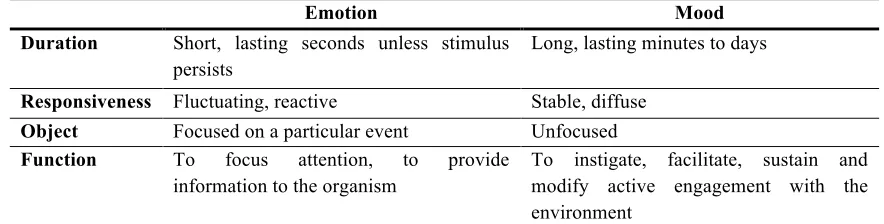
It has been hard for researchers to arrive at a consensual definition of emotion. In recent days, emotion was defined as “episodic, relatively short-term, biologically-based patterns of perception, experience, physiology, action, and communication that occur in response to specific physical and social challenges and opportunities” (Keltner & Gross, 1999, p.468), or similarly as “transient, bio-psychosocial reactions designed to aid individuals in adapting to and coping with events that have implications for survival and well-being” (Sander & Scherer, 2009, p.69). These definitions commonly emphasize that emotion is (a) a transitory condition with (b) biological and perceptual reactions (c) in order to manage a given situation. Emotion should not be confused with ‘mood’ or ‘temperament’, as mood or temperament is not a specific response to anything, but rather a long-lasting state. It is normally induced by sustained exposure to affective stimuli and lasts for longer time periods (Bradley & Lang, 2000). Table 1 summarizes the difference between emotion and mood. On the other hand, ‘affect’ is “a general term that has come to mean anything emotional”, in the science of emotion (Barrett & Bliss‐Moreau, 2009).

Table 1 Comparison of ‘emotion’ and ‘mood’

Emotion Mood

Duration Short, lasting seconds unless stimulus

persists

Long, lasting minutes to days

Responsiveness Fluctuating, reactive Stable, diffuse

Object Focused on a particular event Unfocused

Function To focus attention, to provide

information to the organism

To instigate, facilitate, sustain and modify active engagement with the environment

(15)

There have been various emotion theories and concepts that explain the whole range of emotions comprehensively. In a broad sense, two different frameworks for emotion model will be discussed in the following sections: the first is constructionist vs. basic vs. appraisal theory debate on the cognitive system of emotion, and the second is neural model debate between functionalists and constructionists.

2.1.1. Constructionist Theories vs. Basic Emotion Theories vs. Appraisal Theories According to the early constructivist (constructionist) theory by Schachter and Singer (1962), an emotional state is based on two factors: ‘cognition of arousing situation’ and ‘perceived physiological arousal’ produced by stimuli. People evaluate the situational context and infer appropriate emotion to feel based on these arousals (Mandler, 1990). More recent constructivist theory (Barrett, 2006) stated that ‘core affect’ and ‘conceptualization’ shape mental states. A basic rule is that core affect, caused by a large number of different factors, is made meaningful through categorization (conceptualization) and develops into an emotional feeling. In this model, the connection between core affect and conceptualization is based on situational factors and socio-cultural factors stored in memory.

Ekman’s basic emotion model (Ekman & Friesen, 2003; Izard, 1991), on the other hand, argues that emotions categories are separate entities, given by the structure of the neuronal system. According to the model, a certain type of event is automatically appraised via database lookup and one of basic emotions is determined. Thus, it is relatively deterministic in a macro level.

(16)

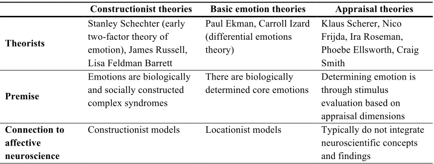
in the process of producing core affect, because the constructionist process includes appraising somatosensory feedbacks as well as situational meaning. However, constructionists do not accept the micro-level deterministic process of the appraisal model. Table 2 compares aforementioned theories.

Table 2 Comparison of emotion theories

Constructionist theories Basic emotion theories Appraisal theories

Theorists

Stanley Schechter (early two-factor theory of emotion), James Russell, Lisa Feldman Barrett

Paul Ekman, Carroll Izard (differential emotions theory)

Klaus Scherer, Nico Frijda, Ira Roseman, Phoebe Ellsworth, Craig Smith

Premise

Emotions are biologically and socially constructed complex syndromes

There are biologically determined core emotions

Determining emotion is through stimulus evaluation based on appraisal dimensions

Connection to affective neuroscience

Constructionist models Locationist models Typically do not integrate neuroscientific concepts and findings

2.1.2. Locationist Models vs. Constructionist Models

(17)

There are roughly two different views on this matter. It was suggested that emotions are processed by either specialized and separate centers or motor and sensory centers that are already assigned to specific functions. The former shape the locationist account and the latter forms constructionist account. Many of the recent emotion research made locationist assumptions and tried to distinguish different cortical and subcortical activity signature for each emotion (Lindquist et al., 2012). The hypothesis is that people have internal mechanisms for discrete emotion entities, and there is individual neural structure (e.g., Baumann & Mattingley, 2012; Calder, Keane, Manes, Antoun, & Young, 2000; Pessoa & Adolphs, 2010) or neural networks specialized for each emotion (e.g., Panksepp, 2011; Pessoa, 2012; Phillips et al., 1997) like Ekman’s basic emotion model. However, a great deal of studies failed to find consistence evidence for distinct anatomical patterns that distinguishes emotional categories (Lindquist et al., 2012; e.g., Mauss & Robinson, 2009; Vytal & Hamann, 2010).

(18)

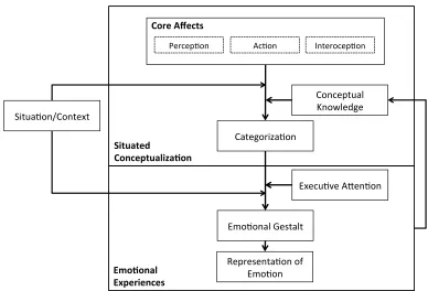
The constructionist model is connected to the constructionist theory mentioned in the previous section. According to the model, emotional experiences occur when person conceptualizes an instance of affective feeling, based on their conceptual knowledge (Barrett, 2006). The process can be decomposed into small brain networks that generate and represent core affect, categorize based on situation and experience, and support executive attention to retrieve concepts (Kober et al., 2008; Lindquist et al., 2012; Oosterwijk et al., 2012; Wilson-Mendenhall, Barrett, & Barsalou, 2013). Activation of these networks changes in real time as individual’s body feelings or situation changes.

Core affect is a basic unit of emotion (Barrett & Bliss‐Moreau, 2009; Russell & Barrett, 1999; Russell, 2003). Sensory inputs, such as raw somatic, visceral, vascular, and motor cues arousal interact together and the brain makes and initial top-down prediction about the meaning of the inputs (Bar, 2003). To produce a unified concept, errors between bottom-up information from core affect and top-down prediction is minimized (Friston, 2010). It is done by modifying prediction to fit to the situation or behavioral plan (Barrett, 2006) and to the stored representations of prior experiences, such as memories or language (Wilson-Mendenhall et al., 2013). Words take part in conceptualization when perceivers make meaning out of core affects, as language plays an important role in integrating different states into one category (Gentner & Goldin-Meadow, 2003).

(19)

Figure 1 A simplified diagram of constructionist model

2.1.3. Implications for the Present Study

Emotion studies have explicitly or implicitly supported one of these affective processing models. Studies about facial expressions commonly added evidence to the basic, appraisal, and locationist models (e.g., Izard, Huebner, Risser, & Dougherty, 1980; Tracy & Robins, 2004; Young et al., 1997). On the contrary, many literatures observed that there is no distinct neural signature for discrete emotions. Emotional process might not be a separate function for emotion, but a part of general mental process. This study favors the latter constructionist view that admits innate variability of emotion as a general mental process and emotions’ potential connection with other brain functions. By doing this, we will be able to see if human emotions are directly connected to human performance in neural level.

Categoriza*on, Situa*on/Context,

Emo*onal,Gestalt,

Conceptual, Knowledge,

Situated(

Conceptualiza0on(

Representa*on,of, Emo*on, Emo0onal((

Experiences(

Execu*ve,A?en*on, Core(Aﬀects(

(20)

2.2. Emotion Categories

2.2.1. Classification of Emotions

Basic emotions proposed by Ekman include anger, disgust, fear, enjoyment, sadness and surprise (Ekman & Friesen, 2003). However, because it is difficult to encompass all other possible types of affective phenomena, such as joy, pride, amazement, tenderness, frustration, anguish, despair, shame, or panic, researchers have used various criteria to classify emotions in previous studies. Circumplex models place discrete emotions on the circle, based on their similarity or relatedness. The two perpendicular dimensions in a circle varied by model: Russell (1980) used arousal-valence dimension, Watson & Tellegen (1985) used engage-valence dimension, and Thayer (1989) used tension-energy dimension. Shaver et al. (1987), on the other hand, classified emotional words using a hierarchical cluster analysis. There also have been many trials to assign discrete emotion in a certain dimensional space such as SAM (Self-Assessment Manikin), PAD (Pleasure-Arousal-Dominance by Mehrabian, 1996), and PANAS-X (Positive Affect Negative Affect Scale by Watson & Clark, 1999). These are not mutually exclusive, but developed based on each other.

2.2.2. Stimulus for Experiments

Stimuli for the experiments had been mostly visual or auditory. It was known that detecting and interpreting of affect in the human voices is a complex issue (Banse & Scherer, 1996; Zinken, Knoll, & Panksepp, 2008) and affective information is communicated via nonlinguistic parts (Scherer & Wallbott, 1994), most studies have used emotionally affective images. Short presentation of picture stimulus could produce emotion, with non-affective components (noise) minimized.

(21)

Behavioral Activation System (BAS) and Behavioral Inhibition System (BIS) scales (Beck, Smits, Claes, Vandereycken, & Bijttebier, 2009; Bijttebier, Beck, Claes, & Vandereycken, 2009) classify emotions into two motive systems: aversive that result in withdrawal behaviors, and appetitive that lead to approach behaviors. It is similar to the preservative vs. protective system (Konorski, 1967) or attractive vs. aversive system (Dickinson & Dearing, 1979). For example, fear and sadness were differed from anger (same valence, but anger expresses approach motivation) in terms of brain responses (Hoekert, Bais, Kahn, & Aleman, 2008; Van Rijn et al., 2005). This indicates that underlying activation of neural circuits could show different patterns, even though two emotions are similar in arousal and valence dimensions.

Standardized stimulus set allows standardized emotion testing. It can help identifying the effect of different tasks, personality, environment, and so forth. However, there is a lack of such database for discrete emotions. Mikels’ norm (2005) is the one that identifies IAPS images that elicit one discrete emotion more than others. Discrete emotional terms used in this database were: amusement, awe, contentment, excitement, anger, disgust, fear, and sadness. Some were undifferentiated, and some image evoked emotion that overlapped between more than two emotions. The present study focused on such discrete emotions to reveal variances in emotional processes of between emotions, as they can possibly affect a certain type of human performance differently, such as risk-related behaviors (Cavicchio & Poesio, 2012), or coping with workload, stress, and exhaustion (Lee & Lee, 2001). It can also guide the discrete affective design of various interfaces. The use of discrete emotion database will help studying such effects.

2.3. Individual Differences in Affective Processing

2.3.1. Determinants of Affective Processing

(22)

age, genetic factors, or hormonal influences are the main sources (see Toga & Thompson, 2003), and personality traits such as neuroticism, extraversion-introversion, or mood state are other sources (Gale, Edwards, Morris, Moore, & Forrester, 2001; Lim, Woo, Bahn, & Nam, 2012). Table 3 shows how these factors influence brain activity. A limitation of these personalities, however, is that they cannot directly influence emotional process. For example, sad mood disturb emotional processing by impeding global information processing (Schmid, Schmid Mast, Bombari, Mast, & Lobmaier, 2011).

Table 3 Determinants of affective processing

Factors Effect

Handedness Right-handed individuals show more left hemisphere activation in speech and language

comprehension (Toga & Thompson, 2003)

Gender Females show more rapid reaction to emotional stimuli. Valence effect is greater in

female, and arousal effect is greater in male (Lang, Greenwald, Bradley, & Hamm, 1993)

Age Adults show more regulation on negative emotions, compared to younger individuals (Wood & Kisley, 2006)

Genetic Factor Heredity plays an important role in structuring the cortex (Thompson et al., 2001)

Personality More neurotic individuals showed more hemispheric asymmetry, and extravert

individuals showed less activation of cortex (Gale et al., 2001)

Mood State Highly disturbed mood affected enhanced lateralization (Lim et al., 2012)

2.3.2. Emotional Granularity

(23)

trait-level individual difference in cognition: people with high granularity may apply more complex conceptual knowledge to conceptualize their internal state, while people with low emotional granularity may experience emotion only as positivity-negativity. High granular people access and use their conceptual knowledge more efficiently to conceptualize affective state using greater working memory capacity (Barrett et al., 2004). Deterioration of negative feeling was faster in highly granular individuals (Sevdalis, Petrides, & Harvey, 2007). On the other hand, extremely low granularity, or failure of situational conceptualization may result in alexithymia (an inability to identify and name emotional states, Taylor & Bagby, 2000).

(24)

2.4. Event-Related Potential (ERP)

There exist numerous feature extraction and translation techniques. Introduced here is ERP, which shows the intensity change of electrical activity on scalp. As the fluctuation of electrical power is represented on time domain, it benefits from high temporal resolution of EEG method.

(25)

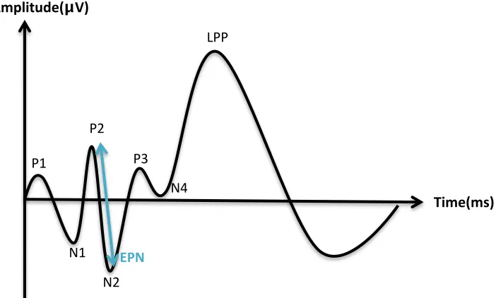
Figure 2 Typical ERP waveform and components in response to affective visual stimuli

In general, the effect of affective stimuli started early and generated early ERPs (around 170ms), primarily reflecting uncontrolled spontaneous perceptual processing. It is a common view that affective contents are processed after at least 100ms, although some researchers observed additional earlier ERP components (before 100ms) that are discriminable between emotions (e.g., Pourtois, Grandjean, Sander, & Vuilleumier, 2004; Rigoulot et al., 2008). The amplitude grows stronger around 300ms through 700ms range, and remains consistent until around 850ms. These late ERPs are thought to reflect increased cognitive resource allocation facilitated by motivational relevance of cues (Codispoti, Ferrari, & Bradley, 2007). In terms of topography, frontal areas were involved in more complex cognitive processes such as evaluation of emotional valence (e.g., Davidson & Tomarken, 1989; Davidson & Irwin, 1999), and parietal areas were involved in analyzing emotional arousal (Heilman, Lane, & Nadel, 2000; Heller, 1993; LaBar & Cabeza, 2006). Olofsson, Nordin, Sequeira, & Polich (2008) is good for comprehensive ERP review.

N4# P3#

LPP#

N2# P2#

N1# P1# Amplitude(μ

V)-

(26)

EPN-2.4.1. Short Latency

Early components (N1 or P1 in 100-200ms range) are sensitive to perceptual factors of a stimulus. It indicates sensory processing within the visual cortex, such as the mapping of the distinctive object features (Balconi & Pozzoli, 2003). Thus, early components index structural elaboration of stimuli or selective attention (e.g., Batty & Taylor, 2003; Bradley, 2009; Junghöfer, Bradley, Elbert, & Lang, 2001; Schupp, Stockburger, Codispoti et al., 2007). This is not inconsistent with the results of some studies that found that emotional stimuli elicited larger positive amplitudes as opposed to neutral stimuli, in frontal area (e.g., Eimer, Holmes, & McGlone, 2003).

Threatening features, in specific, captured more attention (Codispoti, Ferrari, Junghöfer, & Schupp, 2006; Schupp et al., 2004). Fearful stimulus sometimes exhibited faster reaction than other emotional stimuli (Eimer et al., 2003). Threating stimulus was processed even when one was instructed to ignore the meaning of words (Thomas et al., 2007). Thus, it has been assumed that the greater potential of risk in negative affect (Baumeister, Bratslavsky, Finkenauer, & Vohs, 2001) engaged more attentional processing and had favored access to processing resources (Dolcos & Cabeza, 2002). The early ERP components were also sensitive to erotic images (De Cesarei & Codispoti, 2006; Flaisch, Junghöfer, Bradley, Schupp, & Lang, 2008; Schupp, Junghöfer, Weike, & Hamm, 2003). However, there exists controversy in whether the early components’ different reaction to negative and positive is due to stimulus’ emotional contents or due to visual features. Also, the studies failed to show distinctive neural patterns for other discrete emotions in early stage.

(27)

Dolan, 2003). Sabatinelli, Lang, Bradley, Costa & Keil (2009) suggested that amygdala and inferior temporal cortex differentiate emotional from non-emotional scenes. Overall, affective content are analyzed causing the reorientation of attention and direct the later process (Delplanque, Silvert, Hot, Rigoulot, & Sequeira, 2006).

2.4.2. Middle Latency

Middle ERP components (N2 or P2 between 200-300ms) represent selection processes. Especially, the P2 is one of the visually evoked response patterns associated with the analysis of higher-level visual features guided by attention (Luck & Hillyard, 1994). Selective attention to task related features or biologically relevant properties lead to the process of arousal and hedonic value of emotional stimuli (Balconi & Pozzoli, 2003). Due to the P2 component’s reaction to salient stimulus, or strongly affective stimulus, previous research has indicated that this component may originate in the anterior cortices (Potts & Tucker, 2001).

The negative peak around 300 ms (N2) also has been proposed as a good candidate of discovering emotional effects (Carretié, Iglesias, Garcia, & Ballesteros, 1997). Enhanced negativity appeared significantly at lateral temporal and occipital electrodes. For example, fearful images showed enhanced negativity in lateral posterior area (Eimer et al., 2003). This increased early posterior negativity (EPN) was mainly elicited by highly arousing stimuli (Schupp et al., 2004; Schupp, Flaisch, Stockburger, & Junghöfer, 2006a; Schupp, Junghofer, Weike, & Hamm, 2003) and was correlated modestly with signal modulations in the amygdala and anterior cingulate cortex (ACC) (Sabatinelli, Keil, Frank, & Lang, 2013). Asymmetry was not yet apparent in these early stages, although reported inconclusively (De Cesarei & Codispoti, 2006; Keil et al., 2001).

2.4.3. Long Latency

2.4.3.1. P300

(28)

peak happens over parietal area, associated with target processing (Sabatinelli, Lang, Keil, & Bradley, 2007). It has been suggested to be the result of various cognitive functions such as: short-term memory storage (Palomba et al., 1997; Polich, 2007), contents evaluation (Knight, 1997; Soltani & Knight, 2000), and decision-making processes (Nieuwenhuis, Aston-Jones, & Cohen, 2005). In previous emotion studies, higher amplitude of P3 was obtained from highly emotional and arousing stimuli (e.g., Conroy & Polich, 2007). Highly arousing pictures were perceived to be more interesting, and been remembered better (Cuthbert, Schupp, Bradley, Birbaumer, & Lang, 2000), as they potentiated attention (Schupp et al., 2007). Although it was observed that the negative and positive stimuli shared some cognitive resources, negative emotions obtained a higher processing priority and take up processing capacity (Meinhardt & Pekrun, 2003). Other than emotional factors, intentional attention or perceived importance of stimulus further intensified the amplitude of P3, while non-evaluative categorization task decreased the amplitude of P3 (Kok, Ridderinkhof, & Ullsperger, 2006; Ridderinkhof, van der Molen, Maurits W, Band, & Bashore, 1997). Prior experiences were reflected in the P3-related physiologic activity. For example, maltreated children showed larger P3 amplitude when they attended to angry face, opposed to happy targets (Pollak, Cicchetti, Klorman, & Brumaghim, 1997). It indicated that P3 is more controlled stages of processing (Thomas et al., 2007). Thus, suggested was that P3 is related to more cognitive implications than to affective processes in some studies (Carretié, Iglesias, Garcia, & Ballesteros, 1997).

2.4.3.2. N400

(29)

previous semantic memory (Laszlo & Federmeier, 2011). Emotional valence also contributed to this semantic process (Schirmer & Kotz, 2003).

2.4.3.3. Late Positive Potential

A component that appears later and lasts long with widely distributed positive peak amplitude is commonly found and called the late positive potential (LPP) (Schupp et al., 2000). The amplitude of LPP was related to memory performance and other top-down processing in many studies (e.g., Azizian & Polich, 2007). In emotion studies, emotionally arousing pictures elicited larger LPPs (Codispoti, Mazzetti, & Bradley, 2009; Cuthbert et al., 2000; Schupp, Flaisch, Stockburger, & Junghöfer, 2006), particularly greater amplitude in left centro-parietal area to negative words (Inaba, Nomura, & Ohira, 2005). Some kind of emotional regulation (lower LPP) was also observed in older adults group (Wood & Kisley, 2006), suggesting controlled top-down process in this time frame. On the other hand, Carretie et al. (1997) found that increased ERP amplitude evoked motor effects as well as perceptual processes. A recent EEG and fMRI study revealed that LPPs represent the collective activity of visual cortex (Sabatinelli et al., 2013) and are supported by the iterative feedback from subcortical to cortical sites, resulting in a series of attention orienting, metabolic mobilization, and action preparation (Lang & Bradley, 2010; Pessoa & Adolphs, 2010; Vuilleumier, 2005), with combined activity of striate cortex, inferior temporal cortex, and medial parietal cortex (Sabatinelli et al., 2007).

ERP components show the people’s behavior in the neural level. We could directly notice how individuals actually perceived the stimulus, how fast they reacted, and to what extent the stimulus impacted the person.

(30)

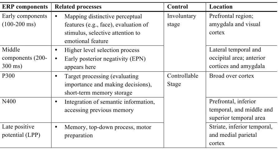
2003 (oddball task)), and analysis methods (peak amplitude, average amplitude around peak, etc.), they showed variable ERP outcomes. Nonetheless, each components and associated functions have been illustrated through a large number of experiments. Table 4 summarizes common conclusion of previous studies, and more ERP experiments are listed in Appendix H.

Table 4 ERP components and related cognitive processes

ERP components Related processes Control Location

Early components (100-200 ms)

• Mapping distinctive perceptual features (e.g., face), evaluation of stimulus, selective attention to emotional feature

Involuntary stage

Prefrontal region; amygdala and visual cortex

Middle

components (200-300 ms)

• Higher level selection process • Early posterior negativity (EPN)

appears here

Lateral temporal and occipital area; anterior cortices and amygdala P300 _• Target processing (evaluating

importance and making decisions), short-term memory storage

Controllable Stage

Broad over cortex

N400 _• Integration of semantic information, accessing previous memory

Prefrontal, inferior temporal, and middle and superior temporal area Late positive

potential (LPP)

• Memory, top-down process, motor preparation

Striate, inferior temporal, and medial parietal cortex

(31)

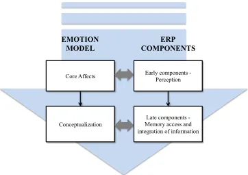
Figure 3 Constructionist emotion model and corresponding ERP components

2.5. Coherence

EEG activity shows difference oscillation in at various frequency bands, and each frequency band react differently to emotional stimuli. Coherence is the measure that shows the strength of synaptic connections between two distant brain regions within certain frequency bands. This long-range dynamic synchrony between groups of neuronal assemblies is thought to be an important central mechanism of information processing between multiple brain areas that help spontaneous functioning of brain (Bhattacharya, Petsche, Feldmann, & Rescher, 2001). High coherence is often interpreted as dependency, correlate of cognitive processing (Thatcher, Krause, & Hrybyk, 1986), anatomical connections (Fein, Raz, Brown, & Merrin, 1988), temporal correlation (Singer & Gray, 1995), mutual information exchange (Petsche & Rappelsberger, 1992), and functional cortical integration (Maurits, Scheeringa, van der Hoeven, & de Jong, 2006), whereas low

Core Affects

Conceptualization

Early components - Perception

Late components - Memory access and integration of information

EMOTION MODEL

(32)

2.5.1. Theta Band (4-8 Hz)

Coherence measurement is specific to frequency bands. In general, low frequency bands reflect attention and working memory processes in frontal and parietal areas (Jensen & Tesche, 2002; Klimesch, 1999). Theta rhythm is thought to be responsible for the encoding of new information (Klimesch, Doppelmayr, Russegger, & Pachinger, 1996) and emotional process, especially fear conditioning (Knyazev, 2007; Putman, van Peer, Maimari, & van der Werff, 2010). Some studies reported early synchronization of theta wave when participants are viewing emotional images (Aftanas & Golocheikine, 2001; Balconi & Pozzoli, 2009; Balconi, Brambilla, & Falbo, 2009; Knyazev, Levin, & Savostyanov, 2008), listening to music (Sammler, Grigutsch, Fritz, & Koelsch, 2007), and watching films with emotional content (Jausovec, Jausovec, & Gerlic, 2001).

2.5.2. Alpha Band (8-13 Hz)

In the early stage of EEG study, Ray and Cole reported that alpha power (or mu) is related to attentional demand (Ray & Cole, 1985). Alpha power mostly decreases when cortical excitability and engagement in stimulus processing increases (e.g., Andrew & Pfurtscheller, 1996; Cooper, Croft, Dominey, Burgess, & Gruzelier, 2003; Klimesch, Sauseng, & Hanslmayr, 2007; Sauseng & Klimesch, 2008). Therefore, as task gets complex and requires more attention, the magnitude of alpha suppression increases. Recently proposed theory suggests that alpha band is related to the disengagement of task-irrelevant brain areas (Palva & Palva, 2007). In emotion research, high coherence of theta and alpha band in fronto-parietal area reflected central executive function of working memory (Sauseng, Klimesch, Schabus, & Doppelmayr, 2005).

2.5.3. Beta Band (13-30 Hz)

(33)

recent studies associated beta rhythm with attentional top-down processing that predominate the effect of novel external events (von Stein, Chiang, & Konig, 2000). It is capable of long-distance coupling (Schnitzler & Gross, 2005). Based on these characteristics, Engel and Fries (2010) suggested that beta rhythm is related to the maintenance of status quo, the current cognitive or sensorimotor state.

2.5.4. Gamma Band (30-50 Hz)

Recently gamma wave (30 Hz and higher) has captured most attention. It was observed that gamma oscillations are related to a broad range of processes such as feature integration, attention, stimulus selection, integration sensory inputs and sensorimotor activities, movement preparation, and memory formation (Engel, Fries, & Singer, 2001; Jensen, Kaiser, & Lachaux, 2007; Knyazev, 2007; Senkowski, Schneider, Tandler, & Engel, 2009) were affected by gamma rhythm. It also showed increased power in visual stimulation task or movement tasks (Murthy & Fetz, 1992; Pfurtscheller, Graimann, Huggins, Levine, & Schuh, 2003). These faster oscillations might serve active information processing by actively coupling cell assemblies over spatially separated regions and binding attributes and object representations (Tallon-Baudry & Bertrand, 1999; Varela, Lachaux, Rodriguez, & Martinerie, 2001). In emotion study, the 30-50 Hz band showed more power over left hemisphere for negative valence and more power of right hemisphere for positive valence. In particular, right frontal electrodes showed enhanced gamma power for emotional pictures (Keil, Muller, Ray, Gruber, & Elbert, 1999). Li and Lu (2009) successfully classified people watching happy and sad facial expressions with 93% accuracy using gamma band power.

(34)

can be modulated by individual traits such as gender, personality, and implicit/passive condition of tasks. In addition, it is very difficult to directly associate oscillatory activity to a unique cognitive function. Still, studying coherence will help us picture the coherent activity of different brain regions and corresponding functions. Table 5 is a brief summary of functions of each frequency band.

Table 5 Frequency bands and related cognitive functions

Frequency Band Functions

Theta (4-7 Hz) Encoding of new information, fear conditioning

Alpha (8-12 Hz) Attention, working memory, disengagement of task-irrelevant brain areas Beta (13-30 Hz) Sensorimotor and motor functions, maintaining status quo

Gamma (30-50 Hz) Integration of information

2.6. Research Questions and Hypotheses

Research question 1 and 2 are related to the model of emotion. The present study tried to find evidence of constructionist emotion model, by using discrete emotional category for emotional evocation. Research question 3 and 4 are about how individual difference in emotional granularity influences emotional process.

• Research Question 1: Do different emotional contents undergo different neural

process? Which emotion model better explains the neural process of emotion?

o Hypothesis 1: In order to support the constructionist model and reject locationist model, the activation of specific brain region will not be dependent on discrete emotions. In other words, there will be no interaction effect between discrete emotion and brain locations.

o Hypothesis 2: The ERP components will show difference between emotions, reflecting discrete emotional processing.

• Research Question 2: How does the emotional granularity influence the emotional

processes?

(35)

o Hypothesis 3B: The late ERP components will show granularity effect because granularity requires higher-level cognitive process of labeling affective states. More granular individuals will demonstrate greater reaction to each ERP component.

o Hypothesis 4: Granularity will have effect on coherence distribution, especially those associated with emotional regulation. Highly granular person will show greater change of coherence between two brain areas, through where affective experience is controlled.

2.7. Summary

(36)

3. METHODOLOGY

3.1. Participants

The total of 28 participants from a local university participated in the EEG experiment. The population was restricted to male to avoid sex difference confounds (e.g., Kring & Gordon, 1998). All participants were asked to finish online survey on the day before the EEG recording, and also finish a stimulus rating survey after the EEG recording. They were compensated with class credit, and all subjects signed an informed consent form prior to the beginning of the EEG recording. The Institutional Review Board at NCSU approved the human study protocol. See appendix C for the approved IRB approved consent form.

Out of 28 male participants, 8 were excluded from the data analysis, in order to avoid unexpected distortion of data. Three participants were excluded from analysis based on the online survey results: one left-handed or ambidextrous participant and two anxious / depressed participants (were moderately anxious or had potential of concern or more than mildly depressed). These participants were screened because handedness influences the lateralization of brain (Toga & Thompson, 2003), and high anxiety and depression exhibit greater reaction to negative images than those who are not (Oathes et al., 2008; Lang, Bradley, & Cuthbert, 1998). One participant stated attention deficit hyperactivity disorder (ADHD) and his data was also removed. There were four participants removed due to data recording errors. As a result, brain signals from 20 right-handed male participants without severe anxiety or depression were analyzed. The average age of 20 participants was 21.05 years and standard deviation was 1.19 years.

3.2. Apparatus

3.2.1. Online Survey

(37)

they want, and could come back later to the same page as long as they use the same computer and browser. Data from all participants were saved in one file and analyzed with R, a language and environment for statistical computing and graphics from GNU Project. Table 6 shows which survey collected which information. See Appendix D for the survey details and section 3.3.1 for calculating granularity from DRM survey. The survey was anticipated to take approximately 45 minutes to complete.

Table 6 Online surveys

Information collected Surveys

Gender and age Demographic survey

Handedness Edinburgh Handedness Inventory

(EHI, Oldfield, 1971)

Anxiety level Beck Anxiety Inventory

(BAI, Beck & Steer, 1991)

Depression level Beck Depression Inventory

(BDI, Beck, Steer, & Carbin, 1988)

Emotional Granularity

Day Reconstruction Method

(DRM, Kahneman, Krueger, Schkade, Schwarz, & Stone, 2004)

3.2.2. Experimental Stimuli

3.2.2.1. IAPS and Mikels’ Norm

(38)

Awe (#5300) Excite (#8220) Fear (#1931) Disgust (#9290) Neutral (#7041)

Figure 4 Examples of IAPS images for each discrete emotion

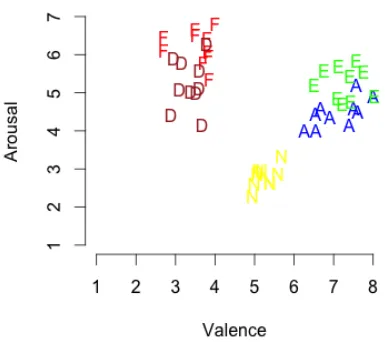
Valence and arousal of each image is plotted in the Figure 5. Negative images had low valence and high arousal. Positive images had high valence and high arousal. Awe and Excite images were not differ in valence (t(9)=-0.8025, p=0.4429) but differ in arousal (t(9)=-3.6058, p=0.0056).

Figure 5 IAPS images on valence-arousal space (A: Awe, E: Excitement, F: fear, D: disgust, N: neutral)

(39)

(a) (b)

Figure 6 Discrete emotion scores from Mikels’ norm (2005): (a) awe and excite, and (b) fear and disgust

3.2.2.2. Validation of Stimuli

We needed to validate the use of stimuli. First, in order to see if emotional stimuli chosen from IAPS and discrete emotion assigned to each image based on Mikels’ norm successfully evoked intended emotion to participants, a survey was done after the EEG data collection. The participants completed a survey that asked what emotion they felt while they were watching each image on the TV screen. They chose one emotional word from neutral, awe, excite, fear, and disgust, and specified the strength of selected emotion (on a 0 to 6 scale). If they could not find an emotional word that fits their experience, they were allowed to leave it blank or write down an alternative emotion. If they did not to answer, chose more than two words, or indicated other emotion, the response was discarded. If a participant rated the image as intended, it was considered successful elicitation of the emotion. The proportion of successful elicitation was calculated over participants to validate the emotion that each picture induces. Table 7 shows what percentages of images were successful in producing the emotion from Mikels’ norm (2005). Not all images could evoke intended emotion to all participants. However, the majority of images elicited intended emotion to most of the

0" 2" 4" 6"

Aw

e$

Exc(e$

Awe" Excite"

0" 2" 4" 6"

Fe

ar

%

Disgust%

(40)

Table 7 Intended emotions based on Mikels’ norm and the percentage of perceived emotion for each discrete intended emotion

Perceived Emotion

Awe Excite Fear Disgust Neutral

Intended Emotion (Mikels’ norm)

Awe 72.5% 8.5% 0.0% 0.0% 19.0%

Excite 8.0% 65.0% 1.0% 0.0% 26.0%

Fear 22.0% 6.0% 52.5% 1.5% 17.5%

Disgust 9.0% 6.0% 7.0% 63.0% 14.5%

Neutral 13.5% 4.5% 2.0% 0.5% 79.5%

Average level of emotion

(0-6) 2.99 2.80 2.65 3.20 N/A

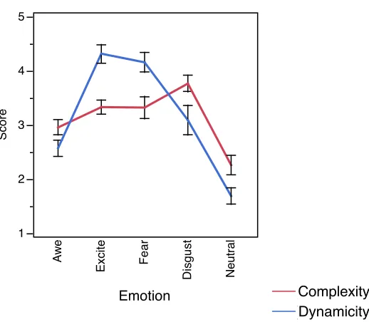
Second, visual feature of chosen image is a potential factor that can affect brain activity. A mini online survey with 25 participants (not overlapping with this experiment) was done with the same online survey platform ‘Qualtrics’, in order to see if images in discrete emotion categories have different visual characteristics. Each participant rated ‘complexity’ and ‘dynamicity’ of all 50 images, because it was reported that figure-ground images and scene affect early ERP components around 150ms (Bradley, Hamby, Low & Lang, 2007), and dynamic actions in pictures enhance movement-related brain areas (Riva & Zani, 2009). The result of this survey was used in section 5.1.1.

In the survey, they were asked, “please rate this picture: this picture is simple/complex”, and asked to chose the level among five numbers, “1: very simple, 5: very complex”. Again it asked, “this picture is static/dynamic”, and asked to rate using five numbers again, “1: very static, 5: very dynamic”.

(41)

category varied in terms of dynamicity (F(4, 45) = 32.67, p < .0001). In short, there were three levels of dynamicity level: fear and excite were most dynamic, disgust and awe were less dynamic, and neutral was the most static. In detail, neutral stimuli were static than excite (p<.0001), fear (p<.0001), disgust (p<.0001), and awe (p=0.0027). Awe was more static than excite (p<.0001) and fear (p<.0001). Excite and fear was more dynamic than disgust (p<.0001). Figure 7 shows the result of the survey. Each error bar is constructed using 1 standard error from the mean.

Figure 7 Averaged complexity and dynamicity score of images in each emotional category: blue line represents dynamicity from 1 (very static) to 5 (very dynamic), red line represents complexity from 1

(very simple) to 5 (very complex).

3.2.3. EEG Measurement System and Analysis

3.2.3.1. EEG Recording

Signal was amplified with a g.USBamp amplifier from g.tec Medical Engineering, band-pass filtered between 0.1 Hz and 60 Hz, notch filtered at 60 Hz, and digitized at a rate

1 2 3 4 5

Score

Awe

Excite Fear

Disgust Neutral

Emotion Mean(Complexity)

(42)

between electrodes and scalp. Figure 8 is a screenshot of LabVIEW program developed for EEG recording. Part A was displayed on a 42” television and showed images on a full-screen. Part B and C were displayed on a researcher side’s full-screen. Part B was used to enter participant’s information and overview the status experiment, and part C displayed amplitude of each electrode.

Figure 8 Front panel of EEG recording program

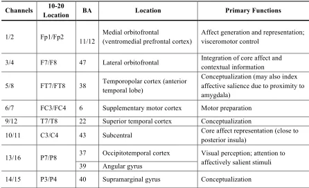
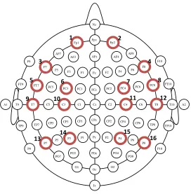
The participants were seated in a comfortable chair in front of the TV, 50” from the TV. Participants wore an EEG cap embedded with 16 electrodes covering Fp1/Fp2, F7/F8, FC3/FC4, T7/T8, P7/P8, FT7/FT8, P3/P4, C3/C4 area, based on the modified 10-20 systems of the International Federation (Jasper, 1958; Niedermeyer & da Silva, 2005). Fpz was used as a ground, and left ear lobe was used as a reference. The areas were chosen based on the Brodmann Area (BA), the list of cerebral cortex areas defined by corresponding functions. Table 8 shows channel numbers, 10-20 locations, corresponding BAs, anatomical locations with functional names, and their functions, derived from meta-analyses of the neuroimaging literature on emotion (e.g., Kober et al., 2008; Lindquist et al., 2012). For montage detail of channels, refer to the Figure 9.

(43)

Table 8 Channels and their functional locations

Channels 10-20

Location BA Location Primary Functions

1/2 Fp1/Fp2

11/12

Medial orbitofrontal

(ventromedial prefrontal cortex)

Affect generation and representation; visceromotor control

3/4 F7/F8 47 Lateral orbitofrontal Integration of core affect and contextual information

5/8 FT7/FT8 38 Temporopolar cortex (anterior temporal lobe)

Conceptualization (may also index affective salience due to proximity to amygdala)

6/7 FC3/FC4 6 Supplementary motor cortex Motor preparation 9/12 T7/T8 22 Superior temporal cortex Conceptualization

10/11 C3/C4 43 Subcentral Core affect representation (close to posterior insula)

13/16 P7/P8 37 Occipitotemporal cortex Visual perception; attention to affectively salient stimuli 39 Angular gyrus

(44)

Figure 9 Montage

Each of 50 images was presented for 3 seconds, after 2 second of cross fixation. After the presentation period, a participant took rest for 10 seconds. If the participant’s brain activity calmed down (more than 95% were within the threshold calculated by brain activity during the rest state), next image showed up after another cross fixation. If more than 5% of signals are outside the threshold, the participant was given maximum 20 seconds of additional rest period. After one session is finished, the participant took 3 minutes rest, and the identical second session started. The image presentation order was awe, excitement, fear, disgust, and neutral.

3.2.3.2. EEG noise filtering

Amplified EEG data collected from scalp electrodes have some signal distortions. These artifacts show different shape and higher amplitudes when compared to

Nz CPz Fpz AFz Fz FCz Cz Pz POz Oz Iz Fp1 Fp2 AF3 AF4 AF7 AF8 F7 F5 _F3

F1 F2 F4 F6

F8 F9

FT9 FT7 _FC5

FC3 FC1 FC2 FC4 FC6 FC8

F10

FT10

A1 T9 T7 C5 C3 C1 C2 C4 C6 T8 T10 A2

TP10 P10 TP8 P8 PO8 O2 PO4

P2 P4 _P6

CP2 CP4 _CP6

TP9 TP7 CP5

CP3 CP1 P9 P7 P5 P3 P1 PO7 PO3 O1

Creative Commons: http://creativecommons.org/licenses/by-sa/3.0/nl/deed.en_GB Author: Marius 't Hart - http://www.beteredingen.nl

1" 2"

3" 4"

5" _6" _7" 8"

9" 10" 11" 12"

(45)

uncontaminated signals. It can be patient-related (e.g., minor body movements, pulse, eye movements, sweating, etc.) or technical (AC power line noise at 50/60 Hz, impedance fluctuation, too much gel or dried electrodes, etc.) (Teplan, 2002). In this experiment, trials with amplitude exceeding ±35 µV measured after stimulus onset were excluded from analysis. The threshold 35 µV is an average of 99.7% confident intervals of all participants. Each confidence interval was calculated by sampling all data points collected during -200 ms ~ 1000 ms epoch and estimating µ±3σ. This value was enough to remove the effect of eye blinks that causes voltage over 60 µV.

Collected EEG data underwent Common Average Reference (CAR) calculation, where average amplitude of signals from every electrode site was used as a reference. This was to detect artifacts caused by electromyography (EMG) or electrocardiography (ECG), as earlobe reference is less likely to sense these noises. An isolated single unit activity does not appear on the CAR, except when the signal is so large and dominates the average (see Ludwig et al., 2009 for a good review). New amplitude was computed using the CAR formula below. !_! represented the amplitude between the ith_{electrode and the earlobe} reference.

!_!!"# ₌_!

! −

1

! !!

!

For zero-adjustment, average amplitudes during the 60 seconds of ‘baseline’ window (!_!) was subtracted from corresponding electrodes.

!_!!"#$ ₌_!

! −!!

(46)

3.2.3.3. Event Related Potential (ERP) Components

As ten images from each of five emotional categories were repeated twice, there were 100 epochs for each participant in total and 20 epochs for each discrete emotion. One epoch started 200 ms before the stimulus onset (0 ms) and lasted until 1000 ms after the stimulus onset. Noises were assumed to have an average of zero. Thus an average of twenty epochs in one emotion category became the representative ERP for the emotion. ERP features (amplitudes and latencies of N1, P2, N2, P3, N4, LPP) were than extracted. The letter P or N indicates polarity, and the number indicates the latency in hundred milliseconds. The components in this experiment were determined after data collection. See section 4.1.

3.2.3.4. Coherence

The objective of coherence analysis is to find correlated cortex areas while the participant is watching an emotional image stimulus. The EEG signal was band-pass filtered to get following four frequency bands: theta (4-7 Hz), alpha (8-12 Hz), beta (13-30 Hz), and gamma (30-50 Hz). Once filtered, epochs staring from -1000ms to 1000ms were obtained from all trials. This epoch was again divided into two: 1000ms before the stimulus onset and 1000ms after the stimulus onset. The epoch was determined to focus on the short effect of emotion within 1000ms, just like ERP. The total of 120 ( !"_! = 120) pairwise comparisons of two channels, X and Y, were be done by Welch method using the following equation.

!_!!(!) and !_!!(!) are the power spectrums of x and y, and !_!"(!) is the cross power spectrum of x and y. The formula returned coherence value over frequency.

!_!" ! = !!"(!)

!

!_!! ! ∗!!_!!(!)

(47)

In specific, beta band coherence of prefrontal and parietal were analyzed. Dorsolateral prefrontal cortex (DLPFC) in Fp1 and Fp2 region plays a role in emotion regulation by modulating posterior perceptual area and sending information to the amygdala (Eippert et al., 2007). The frequency band of interest was beta band (13-30Hz), since beta band oscillation mediates long distance coupling (Schnitzler & Gross, 2005) and attentional top-down processing (von Stein et al., 2000). The calculation was done separately in order to show lateralized effects proposed in previous research (Miskovic & Schmidt, 2010; Reiser et al., 2012). Coherence changes of Fp1 and electrodes on left hemisphere (T7, C3, P3, P7) were averaged to summarize interaction within the left hemisphere. Likewise, coherence changes of Fp2 and electrodes on right hemisphere (T8, C4, P4, P8) were averaged to find connectivity changes within the right hemisphere.

3.3. Experiment Design

3.3.1. Independent Variables

The effect of (a) discrete emotions, (b) brain regions, and (c) emotional granularity were studied throughout the study. Discrete emotions (a) and the results of validation are explained in section 3.2.2. For brain regions (b), refer to the Figure 9.

The (c) emotional granularity was measured based on the results of modified day reconstruction method (Kahneman et al, 2004 modified by Rice & Lindquist, unpublished). The participants were asked to recall up to five episodes from morning, five episodes from afternoon, and five episodes from evening of the day before the survey. For each episode, they were asked: what they were doing, where they were, and whom they were interacting with. Finally, they indicated to what level (from 0 to 6) they experienced each of twenty emotions while they were experiencing the episode. Table 9 shows the emotional words used in this survey. As a result, they rated 20 emotions during up to 15 episodes. See appendix D for more details .

(48)

calculated for each participant. Low ICC value indicates that the participant can differentiate discrete emotional categories and express their emotional experiences with different emotion terms. On the other hand, high ICC value means that the participant use terms interchangeably to communication their emotional state. Thus, the ICCs were subtracted from 1 for ease of interpretation to make higher values correspond to more differentiation, or granularity. Positive granularity and negative granularity was then averaged to make a single granularity value.

Table 9 Emotion words used to measure emotional granularity

Positive Negative

Amusement, awe, contentment, excitement, gratitude, happiness, love, pleased, pride, serenity

Anger, boredom, disgust, dissatisfied, downhearted, embarrassment, fear, gratitude, sadness, tired

The participants’ average positive granularity was 0.81 (SD = 0.13) and the average negative granularity was 0.81 (SD = 0.14). Table 10 shows each individual’s age and granularity score.

Table 10 Participants' information. All participants here are right-handed male without severe anxiety or depression.

Participant # Age Positive

Granularity

Negative Granularity

Average Granularity

1 21 0.98 0.80 0.89

2 21 0.95 0.90 0.92

3 21 0.70 0.79 0.75

4 20 0.72 0.88 0.80

5 23 0.88 0.96 0.92

6 21 0.87 0.72 0.80

7 25 0.89 0.53 0.71

8 21 0.81 0.85 0.83

9 20 0.89 0.73 0.81

10 20 0.74 0.72 0.73

(49)

Table 10 continued

12 21 0.79 0.89 0.84

13 21 0.87 0.96 0.91

14 21 0.62 0.90 0.76

15 20 0.80 0.56 0.68

16 20 0.84 0.94 0.89

17 22 0.85 0.94 0.89

18 20 1.01 0.96 0.98

19 21 0.75 0.67 0.71

20 25 0.61 0.83 0.72

Average 21.05 0.81 0.81 0.81

SD 1.19 0.13 0.14 0.11

3.3.2. Dependent Variables

Dependent variables were EEG response to emotional stimuli: amplitudes and latencies of six ERP components (N1, P2, N2, P3, N4, LPP in this experiment) and coherence of cortex areas (in theta (4-7Hz), alpha (8-12Hz), beta (13-30Hz), and gamma (from 30Hz and up to 50Hz) band). All signals underwent common average referencing for noise filtering and followed the analysis procedure described in section 3.2.3.

3.4. Experiment Procedure

(50)

Figure 10 Experiment procedure

3.5. Statistical Analyses

Following analysis methods were employed to test the hypotheses described in section 2.6:

• Normality test was used to test whether the distribution of ERP amplitude and

latency meet the normality assumption of the analysis of variance (ANOVA). If the data was not normally distributed and not proper for ANOVA, Nonparametric Wilcoxon Test (Mann-Whitney U-statistics) was applied.

• ANOVA was done for Hypothesis 1 and 2 with three parameters: GRAN (granularity; 2 levels; high and low), CHAN (channel; 16 levels; 1 to 16), and EMOT (emotion; 5 levels; awe, excite, fear, disgust, and neutral). Hypothesis 1 paid attention to the interaction effect EMOT*CHAN, and Hypothesis 2 focused on the main effect EMOT.

• Tukey’s HSD test was used for post-hoc analysis, because it has greater power

than the other tests and can maintain the Type I error at the same time (Jaccard, Becker, & Wood, 1984). It found the significant difference between each level of the independent variables.

• Regression was done for Hypothesis 3A, 3B and 4, in order to appreciate the

continuous nature of granularity. In hypothesis 3, changes of ERP components

Dump

1min Session I 3 min Rest Session II

Fix 2s Image Presentation 3s Rest 10s Additional Rest Max 20s

Trial 1 Trial 2 … Trial 50

Ref. 1min

EEG Data Collection Online Surveys

•  Demographic survey •  Handedness test •  Anxiety test •  Depression test •  Granularity test

Rating

(51)