EFFECTS OF STRUCTURAL NONLINEARITY ON PROBABILISTIC
RESPONSE OF A NUCLEAR STRUCTURE
Alidad Hashemi1, Tarek Elkhoraibi2, and Farhang Ostadan3
1 Senior Engineer, Bechtel Corporation, San Francisco, CA ([email protected]) 2 Senior Engineer, Bechtel Corporation, San Francisco, CA
3 Bechtel Fellow, Chief Engineer, Bechtel Corporation, San Francisco, CA
ABSTRACT
This paper examines the effects of structural nonlinearity on the results of probabilistic structural analysis of a typical nuclear structure where structural nonlinearity and soil-structure interaction (SSI) are explicitly included. The evaluation is carried out for a soil and a rock site at 10,000 year, 100,000 year, and 1,000,000 year return periods (1E-4, 1E-5, and 1E-6 hazard levels, respectively). Structural responses including the story drifts and in-structure response spectra (ISRS) are examined. The probabilistic implementation of explicit structural nonlinearity in combination with the SSI effects are demonstrated using nonlinear response history analysis (RHA) of the structure with the foundation motions obtained from elastic SSI analyses, which are applied as input to fixed base inelastic analyses. This approach quantifies the expected structural nonlinearity for the particular structural configuration and provides a robust analytical basis for the estimation of the probabilistic distribution of selected demands parameters both at the design level and beyond design level seismic input.
INTRODUCTION
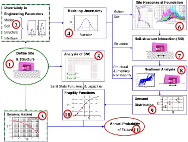
The probabilistic nonlinear analysis described in this paper is part of a comprehensive Integrated Soil-Structure Fragility Analysis (ISSFA) which evaluates the seismic performance of a reinforced concrete shear wall building, typical of nuclear industry structures by quantifying its annual failure probability. The ISSFA methodology is described in Hashemi et al. (2009) and Elkhoraibi et al. (2011). The graphical representation of the ISSFA methodology is presented in Figure 1. This paper discusses boxes 1, 2, 4 through 9 of the depicted methodology.
The subject structure is designed using deterministic analysis to remain elastic at 10,000 year return period seismic hazard level. The uncertainties in the ground motion, site dynamic properties, and linear and nonlinear structural parameters are included in the probabilistic analysis using Latin Hypercube Sampling (LHS) technique with a sample size of 30. For each realization (1 through 30) and each input motion (low frequency (LF) and high frequency (HF) input at each of the 1E-4, 1E-5 and 1E-6 hazard levels), the following 3 stages of analyses are carried out: (1) site response analysis, (2) soil structure interaction analysis, and (3) nonlinear structural analysis. Note that the HF and LF inputs at each hazard level correspond to different seismological events and are analyzed separately. The results from the LF and HF events are combined at the last step of post-processing when component level demands are calculated.
nonlinear models for these walls are calibrated based on available cyclic test data for walls with similar aspect ratios. The development of the nonlinear model and uncertainty considerations in the nonlinear modeling are discussed in Hashemi et al. (2012).
The effects of structural nonlinearity are investigated by considering the structure as a surface-founded structure on two different subsurface conditions corresponding to a deep soil site (VS30 = 1590 fps), and a shallow rock site (VS30=5315 fps). The foundation motion includes the foundation translation along the three orthogonal directions as well as the rigid body foundation rotation about all three directions. Each foundation motion is used as input to a fixed-base nonlinear response history analyses (RHA) of the nonlinear OpenSEES model. Similarly, the foundation motions are also used to perform a set of elastic RHA which provides an elastic control case. The time-history of the base shear, story displacements, element forces, and floor accelerations are obtained from the nonlinear and linear RHA for each realization of LHS at each considered hazard level.
Figure 1. Integrated Soil-Structure Fragility Analysis (ISSFA) Methodology (Hashemi et al., 2009)
STRUCTURAL MODEL
The selected structure, shown in Figure 2(a) is a representative nuclear facilities building with a footprint of about 160 ft by 105 ft on a 6 ft mat foundation at El. 0 ft and supported by reinforced concrete walls ranging in thickness from 2 to 3 ft and the majority of slabs of 2 ft thickness with some exceptions of up to 3 ft slabs. Four major shear walls provide lateral load resistance in the long (East-West (X)) direction of the structure while three shear walls provide resistance in the short (North-South (Y)) direction, as shown in the cross-sectional view in Figure 2(c). The structure consists of 2 main floors extending on the entire footprint at El .33 ft and El. 62 ft, and a third floor occupying the middle 63 ft of the North-South direction and the full width in the other direction at El 80 ft. Steel beams form a platform between El 46 ft and El 62 ft as shown in the middle portion of the structure in Figure 2(b). The roof is at El. 114 ft. The FE model of the structure is developed using shell elements for the mat foundation, walls and slabs. For the purpose of nonlinear analysis, reinforcement ratios are defined for the structure based on the design-basis event demand, calculated using the deterministic SSI approach
1
2
9
8
7
6
5
4
3
10
similar to that described in Hashemi et al. (2011). Story drifts for the structure are calculated in the East-West (X) and North-South (Y) directions along a vertical line at the junction of major shear walls on Col. Line 2 and Col. Line B (node 8188, shown in Figure 2(c)). The ISRS results discussed in this paper are also calculated along the same vertical line. The main structural characteristics for the structure are summarized in Table 1. The fundamental natural frequencies of the structure and their corresponding mass participation factors (MPF) are presented in Table 2.
(a) 3D View (b) First Floor (EL 31.25 ft) (c) Basemat Figure 2. Selected Structure – 3D Views
Table 1. Structure and Model Summary
Footprint 160 ft x 105 ft
Height 114 ft
Embedment Depth 19 ft
Foundation Thickness 6 ft
Slab Thickness 2 to 3 ft
Wall Thickness 2 to 3 ft
Total Weight 76800 kips
Foundation Area 15500 ft2
Average Soil Pressure 4.95 kip/ft2
Concrete Elastic Modulus 3950 ksi
Table 2. Major Fixed Base Modal Frequencies
Direction 1st Mode 2nd Mode 3rd Mode
Frequency MPF Frequency MPF Frequency MPF
East-West (X) 6.0 Hz 32% 8.4 Hz 17% 10.5 Hz 8%
North-South (Y) 5.3 Hz 18% 6.3 Hz 18% 9.5 Hz 26%
The shear walls in the building have height to length ratios of less than 1 (squat shear walls) and are flexurally very stiff about their major axes. Therefore, the lateral dynamic response of the subject structure is governed by the shear deformation of the walls with little contribution from bending. For the purpose of seismic Probabilistic Risk Assessment (PRA), the FE model described above is converted to a more simplified model where all shear walls are represented by vertical elastic beam elements (stick model). The in-plane and out-of plane cross section properties of each stick is calculated for the cross section of their corresponding concrete wall (total of 35 sticks) in the FE model and placed at the center of rigidity of its corresponding concrete wall. Note that the FE representations of the floor concrete slabs in the FE model are not altered in the stick model. The connection between the sticks and floor concrete slab are provided by in-plane rigid beams along the length of each wall at the concrete floor location, therefore, the torsional characteristics of the FE model are maintained in the stick model. The schematic views of the FE model and the stick model of the structure are provided in Figure 3. These figures also show the major structural walls on column lines 2 (X direction) and B (Y direction), respectively.
The adequacy of the stick model is verified by comparing major natural frequencies, mass participation factors, and mode shapes of the stick model with those of the FE model as well as
N N
Node 8188
N Node 8188
comparing the displacement time-history and maximum displacements at different elevations in the structure. These comparisons are documented in Elkhoraibi et al. (2012) and confirm a very good agreement between the global results of the two models with the difference limited to only 12%. Also it was noted that in most cases the stick model is resulting in slightly more conservative displacements.
(a) FE model – Col. line 2 (b) Stick model – Col. line 2
(c) FE model – Col. line B (d) Stick model – Col. line B Figure 3.Comparison of the FE and Stick Model
The lateral load resisting system in the structure consists of shear walls with aspect ratios of less than 1.0 in both X and Y directions. The expected structural nonlinearity in this structure is therefore, entirely due to the nonlinear in-plane shear response of the walls. The flexural response of the walls is confirmed to remain within the elastic range. The median strength of these walls is obtained from the capacity formulation for low-rise concrete shear walls (aspect ratio ) in ASCE 43-05 (2005). Since the intent is to obtain the best estimate capacity of the wall (not a conservative estimate), strength reduction factor ( ) of unity is consistently used.
The nonlinear backbone curves for the shear response of these walls are obtained from the provisions of the ASCE41-06, Supplement-1, Chapter 6 (2007). These provisions specify a shape for the backbone curve defined by drift and strength ratio parameters as shown in Figure 4 (a), where and represent the strength and yield strength of the wall and ⁄ is the total drift ratio (including flexure) for the wall. The parameters controlling the cyclic response of the shear walls such as the definition of the pinching response and damage modeling are selected and calibrated using the results of cyclic tests performed by Wang, et.al. (1975) on a model of a shear wall (one-third scale) with similar height to length and height to thickness ratio as the considered structure. Further details on the calibration of the nonlinear model are provided in Hashemi, et al (2012).
(a) Generic (ASCE 41-06) (b) First realization for all 35 Walls (c) 30 realizations for Wall 26 Figure 4. Backbone Curves for Shear Walls in the Nonlinear Stick Model
0 0.1 0.2 0.3 0.4 0.5 0.6 0.7 0
0.5 1 1.5 2 2.5 3 3.5 4 4.5 x 10⁴
Wall Displacement [ft]
W
a
ll
S
h
e
a
r
[k
ip
]
Backbone Curves for case LHC- 1
0 0.1 0.2 0.3 0.4 0.5 0.6 0.7 0
2000 4000 6000 8000 10000 12000
Wall Displacement [ft]
W
a
ll
S
h
e
a
r
[k
ip
]
UNCERTAINTY CONSIDERATIONS
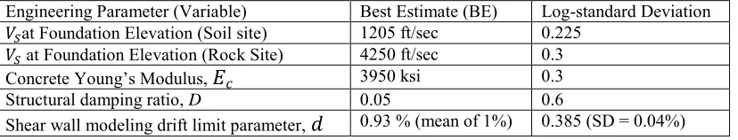
In the ISSFA analysis of the subject structure (of which, the nonlinear analysis presented here is a component), five parameters are identified for uncertainty modeling. These parameters are dynamic soil profile properties, young’s modulus for concrete ( ), structural damping ratio (
D
), and shear wallmodeling drift limit parameter, ( ). The mean and standard deviation corresponding to each of these parameters are provided in Table 3. For each parameter 30 realizations are simulated (randomized) assuming logarithmic-normal distribution for each, and randomly paired following Latin Hyper-cube Sampling (LHS) methodology as described in Hashemi et al. (2009). The uncertainty in the backbone curves is considered using a log-normal distribution for the drift limit parameter and assuming that other drift parameters and e are perfectly correlated with d and taken as 0.4d and 2.0d, respectively.
The uncertainty in the strength of each wall is considered through the uncertainty in (thus, uncertainty in ) for each wall. Therefore, the strength parameters f, and c are not further varied in the randomizations process. Figure 4 (b) presents the backbone curves for all 35 shear walls of the subject structure in the first realization of the LHS simulation. Through LHS, 30 realizations are generated for each one of the backbone curves for each wall. The randomized backbone curves for Wall 26 (2nd story-X direction on line 2) are presented as representative examples in Figure 4 (c).
Table 3. Input Parameters for Uncertainty Modeling
Engineering Parameter (Variable) Best Estimate (BE) Log-standard Deviation at Foundation Elevation (Soil site) 1205 ft/sec 0.225
at Foundation Elevation (Rock Site) 4250 ft/sec 0.3
Concrete Young’s Modulus, 3950 ksi 0.3
Structural damping ratio, D 0.05 0.6
Shear wall modeling drift limit parameter, 0.93 % (mean of 1%) 0.385 (SD = 0.04%)
SITE MODEL AND SITE RESPONSE ANALYSIS
In each of the rock and soil sites, the uncertainty in the subgrade profiles are represented through simulation (randomization) of 30 profiles given their respective best estimate profiles and their associated uncertainties. In each soil profile simulation, the uncertainty in the soil/rock shear wave velocity, damping ratio, layer thickness, and soil nonlinearity curves are taken into account. The site response analysis is conducted using the program SHAKE2000 (based on the work by Schnabel et al (1972)). Accordingly, the input time history for each run is applied as outcrop motion at top of the hard rock (VS≥9200 fps) and transmitted through the soil columns of the simulated profiles, therefore providing the acceleration time histories and strain-compatible profiles for each realization. The analysis is repeated at 3 hazard levels (1E-4, 1E-5 and 1E-6) and separately for LF and HF input motions (corresponding to HF4, HF5, HF6, LF4, LF5, and LF6 uniform hazard response spectra (UHRS)).
SSI ANALYSIS AND FOUNDATION MOTION DEVELOPMENT
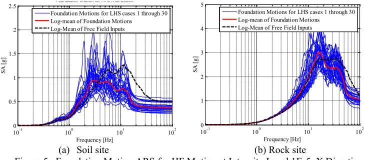
displacements). The nonlinear RHA applies the foundation acceleration time-histories in all directions simultaneously. The acceleration response spectra of the foundation motions obtained from the SSI analyses of the structure subjected to high frequency (HF) and low frequency (LF) motions at 1E-4, 1E-5, and 1E-6 hazard levels for both soil and rock subgrades are calculated. Figure 5 (a) and (b) provide a sample of these results for HF motions (30 realizations) at 1E-5 hazard level in the X direction for the soil site and the rock site, respectively. In the figures shown, the log-mean of the foundation acceleration response spectra (ARS) and the log-mean of the free-field surface ARS are also provided for comparison. It is observed that the SSI effects for the soil site subject to a horizontal HF input motion includes a significant shift in the frequency content of the input motion to the lower frequencies and reduction in the peak of the response spectra. For the rock site the SSI effects are generally much less significant when compared to the soil site case. Nevertheless, a shift toward lower frequencies is generally observed as well as amplification at the SSI frequency of the structure on rock (around 15 Hz in this case).
(a) Soil site (b) Rock site
Figure 5. Foundation Motion ARS for HF Motion at Intensity Level 1E-5, X Direction
NONLINEAR RESPONSE HISTORY ANALYSES AND RESULTS
The 3D nonlinear RHA are carried out using the nonlinear model described above in OpenSEES, using the foundation motion time-histories as input. The OpenSEES analysis is a time-domain analysis using Newmark integrator and mass and stiffness proportional damping defined in terms of structural frequency. Note that the value of the assigned nominal damping ratio varies in each of the 30 realizations of the structural model according to a log-normal distribution as defined in Table 3. The analysis time step is 0.005 sec. For each step the convergence test is carried out on the basis of the total energy corresponding to the unbalanced forces and displacements with a threshold of 10-8 kip-ft.
The nonlinear RHA results are obtained for runs (30 realizations for the HF and LF motions at 1E-4, 1E-5, and 1E-6 hazard levels on soil and on rock subgrades). The cases selected for presentation below are the 16th realization of the HF motion at 1E-6 hazard level (HF6) on the rock site and the 15th realization of the LF motion at 1E-6 hazard level (LF6) on the soil site. These cases exhibited the most severe nonlinear responses observed in the analysis of the structure. The force-deformation results presented here are for the major walls at column line 2 (X direction) shown in Figure 6.
10-1 100 101 102
0 0.5 1 1.5 2
2.5 Foundation Motion for HF5-X Direction
Frequency [Hz]
SA
[g
]
Foundation Motions for LHS cases 1 through 30 Log-mean of Foundation Motions
Log-Mean of Free Field Inputs
10-1 100 101 102
0 1 2 3 4
5 Foundation Motion for HF5-X Direction
Frequency [Hz]
SA
[g
]
Foundation Motions for LHS cases 1 through 30 Log-mean of Foundation Motions
(a) 16th Realization, HF, 1E-6 Hazard Level, Rock Site (b) 15th Realization, LF, 1E-6 Intensity Level, Soil Site
Figure 6. Examples of the Nonlinear Shear Wall Response (Column Line 2, X Direction)
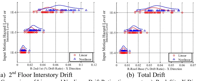
In the ISSFA analysis of the subject structure, the structural failure is defined in terms of the interstory drift ratio (differential displacement between the top and bottom of each story divided by the height of that story). These drift ratios are calculated both in linear analyses and nonlinear analyses at each input motion hazard level and for each LHS realization. Note that the results obtained at each hazard level are the envelope of HF and LF analysis results for that level (e.g. the 1E-4 maximum drift ratio is calculated as the envelope of the maximum drift ratio for the HF and LH 1E-4 runs). The rigid body rocking of the foundation is subtracted from the calculated drift ratios since the rocking component of the drift ratio does not contribute to the stresses in the shear walls or ultimately their failure. These results provide the drift ratio demand distribution at different ground motion hazard levels which are used to construct the shear wall fragility functions. The maximum absolute interstory drift ratios (between the 1st and 2nd floors in the X direction) and the total drift ratios (differential displacement between the roof and base mat divided by the building height) for the building are presented in Figure 7 and Figure 8 for the soil and rock subgrades, respectively. The drift ratios (in percentage) corresponding to the linear and nonlinear response for each LHS realization at each intensity level are shown by circular or triangular markers and their corresponding fits of a log-normal probability distribution functions are shown by the red and blue curves, respectively.
The results suggest that the nonlinearity in the structure (in X-direction) is likely to be limited to 2nd floor walls next to the openings. Accordingly, the 2nd floor drift obtained from the nonlinear analysis is up to 40% higher than the linear results. More significant structural nonlinearity is observed in the case of the structure supported on rock compared to soil subgrade. This is despite the fact that the total displacements observed in the soil case are more than twice those of the rock case. The reason is that the horizontal displacements calculated in the structure supported on soil are mainly due to foundation rocking and soil deformation rather than the structural deformations even at beyond design hazard levels 1E-5 and 1E-6. This suggests that when the structure is supported on soil subgrade the SSI effects (including soil nonlinearity) are much more dominant than the structural nonlinearity effects.
FE Model
Stick Model
-6 -4 -2 0 2 4 6 8 x 10⁻³
-6000 -4000 -2000 0 2000 4000 6000 8000 Element-1498 Displacement [ft] S he ar [k ]
-6 -4 -2 0 2 4 6 8 x 10⁻³
-1 -0.5 0 0.5 1 1.5
x 104 Element-1486
Displacement [ft]
Sh
ea
r [k
]
-0.02 -0.015 -0.01 -0.0050 0.0050.010.0150.020.025 -6000 -4000 -2000 0 2000 4000 6000 Element-1476 Displacement [ft] S he ar [k ]
-0.02 -0.01 0 0.01 0.02 0.03 -2500 -2000 -1500 -1000 -500 0 500 1000 1500 2000 2500 Element-1497 Displacement [ft] S he ar [k ]
-0.02 -0.015 -0.01 -0.00500.0050.010.0150.020.025 -1000 -500 0 500 1000 1500 Element-1502 Displacement [ft] S he ar [k ]
-6 -4 -2 0 2 4 6 8 x 10⁻³
-1.5 -1 -0.5 0 0.5 1
1.5x 10⁴ Element-1484
Displacement [ft] S he a r [k ] FE Model Stick Model
-3 -2 -1 0 1 2 3 x 10⁻³
-3000 -2000 -1000 0 1000 2000 3000 Element-1498 Displacement [ft] S h ea r [k ]
-4 -3 -2 -1 0 1 2 3 4 x 10⁻³
-6000 -4000 -2000 0 2000 4000 6000 Element-1486 Displacement [ft] S he ar [k ]
-4 -2 0 2 4 6
x 10-3
-4000 -3000 -2000 -1000 0 1000 2000 3000 4000 Element-1476 Displacement [ft] S he a r [k ]
-0.01 -0.005 0 0.005 0.01 0.015 -2000 -1500 -1000 -500 0 500 1000 1500 2000 2500 Element-1497 Displacement [ft] S he a r [k ]
-8 -6 -4 -2 0 2 4 6 8 x 10⁻³
-1000 -800 -600 -400 -200 0 200 400 600 800 1000 Element-1502 Displacement [ft] S he a r [k ]
-5 0 5
x 10-3
(a) 2nd Floor Interstory Drift (b) Total Drift
Figure 7. Comparison of Linear and Nonlinear Drift Ratios (in percentage), Soil Site, X Direction
(a) 2nd Floor Interstory Drift (b) Total Drift
Figure 8. Comparison of Linear and Nonlinear Drift Ratios (in percentage), Rock Site, X Direction
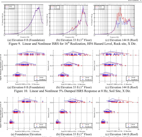
The failure of the non-structural components and safety related equipment in the structure is a function of the ISRS calculated at the location of that component. The ISRS are traditionally calculated from the linear analysis without consideration for structural nonlinearity. For the subject study, the ISRS are calculated at the intersection of major structural walls on Col. Line 2 and Col. Line B at Elevations 0 ft (foundation), 33 ft (1st floor) and 144 ft (roof). The ISRS at these nodes in the model are calculated from both linear and nonlinear analysis results. As an example, the comparison between the 5% damped ISRS obtained from the linear and nonlinear models for the 16th realization of the HF motion at 1E-6 intensity level on the rock site are shown in Figure 9. Note that the ISRS calculated on the foundation are of course identical in both cases, while small differences are observed in the ISRS calculated at Elevation 33 ft. However, the roof ISRS calculated from the nonlinear case is significantly lower than that obtained from the linear analysis. This observation is consistent with the nonlinear response of the structure (see Figure 6 (a)) which shows significant nonlinear response above Elevation 33 ft. The reduction in the ISRS is attributed to the additional hysteresis damping as well as instantaneous frequency shifts due to softening of the structure. Finally, the value of the ISRS at 8 Hz (corresponding to the natural frequency of a supposed important-to-safety equipment) are calculated using ISRS from linear and nonlinear analysis for each intensity level and for soil and rock cases and presented in Figure 10 and Figure 11, respectively. Similar to earlier observations, as the hazard levels increase, the structure experiences more nonlinear deformation, and more hysteresis damping dissipated in the structure which result in a reduction in the ISRS response at 8 Hz. These reductions in some instances are very significant, as observed in the rock case at 1E-6 hazard level, and may have large impact on the resulting fragility analyses. Also note that while a reduction in the ISRS due to structural nonlinearity is expected, for most practitioners the complexity of the nonlinear analysis is prohibitive and they choose to use the ISRS from the linear analysis for design purposes.
0 0.02 0.04 0.06 0.08 0.1
1E-4 1E-5 1E-6
R-2nd-1st (% Drift Ratio) - X Direction
In
te
ns
ity
L
ev
el
Case-5N-LR and Case-5N-LR-001 Results
Linear Nonlinear
0 0.01 0.02 0.03 0.04 0.05 0.06 1E-4
1E-5 1E-6
R-Roof-Base (% Drift Ratio) - X Direction
In
te
ns
ity
L
ev
el
Case-5N-LR and Case-5N-LR-001 Results
Linear Nonlinear
0 0.02 0.04 0.06 0.08 0.1 0.12 1E-4
1E-5 1E-6
R-2nd-1st (% Drift Ratio) - X Direction
In
te
ns
ity
L
ev
el
Case-6N-LR and Case-6N-LR-001 Results
Linear Nonlinear
0 0.01 0.02 0.03 0.04 0.05 0.06 0.07 1E-4
1E-5 1E-6
R-Roof-Base (% Drift Ratio) - X Direction
In
te
ns
ity
L
ev
el
Case-6N-LR and Case-6N-LR-001 Results
Linear Nonlinear
Inp
ut
M
otio
n
H
az
ar
d
Le
ve
l or
Inp
ut
M
otio
n
H
az
ar
d
Le
ve
l or
Inp
ut
M
otio
n
H
az
ar
d
Le
ve
l or
Inp
ut
M
otio
n
H
az
ar
d
Le
ve
(a) Elevation 0 ft (Foundation) (b) Elevation 33 ft (1st Floor) (c) Elevation 144 ft (Roof)
Figure 9. Linear and Nonlinear ISRS for 16th Realization, HF6 Hazard Level, Rock site, X Dir.
(a) Elevation 0 ft (Foundation) (b) Elevation 33 ft (1st Floor) (c) Elevation 144 ft (Roof)
Figure 10. Linear and Nonlinear 5% Damped ISRS Response at 8 Hz, Soil Site, X Dir.
(a) Foundation Elevation (b) Elevation 33 ft (1st Floor) (c) Elevation 144 ft (Roof)
Figure 11. Linear and Nonlinear 5% Damped ISRS Response at 8 Hz, Rock Site, X Dir.
CONCLUSIONS
Important observations from the nonlinear analysis of the subject structure including SSI effects are summarized below:
The results of nonlinear analysis of the structure pointed to more significant structural nonlinearity in the case of the structure supported on rock compared to soil subgrade. This is despite the fact that the total displacements observed in the soil case are more than twice those of the rock case. The reason is that the horizontal displacements calculated in the structure supported on soil are mainly due to foundation rocking and soil deformation rather than the structural deformations even at beyond design hazard levels 1E-5 and 1E-6. This suggests that when the structure is supported on soil subgrade the SSI effects (including soil nonlinearity) are much more dominant than the structural nonlinearity effects.
The ratio of the nonlinear to linear total drift for the considered structure can be reasonably taken as
unity. This corroborates the widely used assumption that the linear and nonlinear total displacements 100-1 100 101 102
1 2 3 4 5 6 7 8 Frequency [Hz] 5% D am pe d A RS [g ]
Linear and Nonlinear Comparison of ISRS, HF6, LHC-16, Node 426- X Linear
Nonlinear
Linear: X:\Alidad\StickModel\Case_6N_LR_001 Nonlinear: X:\Alidad\StickModel\Case_6N_LR Sliding: X:\Alidad\StickModel\Case_6N_LR_NLSliding
10-1 100 101 102
0 2 4 6 8 10 12 14 Frequency [Hz] 5% D am pe d A RS [g ]
Linear and Nonlinear Comparison of ISRS, HF6, LHC-16, Node 785- X Linear
Nonlinear
Linear: X:\Alidad\StickModel\Case_6N_LR_001 Nonlinear: X:\Alidad\StickModel\Case_6N_LR Sliding: X:\Alidad\StickModel\Case_6N_LR_NLSliding
10-1 100 101 102
0 2 4 6 8 10 12 14 Frequency [Hz] 5% D am pe d A RS [g ]
Linear and Nonlinear Comparison of ISRS, HF6, LHC-16, Node 2472- X Linear
Nonlinear
Linear: X:\Alidad\StickModel\Case_6N_LR_001 Nonlinear: X:\Alidad\StickModel\Case_6N_LR Sliding: X:\Alidad\StickModel\Case_6N_LR_NLSliding
0 0.5 1 1.5 2
1E-4 1E-5 1E-6
Node426 ISRS at 8 Hz - X Direction
In te ns ity L ev el
ISRS Results at 8 Hz
Linear Nonlinear
0 0.5 1 1.5 2
1E-4 1E-5 1E-6
Node785 ISRS at 8 Hz - X Direction
In te ns ity L ev el
ISRS Results at 8 Hz
Linear Nonlinear
0 1 2 3 4 5 6 7 1E-4
1E-5 1E-6
Node2472 ISRS at 8 Hz - X Direction
In te ns ity L ev el
ISRS Results at 8 Hz
Linear Nonlinear
0 1 2 3 4 5 6 7 1E-4
1E-5 1E-6
Node426 ISRS at 8 Hz - X Direction
In te ns ity L ev el
ISRS Results at 8 Hz
Linear Nonlinear
0 1 2 3 4 5 6 7 1E-4
1E-5 1E-6
Node785 ISRS at 8 Hz - X Direction
In te ns ity L ev el
ISRS Results at 8 Hz
Linear Nonlinear
0 5 10 15 20
1E-4 1E-5 1E-6
Node2472 ISRS at 8 Hz - X Direction
In te ns ity L ev el
ISRS Results at 8 Hz
are equal. However, locally (i.e. 2nd floor drift in the example structure), the nonlinear drift ratios may be significantly larger than the linear drift ratios due to concentration of the shear wall deformations at a single (weak story) level.
The additional hysteresis energy dissipated in the structure and instantaneous shift in the structural frequency due to the nonlinear response of the structure has the potential to significantly reduce the ISRS (especially its peak) above the elevations at which nonlinearity occurs. For the subject structure, these reductions are very significant for the rock subgrade case at higher hazard levels.
For both soil and rock supported structures the drift ratios calculated at design and beyond design levels are much smaller than the specified drift ratio capacity of the shear walls (estimated as 0.5% on average). This reflects the robustness of the structure and is typical of this type of construction for nuclear buildings where a larger component of the overall failure risk is due to non-structural components and equipment rather than structural components. The seismic demands on such components are obtained from the ISRS results. The fragility calculation and performance of both structural and non-structural components and equipment are provided as part of the ISSFA analysis and will be discussed in future publications.
REFERENCES
American Society of Civil Engineers (2007). Seismic Rehabilitation of Existing Buildings (ASCE 41-06 and Supplement-1), ASCE, Reston, Virginia, USA.
American Society of Civil Engineers (2005). Seismic Design Criteria for Structures, Systems, and Components in Nuclear Facilities (ASCE 43-05), ASCE, Reston, Virginia, USA.
Elkhoraibi TE and Hashemi, A. (2012). Design Applications for Integrated Soil-Structure Fragility Analysis. Bechtel Technical Grant Report.
Elkhoraibi, T.E. and Hashemi, A. (2011). “Integrated Soil-Structure Fragility Analysis Method for Nuclear
Structures,”. Fifth International Conference on Earthquake Geotechnical Engineering. Santiago, Chile, 10–13 January 2011.
Hashemi, A., Elkhoraibi, T.E., and Ostadan, F. (2012), “Probabilistic Nonlinear Analysis of a RC Shear Wall Structure including Soil-Structure Interaction,” 15th World Conference on Earthquake Engineering (15WCEE), Lisbon, Portugal, 24-28 September 2012.
Hashemi, A., Elkhoraibi, T.E., and Ostadan, F. (2011). Probabilistic and Deterministic Soil Structure Interaction (SSI) Analysis. Eleventh International Conference on Application of Statistics and Probability in Civil Engineering (ICASP11), ETH Zurich, Switzerland, 1–4 August 2011.
Hashemi, A. and Elkhoraibi, T.E. (2009). “Integrated Soil-Structure Fragility Analysis Method,” ECCOMAS Thematic Conference on Computational Methods in Structural Dynamics and Earthquake Engineering (COMPDYN 2009), Rhodes, Greece, 22–24 June 2009.
Mazzoni, S., McKenna, F., Scott, M.H., Fenves, G.L., et al. (2006). Open System for Earthquake Engineering Simulation User Command-Language Manual. Pacific Earthquake Engineering Research Center, University of California, Berkeley, OpenSees version 1.7.3.
Schnabel, P.B., Lysmer, J. and Seed, H.B. (1972). “SHAKE: A Computer Program for Earthquake Response Analysis of Horizontally Layered Sites,” Report No. USB/EERC-72/12, Earthquake Engineering Research Center, University of California, Berkeley, December.
University of California at Berkeley (2011). SASSI2010 - A System for Analysis of Soil-Structure Interaction. Bechtel Standard Computer Program (SCP), GE996 Version 1.0., November 2011.