ABSTRACT
CHEN, XIAOMEI. Discounting Investments that Save Energy Resources. (Under the direction of Michael Roberts and Laura Taylor.)
In the first chapter, I focus on the relationship between energy futures and the aggregate economy. Wide and frequent variation in the association between energy futures and the overall stock market facilitates a novel test of the conditional Capital Asset Pricing Model (CAPM). Using commodity futures and covariances with the S&P 500, I find excess returns on rollover futures contracts to be strongly associated with market betas, and fail to reject conditional CAPM when weekly beta estimates are corrected for measurement error. Moreover, the time path of estimated betas of crude oil reflects historical shocks to demand and supply that would naturally give rise to betas of different signs. Examples include the Gulf War of 1990-1991 (negative beta), Iraq War of 2003 (negative beta), OPEC oil expansion in 1986 (negative beta), and Recessions of 2000 and 2007(positive betas).
In the second chapter, I examine how uncertainty affects the choice of discount rate especially in the context of energy investments. The expected present value of investments that pay dividends in the form of energy savings is strongly influenced by uncertainty about discount rates. Discount rate uncertainty stems from interest rate uncertainty, risk premium uncertainty and energy-price uncertainty. I develop a state-space model that simultaneously considers all three components of the discount rate and use the model to project uncertainties into the future. From these projections, I estimate certainty-equivalent discount rates for investments with different longevities, including fuel efficient cars (10-15 years), photovoltaic solar panels and windmills (20-30 years). I find certainty-equivalent discount rates are sensitive to model specification but tend to be much lower than discount rates conventionally used in practice.
© Copyright 2013 by Xiaomei Chen
Discounting Investments that Save Energy Resources
by Xiaomei Chen
A dissertation submitted to the Graduate Faculty of North Carolina State University
in partial fulfillment of the requirements for the Degree of
Doctor of Philosophy
Economics
Raleigh, North Carolina
2013
APPROVED BY:
Michael Roberts
Co-chair of Advisory Committee
Laura Taylor
Co-chair of Advisory Committee
Walter Thurman Denis Pelletier
DEDICATION
BIOGRAPHY
ACKNOWLEDGEMENTS
TABLE OF CONTENTS
LIST OF TABLES . . . vi
LIST OF FIGURES . . . vii
CHAPTER 1 A Test of Conditional CAPM using High Frequency Energy Futures Prices . . . 1
1.1 Introduction . . . 1
1.2 Methods . . . 4
1.2.1 Testing the Short-Window CAPM . . . 6
1.2.2 Error-in-variable Corrections . . . 6
1.3 Data . . . 9
1.4 Testing with crude oil futures . . . 11
1.5 Testing other Energy Resources . . . 20
1.6 Conclusion . . . 31
CHAPTER 2 Discounting Investments that Save Energy Resources. . . 32
2.1 Introduction . . . 32
2.2 A Simple Numerical Example . . . 35
2.3 Estimating Risk Premium using the Capital Asset Pricing Model . . . 37
2.4 Vector Autoregressive Models . . . 41
2.5 Fuel consumption estimation . . . 42
2.6 Path-wise Simulations forβt,rt,rMt ,Pt and Qst . . . 42
2.7 Data and Estimation Results . . . 43
2.8 Discussion . . . 64
2.9 Appendix . . . 67
CHAPTER 3 Can Standards Increase Consumer Welfare? Evidence from a Change in Clothes Washer Energy Efficiency Requirements. . . 72
3.1 Introduction . . . 72
3.2 Consumer Welfare Analysis of a Change in Standards . . . 73
3.3 Assessing the Value of Washer Attributes . . . 78
3.4 Data and its Limitations . . . 79
3.5 Price and Quantity Changes Over Time . . . 85
3.6 Regression Models . . . 85
3.7 Minimum Change in Consumers’ Surplus . . . 93
3.8 Discussion . . . 94
3.9 Appendix . . . 98
3.9.1 Analysis of 2004 Policy Change . . . 98
LIST OF TABLES
Table 1.1 Commodity Trading Information . . . 10
Table 1.2 Conditional Betas for Crude Oil Futures of Different Sample Periods . . . 11
Table 1.3 CAPM Results - Summary . . . 18
Table 1.4 Simulation Extrapolation Results using Different Fitting Methods . . . 19
Table 1.5 Summary of Pricing Error (%) . . . 20
Table 1.6 Summary of Market Betas . . . 22
Table 1.7 CAPM Results - Summary . . . 29
Table 1.8 SIMEX results for Energy Commodities . . . 30
Table 2.1 The Annualized Constant Equivalent Discount Rate (%) for Projects with 10 Years Lifetime . . . 56
Table 2.2 The Annualized Constant Equivalent Discount Rate (%) for Projects with Different Lifetimes . . . 61
Table 2.3 The Annualized Constant Equivalent Discount Rate for Simulations using Different Starting Points . . . 63
Table 2.4 Start Values for Each Point in Time . . . 64
Table 2.5 The Annualized Equivalent Discount Rate (%) for Projects with 25 Years Lifetime . . . 69
Table 2.6 The Annualized Equivalent Discount Rate (%) for Projects with 50 Years Lifetime . . . 70
Table 2.7 Annualized Constant Equivalent Discount Rate (%) for Projects with Dif-ferent Lifetimes . . . 71
Table 3.1 Summary Statistics of the Full Sample . . . 81
Table 3.2 Summary Statistics of the Limited Sample . . . 83
Table 3.3 Summary of Regressions . . . 93
Table 3.4 Estimates of Minimum Change in Consumer Surplus . . . 95
Table 3.5 Summary Statistics of the Limited Sample . . . 99
LIST OF FIGURES
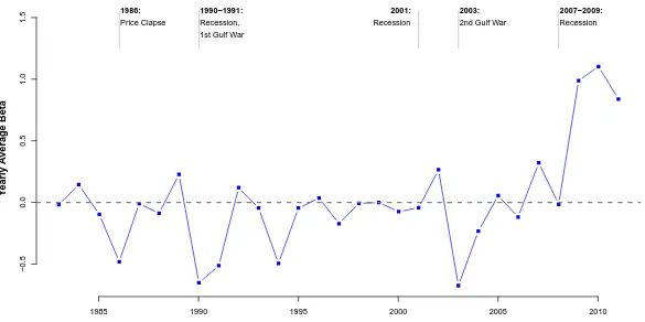
Figure 1.1 Yearly Average Beta and Events of the year . . . 13
Figure 1.2 Performance of CL and S&P 500 in relation to Beta . . . 15
Figure 1.3 SIMEX with Different Fitting Methods . . . 17
Figure 1.4 T-values of Estimated Pricing Error . . . 21
Figure 1.5 T-values of Estimated Market Betas . . . 23
Figure 1.6 Performance of all Commodity Futures and S&P 500 . . . 25
Figure 1.7 Performance of Energy Commodities and their betas . . . 27
Figure 1.8 Risk Premium (% per 2-week period) . . . 28
Figure 2.1 Filtered Beta (AR(1)) with 90% Confidence Interval . . . 46
Figure 2.2 The CAPM predicted risk premium (%/bi-week) . . . 48
Figure 2.3 Simulated predictions of beta over the next 5 years . . . 50
Figure 2.4 Simulated predictions of oil price over the next 5 years . . . 51
Figure 2.5 Simulated predictions of energy savings over the next 5 years . . . 52
Figure 2.6 Simulated predictions of market return over the next 5 years . . . 53
Figure 2.7 Simulated predictions of risk free return over the next 5 years . . . 54
Figure 2.8 Annualized Constant equivalent Discount Rate (%) . . . 58
Figure 2.9 Constant-Equivalent Discount Rate by Elasticity of Demand . . . 60
Figure 2.10 Filtered Beta (Random Walk) with 90% Confidence Interval . . . 68
Figure 3.1 The standard change reduces supply of low-efficiency units. . . 75
Figure 3.2 The standard change shifts out demand for high-efficiency units. . . 76
Figure 3.3 Washer Units Sold — Full Sample . . . 86
Figure 3.4 Washer Units Sold — Limited Sample (models existed before and after 2007) . . . 87
Figure 3.5 Average Washer Prices — Full Sample . . . 88
Figure 3.6 Average Washer Prices — Limited Sample (models existed before and after 2007) . . . 89
Figure 3.7 Market Share — Full Sample . . . 90
Figure 3.8 Market Share — Limited Sample (models existed before and after 2007) . 91 Figure 3.9 Washer Units Sold — Limited Sample (models existed before and after 2004) . . . 102
Chapter 1
A Test of Conditional CAPM using
High Frequency Energy Futures
Prices
1.1
Introduction
The Capital Asset Pricing Model (CAPM) is the benchmark theory for how markets incorporate risk into asset prices. The theory shows that an asset’sbeta connects asset-specific risk premia to the economy-wide market risk premium.Beta measures the association of an asset with the market portfolio. The higher an asset’s beta, the less of its risk can be diversified away, and thus the higher its risk premium.
While the theory remains a standard part of economics and business school training, empir-ical evidence in support of the theory remains varied and inconclusive. Early empirempir-ical efforts failed to reject the theory, but these tests lacked statistical power, in part because most equi-ties covary together. Without large differences in predicted risk premia, stocks give little basis for comparison. Earlier analysis of cross-sectional data finds a relationship between realized returns and estimated market beta that is too flat relative to CAPM predictions (Black, Jensen and Scholes 1972, Blume and Friend 1973, Fama and MacBeth 1973, and many others). Later work by Fama and French (1992, 1996) devastated CAPM by showing betas explained none of the predictable differences in returns across portfolios sorted by firm size and book-to-market ratios, the largest and most persistent predictable differences in stock returns that have been identified.
book-to-market ratios have large betas during recessions when market risk premia are large, and small betas during booms when market risk premia are small. For large companies and “growth” stocks with low book-to-market ratios, the opposite pattern emerges. These relation-ships show how CAPM can reconcile the relatively higher average returns of small company stocks and value stocks as compared to stocks of large companies and growth stocks. More recently, Lewellen and Nagel (2006) challenged these findings by arguing it would require betas to vary by an implausible amount.
In this paper we consider a general conditional CAPM model in the context of commodity market returns, rather than stocks. Commodity markets provide a particularly interesting area to test the predictions of CAPM because commodity prices do not generally covary systemati-cally with each other or with stocks (Bodie and Rosansky, 1980). That is, different commodities have very different betas, facilitating a larger scope for comparison and greater statistical power. Commodity betas are also likely to vary over time for clear fundamental reasons that may or may not be related to business cycles. For example, an unexpected discovery of a large new oil deposit would presumably cause oil prices to decline while simultaneously providing good news for the aggregate economy and stock returns. Such an event would be embodied by a negative
beta and risk premium under CAPM. Conversely, larger-than-expected growth in emerging markets may drive up demand of both stocks and oil prices, giving rise to a positive beta. Precious metals like gold may also be used as a hedge against inflation or financial crises, and thus may have varying and possibly even negative risk premiums. For these reasons, commodity markets provide a wholly different and powerful area for testing CAPM.
In this study, we focus on energy products — crude oil, natural gas, heating oil and gasoline — which are important industrial commodities closely related to the overall economy that have been traded in futures markets for many decades. The well-documented connections between the energy market and the macroeconomy also make these commodities interesting when testing CAPM (Hamilton 1983, Barsky and Kilian 2004, Kilian 2009). This literature indicates that through much of post-World-War II history, supply shocks or anticipated supply shocks have been a major source of the price volatility, particularly for oil. These shocks have mainly followed from conflicts in the Middle East, actions taken the Organization of Petroleum Exporting Countries (OPEC), and discovery of major new oil deposits. These shocks likely played at least a contributing role in many post World War II recessions and often gave rise to a negative association between energy price changes and overall market, hence negative average betas. At other times, and especially recently, energy price changes have been associated with aggregate demand shocks following from global booms, recession and recovery, likely giving rise to positive betas.
experienced large aggregate demand shocks following the 2008 financial crisis, likely giving rise to positive betas. At the same time, however, civil conflict in Libya and parts of the Middle East gave rise to supply shocks and fear of even larger future supply shocks, which could create negative betas. It is therefore easy to see how beta size and sign could change considerably, perhaps even from one week to the next, depending on which kind of events were perceived by the market to be more prevalent.
It requires little introspection to see that, for all assets, betas may change over time quite ar-bitrarily. Similarly, the risk premium for the market-portfolio may change over time, depending upon perceived uncertainty about aggregate economic growth. The basic asset pricing theory provides no guidance about the structure of these deeper sources of time-varying variances and covariances. More challenging still is that changing expectations about market returns and asset-specific covariances, including the examples for energy-specific assets described above, are unlikely to be quantifiable using objective measures or factors. For this reason, Cochrane (2001) (with attribution to Hansen and Richard (1987)) argues that CAPM, in its most generic form, is fundamentally untestable.
Without some structure to pin down clear comparisons between relatively low-risk-premium assets and high-risk-premium assets, there is little defensible scope for testing the theory. A statistical rejection CAPM may result because the econometrician has assumed conditioning information or some structure that causes assets to have been assigned to incorrect betas and/or risk premiums.
The key contribution of this analysis is to provide a simple structure for time-varying betas that does not assume betas are fixed over time (Dusak 1973; Bodie and Rosansky 1980) or require factor variables to account for changing conditional expectations (Merton 1973, Bree-den 1979, Cox, Ingersoll Jr and Ross 1985 among others). Instead of using conditioning factors (which are likely unmeasureable in most cases), we estimate betas using short-window regres-sions that follow in the spirit of Lewellen and Nagel (2006). We also consider a model that assumes a latent stochastic structure for an underlying beta process, which we are able to estimate using a Kalman filter.
To allow betas to change at a high frequency, we use an approach developed by Lewellen and Nagel (2006) and directly estimate betas and risk premia unconditionally through short-window regressions. This approach is simple and requires fewer structural assumptions than earlier empirical tests of conditional CAPM (Jagannathan and Wang 1996, Lettau and Ludvigson 2001 etc.). Using daily returns in the estimating of the short-window regressions, we use a 2-week period as a baseline window size.
current-period beta; (2) a Kalman filter assuming the underlying true beta follows a random walk; and (3) using simulation extrapolation (SIMEX) (Cook and Stefanski 1994). SIMEX is simulation based technique that adds a series of additional error vectors to the observed data, with each vector series having a different variance. The series of coefficient estimates are then used to extrapolate what the estimate would be if there were no error in the estimated beta; and the results are asymptotically unbiased and consistent (Cook and Stefanski 1994).
The results show considerable variations in estimated betas over time for all energy com-modities. Crude oil betas, for example, have a mean of 0.01 and standard deviation of 1.1. An estimated 62% of the beta variance is due to measurement error, and 38% due to true variation in betas. Crude oil and petroleum products such as gasoline and heating oil are correlated with oil but have slightly different betas.
We find realized return premiums vary significantly with estimated betas over time and across commodities. Where most earlier tests find realized premiums to be smaller than CAPM-estimated premiums, we find realized return premiums increase somewhat more than one for one with estimated premiums.
We test the short-window CAPM by examining (1) the statistical properties of estimated bi-weekly pricing error, alpha, and the risk index, beta; (2) the economic interpretation of the estimated beta; and (3) the comparison between the realized risk premiums and its CAPM predicted counterparts over time. In (1) the pricing error is the deviation of the realized risk premium from its CAPM prediction which can be captured by the intercept in the short-window regressions. The CPAM predicted risk premium can be calculated using the estimated beta, and (3) can be achieved by regressing actual returns on the calculated ones.
1.2
Methods
To test CAPM for commodity trading, we consider speculative trading of commodity futures. Commodity futures are a natural setting for testing CAPM because investors can speculate and trade in these markets with minimal transactions costs and without physically holding or storing the commodity. Specifically, we consider buying and subsequently selling of futures contacts. Contracts are always sold at least 1 week before the final trading date such that the speculator need not ever take physical possession of the commodity. Contracts for the nearest delivery date are bought and sold up to one week before the last trading day, at which time contracts are rolled over to the subsequent delivery date. Arbitrage pricing rules apply to these derivative contracts, and via arbitrage the associated risk premia ought to apply equally to the physical commodities.
return in periodt for holding the futures contract from periodt−1 to periodt is therefore:
rt=ln(F(t, Td))−ln(F(t−1, Td))
In practice, to buy a futures contract, the buyer must post a Treasury bill as collateral for funds promised on the delivery date. The return on the Treasury bill must therefore be added tort. And the daily commodity realized return is:
Rt=rt+Rft
and Rft is the treasury return. We use 3-month t-bill as the risk-free asset, and its daily return is calculated following standard Treasury bill return calculation and formula is specified as follows:
Rf =
1
1−rf ·(91/360)
(days/91)
−1
where rf is the 3-month Treasury bill rate, calculated as the daily secondary market quote
on the most recently auctioned Treasury Bills for 3-month maturity. In case of missing rate, the rate of the nearest neighbor prior will be used. The variabledays refers to the number of calendar days investor holds the risk-free asset. This equation follows the formula used in “The Dow Jones-UBS Commodity IndexSM Handbook” for calculating 3-month t-bill return.
We use S&P 500 as the proxy to the overall-market, and its daily return is defined as:
RMt =ln(PM t+DM t)−ln(PM t−1)
whereDM t is the daily dividend calculated from the reported quarterly dividend.
The asset risk premium is defined as the excess return in excess of the risk-free return. Accordingly, the risk premium in the futures market is
rt=Rt−Rft
=ln(F(t, Td))−ln(F(t−1, Td))
Whereas the market risk premium is
rtM =RMt −Rft
each commodity and each 2-week period
rt,τi =αiτ+βiτrt,τM +it,τ (1.1)
t= 1,· · ·,10
where ri
t,τ and rMt,τ are the realized risk premium on commodity i and the market portfolio
respectively of the 2-week period τ. αiτ is the deviation of realized risk premium from the
CAPM prediction, or the pricing error. And βiτ represents the exposure of asset i to market risk in the 2-week periodτ.
1.2.1 Testing the Short-Window CAPM
The time series of ατ and βτ we obtain from estimating equation 1.1 enable several different tests of CAPM. The most straightforward ways are testing whether pricing error, α, is zero, and whether the market risk coefficient, β, reflects the true risk premia.
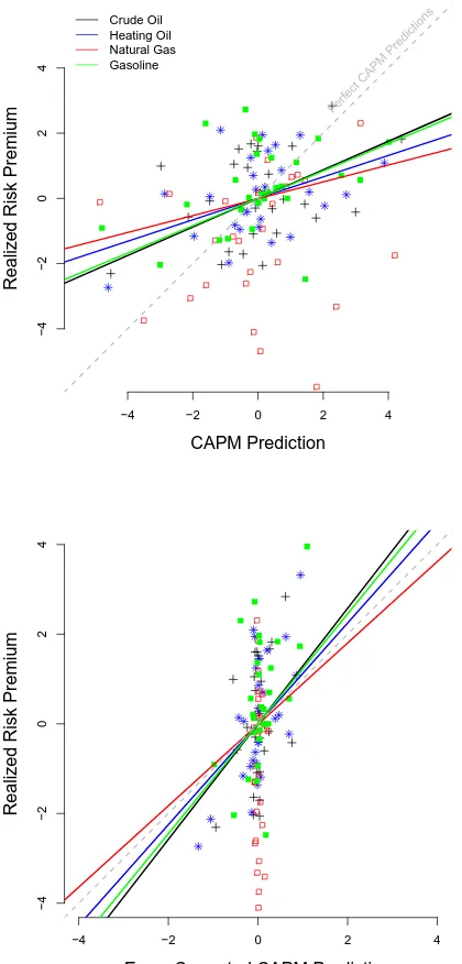
Further, by comparing the realized risk premiums to the CAPM predictions, which equal to the market risk premiums multiplied bybeta, we can understand how accurately the model predicts over time. This test can be achieved through a simple regression using estimated bi-weekly betas and realized market and asset-specific risk premiums over time for each of the commodities:
riτ =δ0+δ1( ˆβiτrτM) +µiτ (1.2)
where ˆβiτ is the estimated beta of asset ias of 2-week period τ. riτ and rτM are bi-weekly risk
premiums of asseti and market portfolio respectively.
If CAPM predicts the risk premium, the realized risk premium equals its CAPM prediction, i.e.riτ = ˆβiτrτM, plus a pricing error. It gives us testable hypotheses thatδ0 = 0 andδ1 = 1.
1.2.2 Error-in-variable Corrections
Bi-weekly betas are estimated in the previous step using small sample sizes, which leads to large estimation error and causes an attenuation bias when they are used directly in estimating equation 1.2. In this section, we propose three ways to correct for the bias: (1) use of an instrumental variable, (2) Kalman filter, and (3) simulation extrapolation.
then exclusionary assumptions are satisfied and instrument has a strong foundation. In the first stage we estimate model 1.2:
ˆ
βiτ =φ0+φ1βˆiτ−1+νiτ−1 (1.3)
We then use the fitted values of beta in equation 1.3 for the estimation of model 1.2 in the second stage.
In another attempt to correct for the estimation error, we use the Kalman filter in the state space model. The state space model is a flexible form that can be formulated to model dynamic time series with measurement error. A local level model is used in this study, and the state space representation of short-window betas can be written as:
ˆ
βt=βt+υt (1.4)
βt=βt−1+ωt (1.5)
whereυt∼N(0, V) and ωt∼N(0, W).
Equation 1.4 states that the ˆβtestimated using the short window regressions is composed of the truebeta,βt, and the estimation error,t. Equation 1.5 assumes that the truebeta follows a
random walk. This purpose of this method is to infer relevant properties of the unobserved true
β from the observations of ˆβ. We modify the model derivation in Harvey, Ruiz and Sentana (1992) and Kim and Nelson (1999), use Kalman Filter recursions to filter out the error term in Equation 1.4, and get the series of underlying true beta through the process. Detailed model modifications and derivation process can be found in Chapter 2.
In the first two methods, we correct for the bias using some econometric assumptions of the time series properties ofbetas. In this part, we introduce a statistical technique, Simulation extrapolation (SIMEX), which is simulation based without making assumptions onbeta. SIMEX is an error correction technique developed by Cook and Stefanski (1994), where by estimating the regressions with additional errors added, we can establish a trend between estimates and variances of additional error and then extrapolate back to where there is no error. SIMEX works well when measurement error is known or can be well approximated, and since betas are estimated using short-window regressions, we have the estimation error for each estimated
beta and use the arithmetic average of these errors as a proxy of the measurement error. The relationship between the estimated beta and the true beta is as follows:
ˆ
βτ =βτ +σZτ (1.6)
And we use the following step of SIMEX to correct for this error.
1. Add pseudo errors to the estimated betas
¯
βτ = ˆβτ+λ1/2σZτ (1.7)
whereλis chosen with known increment.
2. Estimate regressions using the constructed betas
riτ =δλ0 +δλ1( ¯βτrτM) +µiτ (1.8)
For each chosen λ, we draw N random numbers from the standard normal distribution,
Z. After estimating Equation 1.8 for each Z, we take the arithmetic average of all N estimated δZ0 and δ1Z. We then get the paired λand δ.
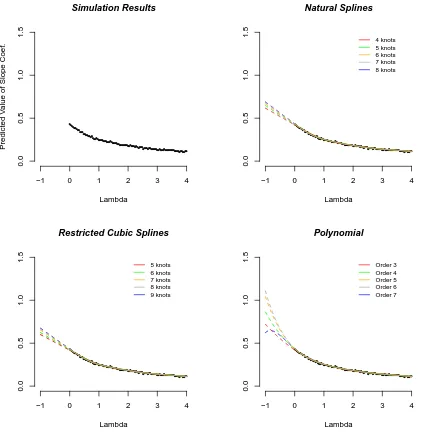
3. Establish the trend between the estimated average δ0 and δ1 with λ. We use different fitting methods for comparison purposes, namely restricted cubic splines, natural splines and polynomial.
4. Extrapolate the trend to where there is no error.
We show as follows that the constructed ¯β has the mean of the true beta in Equation 1.9; and its variance can be reduced to the variance of the true beta when λ=−1 in Equa-tion 1.10.
E( ¯βτ) = E( ˆβτ) +λ1/2σE(Zτ) = E(βτ+σZτ)
= E(βτ) (1.9)
V ar( ¯βτ) = V ar( ˆβτ) +λσ2V ar(Zτ) = V ar(βτ+σZτ) +λσ2
= V ar(βτ) +σ2+λσ2 (1.10)
1.3
Data
Futures contracts have different delivery months, and we choose to hold only the nearest con-tracts and roll concon-tracts into the next contract one week before the last trading day. For ex-ample: in September, we hold the crude oil futures contracts that deliver in October, and roll the October contracts into the November contracts one week before the last trading day of the October contract, usually around 15th of the month. Our futures data is from the Commod-ity Research Bureau (CRB), which covers all commodCommod-ity futures with daily prices (including “Open”, “High”, “Low”, and “Settle”) and volume series (including “Open Interest” and “Vol-ume”) for most contracts. We choose the daily “Settle” prices to get daily returns for all the commodities in the study.
Table 1.1 includes the start and end dates of the daily futures price series, and the trading information of each commodity we study in the paper. These futures all have monthly delivery and are traded heavily in the New York Mercantile Exchange, Inc. (NYMEX).
Table 1.1: Commodity Trading Information
Commodity Code Last Trading Day Start End
Light, Sweet Crude Oil CL The third business day prior to the 25th calendar 3/30/1983 12/16/2011 day of the month preceding the contract month.
Heating Oil HO The last business day of the month 11/14/1978 12/16/2011
preceding the contract month.
Henry Hub Natural Gas NG The third business day prior to 4/4/1990 12/16/2011
the first calendar day of the contract month. Gasoline Blendstock
RB The last business day of the month 1/1/1985 12/16/2011
New York Harbor preceding the contract month.
Note:
1. All commodities are traded in NYMEX
Table 1.2: Conditional Betas for Crude Oil Futures of Different Sample Periods
(1983/04- (1983/04- (1990/06- (1997/08- (2004/10-2011/12) 1990/05) 1997/07) 2004/9) 2011/12)
Observations 750 187 187 188 188
Minimum -8.11 -6.17 -8.11 -4.11 -2.94
25% -0.47 -0.30 -0.92 -0.56 -0.18
Median 0.03 -0.00 -0.16 -0.03 0.47
Mean 0.01 -0.05 -0.24 -0.10 0.42
75% 0.60 0.30 0.51 0.41 0.98
Maximum 6.79 2.87 5.15 2.81 6.79
Std Deviation 1.14 0.92 1.39 0.95 1.15 Skewness -0.59 -2.24 -0.83 -0.72 0.79
Kurtosis 7.59 14.54 6.44 2.63 4.68
1.4
Testing with crude oil futures
Historical crude oil prices have fluctuated with shifts in worldwide demand and supply. The real price fell mostly from 1870-1970 in response to discoveries of oil deposits, then rose sharply in 1970s due to conflicts in the Middle East such as the Yom Kippur war and Iranian revolutions. Prices fluctuated a lot during the 80s and 90s, responding to the combination of the effects of global recessions and Middle East conflicts, before it rose steadily due to the high demand induced by strong growth in the emerging markets. A considerable literature (Kilian 2008) shows oil prices have been associated with the overall economy, and we further document and help to clarify these links in this paper using the CAPM.
Another issue also worth noting is that beta becomes positive on average over the more recent decade, which can be attributed to a combination of fast economic growth in Asia, and the recent global recessions. Much of the huge variations in estimated betas, ranging from -8.11 to 6.79, are likely due to large sampling error. But large variations in the true but unobservable betas are supported by the frequent changes in demand and supply shocks, and the time path of betas seems broadly consistent with historical events.
1985 1990 1995 2000 2005 2010
Y
earl
y A
vera
g
e Beta
−0.5
0.0
0.5
1.0
1.5
1986:
Price Clapse
1990−1991:
Recession,
1st Gulf War
2003:
2nd Gulf War
2007−2009:
Recession
2001:
Recession
1985 1990 1995 2000 2005 2010
80
100
120
140
Log Cum
ulativ
e Retur
ns (Oct 1984=100)
Recession
Wars in Middle East
Crude Oil S&P 500
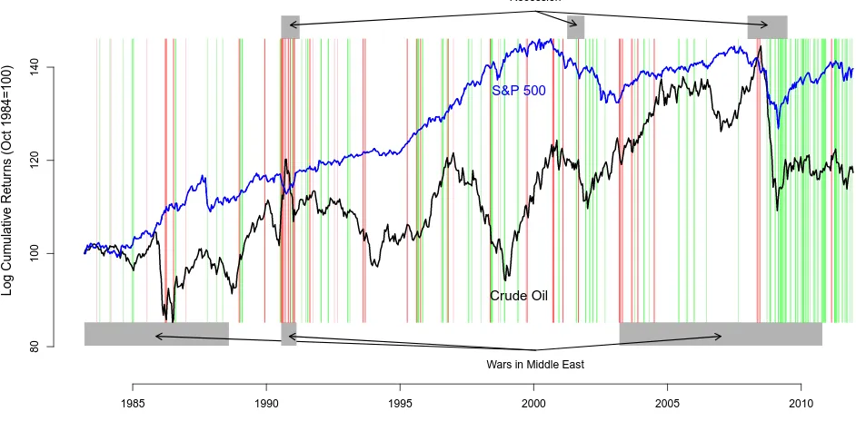
Figure 1.2: Performance of CL and S&P 500 in relation to Beta
Notes: βare shown on graph using vertical lines:
• All betas shown are statistically significant at 90% level
• Red:β≤ −1; light red:−1< β <0
Figure 1.2 shows the rate of return of Crude Oil futures and the S&P 500, as well as the bi-weekly betas during the period. Market betas included in this figure are all significant at the 10% significance level, i.e. their t values fall in the region of |t| > 1.833 1. There are 48 negative betas, and 91 positive betas, out of 750 bi-weekly observations. As the graph shows, besides the apparent shocks mentioned above, there are a few other points worth mentioning: 1. Beta changes dramatically from period to period, with a trend toward being positive over the recent years (more green indicating more positive betas). 2. Price rose steadily from 2003 to 2007 due to a combination of the effects of stagnant supply and high demand (Hamilton 2009), which is also supported by the graph where positive and negative betas alternate. It also spiked in mid-2008 (Declining inventory prior to mid-2008), which apparently panicked the market and dragged the economy deeper into recession. 3. The spike of the price of oil in mid-2008 was followed by a big plummet, after which the price began to follow the pace of economic development very closely, as indicated by the positive correlation between oil prices and the economy. Additionally, price return on Oil appears to be higher than the S&P 500 through 2009-2011 where β≥1 for most of the time.2
Results shown in Table (1.3) show that the realized excess return of crude oil varies consis-tently with beta even without error correction; but, we reject the null hypothesis that δ1 = 1 because of the attenuation bias. When the previous period’s estimated beta is used as the instrument, we tend to overestimate the risk , δ1 > 1, unlike the underestimation of risk in many previous studies. Using a more complex method of state space model, we fail to reject the conditional CAPM.
SIMEX runs with λchosen to go from 0 to 4 using an increment of 0.04, 100 iterations for each λ. We calculate the sample mean of 100 estimatedδ0sfor each chosenλand form a series of paired δ and λ. Using mean measurement error variance from short-window regression as the proxy of σ2, which is 0.81 about 62% of the total variation in estimated beta. We choose different fitting methods of the trend and extrapolate toλ=−1 to get theδcoefficients that are corrected for estimation errors. For fitting methods such as restricted cubic splines and natural splines, linear extrapolation is used given these are locally fitting methods. For polynomial fitting, we use polynomials of the corresponding orders in the extrapolation. In Figure 1.3, the black dots are simulation results for δ1, and each solid line correspond to one fitting method
1
10% critical value of student t with 8 degrees of freedom.
2
Roil = Rf+β(Rm−Rf)
≥ Rf+ 1(Rm−Rf)
= Rm
●●● ●●●● ●●●●● ●●●●●●●●●●●●●●●●● ●●●●●●●● ●●●●●●●●●●●●●●●●●●●●●●●●●●●●●●●●● ●●●●●●●●●●●●●●●●●●●●●●●●●●●●●●●
−1 0 1 2 3 4
0.0 0.5 1.0 1.5 Lambda Predicted V
alue of Slope Coef
.
Simulation Results
−1 0 1 2 3 4
0.0 0.5 1.0 1.5 Lambda ●●● ●●●● ●●●●● ●●●●●●●●●●●●●●●●● ●●●●●●●● ●●●●●●●●●●●●●●●●●●●●●●●●●●●●●●●●● ●●●●●●●●●●●●●●●●●●●●●●●●●●●●●●● 4 knots 5 knots 6 knots 7 knots 8 knots Natural Splines
−1 0 1 2 3 4
0.0 0.5 1.0 1.5 Lambda ●●● ●●●● ●●●●● ●●●●●●●● ●●●●●●●●●●●●●●●●● ●●●●●●●●●●●●●●●●●●●●●●●●●●●●●●●●● ●●●●●●●●●●●●●●●●●●●●●●●●●●●●●●● 5 knots 6 knots 7 knots 8 knots 9 knots Restricted Cubic Splines
−1 0 1 2 3 4
0.0 0.5 1.0 1.5 Lambda ●●● ●●●● ●●●●● ●●●●●●●● ●●●●●●●●●●●●●●●●● ●●●●●●●●●●●●●●●●●●●●●●●●●●●●●●●●● ●●●●●●●●●●●●●●●●●●●●●●●●●●●●●●● Order 3 Order 4 Order 5 Order 6 Order 7 Polynomial
Table 1.3: CAPM Results - Summary
F-Stat δ0×100 δ1
(p-value) (s.e×100) (s.e)
Standard OLS 38.47 0.08 0.44
(0.00) (0.23) (0.07)
IV Corrected 18.11 0.04 1.90
(0.00) (0.24) (0.45)
Kalman Filter 33.40 0.05 1.29
(0.00) (0.24) (0.22)
Notes: The tables shows the regression results of Equation 1.2:riτ =δ0+δ1( ˆβiτrM τ) +µiτ
1. Standard OLS:βs are estimated results of short-window regressions (Equation 1.1) without error correc-tion
2. IV Corrected:βs are corrected for using its lag as instrument
3. Kalman Filted:βs are filtered using state space model with Kalman filter
Table 1.4: Simulation Extrapolation Results using Different Fitting Methods
Natural Spline* Restricted Cubic Spline** Polynomial
df Intercept(×100) Slope Intercept(×100) Slope Intercept(×100) Slope (s.e.×100) (s.e.) (s.e.×100) (s.e.) (s.e. ×100) (s.e.)
3 0.10 0.62 0.09 0.60 0.10 0.72
(0.23) (0.09) (0.23) (0.09) (0.23) (0.11)
4 0.10 0.65 0.10 0.62 0.13 0.86
(0.23) (0.10) (0.23) (0.09) (0.23) (0.13)
5 0.10 0.67 0.10 0.65 0.17 1.04
(0.23) (0.10) (0.23) (0.10) (0.23) (0.15)
6 0.11 0.68 0.10 0.67 0.10 1.11
(0.23) (0.11) (0.23) (0.10) (0.23) (0.19)
7 0.11 0.69 0.10 0.67 0.19 0.62
(0.23) (0.11) (0.23) (0.11) (0.26) (0.28)
Notes:
1. * In Natural Spline, Knots = df +1
2. ** In Restricted Cubic Spline, Knots = df +2
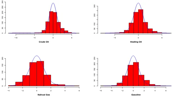
Table 1.5: Summary of Pricing Error (%)
Crude Oil Heating Oil Natural Gas Gasoline
Observations 750 864 567 706
Minimum -2.88 -2.84 -3.98 -2.94
25% -0.38 -0.38 -0.72 -0.42
Median 0.01 -0.01 -0.12 0.07
Mean 0.01 0.02 -0.14 0.03
75% 0.40 0.39 0.48 0.46
Maximum 3.48 3.10 4.07 3.22
Std Deviation 0.70 0.70 1.04 0.73
Skewness 0.08 0.12 -0.19 -0.08
Kurtosis 2.49 2.04 1.51 1.72
1.5
Testing other Energy Resources
In this section, we test CAPM using other energy commodities including unleaded gasoline, heating oil, and natural gas.3
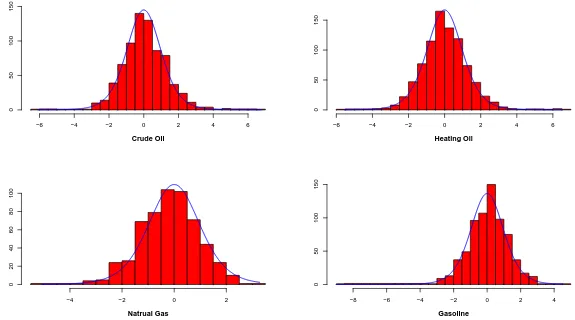
Pricing errors for each of these commodities are small and statistically insignificant as sug-gested by Table 1.5. Since alphas are estimated by using short-window regressions, the signifi-cance of each bi-weekly alpha will also show us how accurately CAPM can predict. Figure 1.4 includes the frequency distributions of the t-values for the estimated bi-weekly alphas for each commodity, and the blue line is the student t distribution with 8 degrees of freedom as a ref-erence4. If the red histogram bars can fill in the area under the blue line, it indicates that the t-values of bi-weekly alpha follows the t-distribute with zero mean. The figure provides us with evidence that the realized distribution of the pricing error fit the student t distribution well for all commodities, and no commodity has more high/low return than is predicted by the CAPM. 5
3Together with Crude Oil, these four commodities are the energy commodity futures closely monitored by
the Commodity Futures Trading Commission (CFTC).
4Bi-weekly alphas are estimated using 10 observations in each calendar week. 5
Crude Oil
Frequenc
y
−6 −4 −2 0 2 4 6
0
50
100
150
Heating Oil
−6 −4 −2 0 2 4 6
0
50
100
150
Natrual Gas
−4 −2 0 2
0
20
40
60
80
100
Gasoline
−8 −6 −4 −2 0 2 4
0
50
100
150
Figure 1.4: T-values of Estimated Pricing Error
Notes:
Table 1.6: Summary of Market Betas
Crude Oil Heating Oil Natural Gas Gasoline
Observations 750 864 567 706
Minimum -8.11 -8.22 -4.55 -6.97
25% -0.47 -0.47 -0.66 -0.49
Median 0.03 0.07 0.02 0.09
Mean 0.01 0.01 0.08 0.05
75% 0.60 0.53 0.67 0.62
Maximum 6.79 6.16 12.32 7.29
Std Deviation 1.14 1.10 1.58 1.14
Skewness -0.59 -0.78 1.55 -0.06
Kurtosis 7.59 9.52 10.20 5.58
Crude Oil
Frequenc
y
−10 −5 0 5
0
50
100
150
200
250
300
Heating Oil
−5 0 5
0
50
100
200
300
Natrual Gas
−4 −2 0 2 4 6
0
50
100
150
200
Gasoline
−6 −4 −2 0 2 4 6
0
50
100
150
200
250
Figure 1.5: T-values of Estimated Market Betas
Notes:
1980 1990 2000 2010
−50
0
50
100
150
Log Cum
ulativ
e Retur
ns (J
an 2000 = 100)
Recession
Wars in Middle East
S&P 500
Crude Oil
Heating Oil
Natural Gas
Gasoline
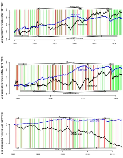
Natural Gas has a different risk profile from crude oil, despite the fact that it is also an exhaustible natural resource like crude oil. Locally supplied natural gas isolates it from disrup-tions in supply caused by conflicts in the Middle East, but price spikes in crude oil can still lead to higher natural gas prices due to substitution effects, as we can see in the recent price spike in mid-2008. Recent technological advances have enabled us to extract natural gas from shale rock, which greatly affected production. The recent decrease in gas prices from 2007-2011 is likely caused by a combination of recession (demand) and technology (supply) as shown in Figure 1.7, while petroleum products were likely driven mainly by demand fluctuations. Since natural gas is used to heat more than half of the homes in America, short-term demand for natural gas can also be affected greatly by cold temperatures, making both its prices and its market beta fluctuate. Big short-term demand shocks induced by weather lead to a high occurrence of positive betas, and the market beta for natural gas is positive on average.
1985 1990 1995 2000 2005 2010 80 100 120 140 160 Log Cum ulativ e Retur
ns (Oct 1984=100)
Recession
Wars in Middle East
Gasoline S&P 500
1980 1990 2000 2010
80 100 120 140 160 Log Cum ulativ e Retur ns (No
v 1978 =100)
Recession
Wars in Middle East
Heating Oil S&P 500
1990 1995 2000 2005 2010
0 50 100 Log Cum ulativ e Retur
ns (Apr 1990=100)
Recession
Wars in Middle East
Natural Gas
S&P 500
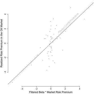
−4 −2 0 2 4
−4
−2
0
2
4
CAPM Prediction
Realiz
ed Risk Premium
Perf
ect CAPM Predictions Crude Oil
Heating Oil Natural Gas Gasoline
−4 −2 0 2 4
−4
−2
0
2
4
Error−Corrected CAPM Prediction
Realiz
ed Risk Premium
Table 1.7: CAPM Results - Summary
Standard IV Corrected Filtered
Commodity δ0×100 δ1 δ0×100 δ1 δ0×100 δ1
(s.e×100) (s.e) (s.e×100) (s.e) (s.e×100) (s.e)
CAPM Predictions: δ0 = 0 and δ1 = 1
Crude Oil 0.08 0.44 0.04 1.90 0.05 1.29
(0.23) (0.07) (0.24) (0.45) (0.24) (0.22)
Heating Oil 0.11 0.33 0.07 2.04 0.07 1.12
(0.22) (0.07) (0.22) (0.72) (0.22) (0.21)
Natural Gas -1.08 0.26 -1.05 2.44 -1.04 0.91
(0.39) (0.09) (0.39) (1.59) (0.39) (1.51)
Gasoline 0.30 0.42 0.30 2.84 0.27 1.23
(0.25) (0.08) (0.25) (0.66) (0.25) (0.23)
Notes: The tables shows the regression results of Equation 1.2:riτ =δ0+δ1( ˆβiτrM τ) +µiτ
1. Standard:βs are estimated results of short-window regressions (Equation 1.1) without error correction 2. IV Corrected:βs are corrected for using its lag as instrument
Table 1.8: SIMEX results for Energy Commodities
Natural Spline* Restricted Cubic Spline** Polynomial***
Commodity Intercept(×100) Slope Intercept(×100) Slope Intercept(×100) Slope (s.e.×100) (s.e.) (s.e.×100) (s.e.) (s.e.×100) (s.e.)
Crude Oil 0.10 0.65 0.10 0.62 0.11 0.85
(0.23) (0.10) (0.23) (0.09) (0.24) (0.13)
Heating Oil 0.13 0.51 0.12 0.49 0.14 0.71
(0.22) (0.10) (0.22) (0.10) (0.22) (0.14)
Natural Gas -1.12 0.42 -1.11 0.40 -1.17 0.65
(0.39) (0.12) (0.39) (0.12) (0.39) (0.17)
Gasoline 0.29 0.66 0.29 0.63 0.29 0.93
(0.25) (0.12) (0.25) (0.11) (0.25) (0.17)
Notes:
1. * Natural Spline of 5 knots
1.6
Conclusion
Using high frequency energy futures data, we estimate a series of bi-weekly betas using CAPM and document a strong relationship between energy futures prices and the aggregate economy. Unlike previous studies, where betas for stocks are mostly close to 1 and zero for commodities, our model shows great variability in the betas for a single commodity over time that vary from strongly positive to strongly negative, and significant differences in betas across different com-modities, reflecting fundamental differences in the nature of supply and demand and connection to the macro economy.
The market beta displays a significant amount of price variation in the energy market and we fail to reject conditional CAPM, correcting for measurement error. Realized risk premium, however, appears to increase more rapidly than one-to-one with CAPM-based risk, after mea-surement error is corrected with IV. An area for further investigation is to explain why there appears to be too much covariance risk pricing, rather than too little as previous studies indi-cate.
Chapter 2
Discounting Investments that Save
Energy Resources
2.1
Introduction
Relative to traditional technologies, investments in renewable energy and energy-conserving technologies involve higher up-front costs in exchange for a lower stream of future operating costs. The discount rate for future expected operating costs is therefore central to the investment decision.
Recent research has emphasized the importance of uncertainty about the discount rate, especially when investments are long-lived. Because present values are convex in the discount rate, uncertainty about the rate combined with Jensen’s inequality implies that optimal in-vestment decisions are governed by a relatively low certainty-equivalent rate that declines with the investment’s duration (Weitzman 1998, Weitzman 2001, Newell and Pizer 2003). This past research has emphasized discounting public investments to curb global warming, given the espe-cially long time horizon and vigorous debate (and thus uncertainty) about which discount rate should be used (Stern 2006, Tol 2006, Nordhaus 2007, Dasgupta and Maskin 2005, Weitzman 2007 etc). But uncertainty about future discount rates could be important to many kinds of investments, public and private. And while more tangible investments in renewable energy or energy-conserving technologies surely have shorter durations than broader public policies to curb global warming, the horizons are long enough for uncertainty to matter.
has not been systematically measured accounting for stochastic variations in interest rates, risk premiums and the operating costs themselves. Our central contention is that careful account of these uncertainties substantially influences optimal investment decisions.
Modeling discount rate uncertainty requires systematic decomposition of the size and stochas-tic evolution of its components. A natural starting point for the analysis follows Newell and Pizer (2003), who estimated long-run discount rate uncertainty using time-series analysis of historic real interest rates. In addition to stochastic variations in interest rates, in this pa-per we simultaneously account for (a) uncertainty about energy prices; (b) uncertainty about overall-market risk premiums; and (c) uncertain and time-varying risk premia of energy savings. Risk premiums for energy-related investments are particularly important given connections between oil prices and the macroeconomy (Hamilton 1983, Barsky and Kilian 2004, Kilian 2009). Historically, price spikes in oil and other energy resources have been associated with supply shocks or with speculative demand driven by fear of future supply shocks. Such shocks are classic examples of negative aggregate supply shocks for the macroeconomy, and should thus have negative risk premiums. But not all oil prices shocks are alike (Kilian 2009). More recent spikes in oil prices can be connected to positive aggregate demand shocks, particularly growth in Asia, which would logically have positive risk premiums (Hamilton and Wu 2011, Kilian 2009). Thus, events that drive energy price variations suggest that underlying risk premiums may be large, positive or negative, and time varying, giving rise to considerable uncertainty about future risk-adjusted discount rates of energy-conserving investments. In quantifying all of these uncertainties simultaneously, we essentially attempt to rigorously quantify the value of so-called “energy security.”
Following the Capital Asset Pricing Model (CAPM), the risk premium equals an overall-market risk premium multiplied by the investment-specific beta. Thebeta measures the covari-ance between returns of a specific investment and returns of the overall market. Whereas the overall-market risk premium is always positive, its size is also time varying, particularly with macroeconomic business cycles. Beta, per the discussion above, can also be time-varying, but may be positive or negative. For example, an unexpected discovery of a large new oil deposit would cause oil prices to decline while simultaneously providing good news for the aggregate economy and stock returns. Such an event would be embodied by a negative beta and risk pre-mium. Conversely, larger-than-expected growth in emerging markets may drive up aggregate demand, increasing both overall-market returns and oil prices, giving rise to a positive beta
and risk premium. The discount rate is comprised of the investment-specific risk premium plus a risk-free (or zero-beta) interest rate. The risk-free rate can also vary over time, and will be uncertain over long horizons, as modeled by Newell and Pizer.
uncertainty about those rates. Given the stochastic nature of the discount rate, we derive constant-equivalent discount rates for different time horizons for comparisons and discussions. The constant-equivalent discount rate is defined in this paper as the constant discount rate that will produce the same expected present value of the future net benefit assuming energy prices and consumption stays at current level. These constant-equivalent rates may serve as useful guides for energy-related investment decisions.
We begin by modeling a simple stylized model of a consumer facing a choice between two cars with identical features except fuel efficiency. This simplified example helps set up the connection between the expected present value of the future net benefits and the constant-equivalent discount rate. In the absence of any private value attached to the social benefits of fuel economy on the environment, the consumer chooses between the higher up-front cost of a fuel-efficient car and the higher stream of energy cost of the standard car. The present value of the total savings on future energy spending is central to this choice, which depends on both energy prices and discount rates. For this simplified example, we assume all other attributes of the car, like performance, utility, and aesthetic appeal, are held constant.
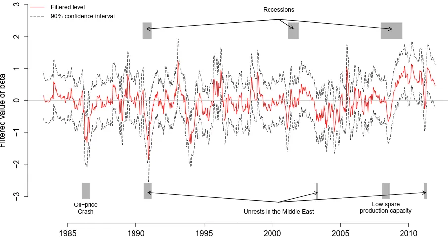
We first estimate series of bi-weekly energy-specific betas estimated using a time-varying CAPM. Because estimated betas contain large sample errors, we then use a state-space model to filter the error and estimate the stochastic evolution of the underlying truebeta. We model the energy prices, the market risk-premium and the risk-free rate with a vector autoregressive model (VAR) to allow the variables to covary with each other and account for heteroskedasticity using a generalized autoregressive conditional heteroskedasticity (GARCH) model. After estimating these models using past data of energy prices, we forecast future values and uncertainties using Monte Carlo simulation. We use elasticities from the existing literature to account for adjustments in vehicle miles traveled and associated surplus changes in response to projected energy prices. To estimate the expected present value of the net savings on future energy costs, we integrate the distribution of risk-adjusted savings by simulating the estimated model 1,000 times, calculating the realized present value of savings in each iteration, and taking the average. We find that the conditional CAPM has strong predictive power over the risk premia in the oil market and fail to reject the model when estimation errors in beta are corrected for using the Kalman Filter. By allowing beta to vary at relatively high frequency, the time path of filtered beta captures many of the historical shocks in the oil market. Over the time period from 1983-2011, crude oil has had an average -0.37% annual risk premium, assuming an overall market risk premium of 5%, but it varied significantly from positive to negative over time in response to the market changes (such as recessions and booms), as well as shifts in oil supply (such as those caused by unrest in the Middle East).
assume betas follow a stationary autoregressive (AR) process. We find that the greater the uncertainty, the higher the present value of total energy saving, and thus the lower the certainty-equivalent discount rate. Few investments actually save oil, but rather gasoline or electricity or some composite of energy resources, although prices of substitute energy resources tend to be correlated. Further, consumption behavior would presumably change in response to prices. People will drive less if gasoline prices rise. Taking these into account for a vehicle, our estimate of an implicit discount rate ranges from 18% in the most conservative model setup, to -20% in the most uncertain for the 5-year time horizon.
When we expand the calculations to cover the lifetimes of other, longer-lived energy-related investments, we find that the more distant into the future, the lower the discount rate for each model specification due to the rising uncertainty with time. With the most conservative method, where beta follows an AR(1) and other variables follow VAR(1) with no trend, the annualized discount rate falls from 18% in 5 years to 6% in 25 years, 3.7% in 50 years, and 2% in 100 years. Whereas adding a linear trend to the VAR model and keeping other specifications unchanged, the annualized discount rate becomes 16% in 5 years, 3% in 25 years to -3.62% in 100 years. To further illustrate how high levels of uncertainty may affect the constant-equivalent discount rate, we include models with quadratic time trend which have the higher level of uncertainty; and its predicted discount rates are much lower for all different lifetimes of projects -14%, -19% and -39% respectively. The qualitative results fit the declining pattern both Weitzman (1998) and Newell and Pizer (2003) found, where Newell and Pizer conclude that certainty-equivalent discount rate have declined from 4% to 2% after 100 years, using interest rate as the single component in the discount rate and ignoring the risk component.
2.2
A Simple Numerical Example
The present value of the total energy savings over a N-period horizon is equal to
S =P1Qs1exp(−δ1) +P2Qs2exp(−δ1−δ2) +...+PNQsNexp − N X t=1 δt ! . (2.1)
wherePt is the price of energy,Qst is the amount of fuel that consumer can save by driving the hybrid rather than the standard, andδt is the risk adjusted discount rate, defined as
δt=rt+γt, (2.2)
withrtdenoting risk-free interest rate and γt the risk premium.
An essential consideration is the fact that prices Pt and future discount rates δt are not
known to the consumer in advance. Further, the consumer’s expectations aboutPtand δt may well be correlated. The law of one price rules that the price of an asset equals to its expected discounted payoffs.
pt=Et[∆t+1xt+1]
where ∆t+1is the intertemporal marginal rate of substitution, or the stochastic discount factor, and xt+1 is the asset’s payoff.
In the consumption-based asset pricing models, the stochastic discount factor is often defined as
∆t+1=ρ
u0(ct+1)
u0(c
t)
whereρis the subjective rate of time preference, andu0(c) is the marginal utility of consumption. To further illustrate how prices and discount rate may be correlated, from the first equation above we can get:
1 =Et
xt+1
pt
∆t+1
=Et[(Rt+1)∆t+1]
=Et(Rt+1)Et(∆t+1) +Covt(Rt+1,∆t+1) (2.3)
whereRt+1 is the gross return of the asset. Equation (2.3) can be rewritten as:
Et(Rt+1) =
1−Covt(Rt+1,∆t+1)
Et(∆t+1)
(2.4)
con-sumption substitution, i.e. the stochastic discount factor, and thus earn a positive risk premium and have a higher expected return. Such an asset typically has a low return when investors’ consumption levels are low (marginal utility is high) and the asset is perceived as risky because it does not provide wealth when it is needed most. Therefore, investors will demand higher premia to compensate for the risk they bear holding such assets.
Our general form of the net present value of total energy saving (Equation 2.1) can fully embody such correlation and provide us with better understanding of how savings would change given uncertain prices, consumption levels, discount rates and their potential correlations. The next step is to model how these variables have evolved historically using time series econometric models. We will then forecast from the estimated models to quantify trends and uncertainty in
Ptand δt.
2.3
Estimating Risk Premium using the Capital Asset Pricing
Model
The Capital Asset Pricing Model (CAPM) ties the scholastic discount factor to the return on the wealth/market portfolio and is most often expressed in its beta-representation. It states that the risk premium equals an overall-market risk premium multiplied by the investment-specificbeta, which measures the covariance between the returns of a specific investment and returns of the overall market. Similar to the covariance between prices and the marginal rate of consumption substitution in Equation (2.4),beta is also a good measure of risk and an important component of the risk premium. For example, an asset that co-varies negatively with the overall market would become a good hedge against bad economic times protecting consumers like an insurance. Thus, such asset would be perceived as less risky and warrant a smaller risk premium.
Following the CAPM, we can rewrite Equation (2.2) as:
δt=rt+βtγtM, (2.5)
whereβt is the asset-specific beta andγtM is the market risk premium. The overall-market risk
premium is always positive and its size generally varies with time, particularly with macroe-conomic factors such as unemployment and growth. Markets become riskier in bad emacroe-conomic times such as recessions, therefore investors demand higher risk premia to compensate for the extra risk they bear. And the poorer the state of the economy is, the higher is the risk premium demanded by the investors.1
The asset-specificbeta can also vary over time, but can be either positive or negative, espe-cially for energy-saving investments. For example, an unexpected shift in supply, like discovery
1
of a large new oil deposit, would cause oil prices to decline, while simultaneously providing good news for the aggregate economy and stock returns. Such an event would be embodied by a negative beta and risk premium. Conversely, the repeatedly faster-than-expected growth in Asia may drive up aggregate demand, increasing both overall-market returns and oil prices, giving rise to a positive beta and risk premium. Similarly in the recent work by Kilian (2009), he attributes the recent rise in oil price mostly to the positive demand shock. The relative frequen-cies of such events may change over time, sometimes quite frequently, causing large variations inbeta that cannot be captured by the static CAPM many previous studies have adopted.2
To allow betas to change with high frequency, we follow Lewellen and Nagel (2006) and directly estimate betas and risk premia unconditionally through short-window (bi-weekly) re-gressions to generate an estimate forbeta in each two-week period t:
γi=α+βγiM+νi (2.6)
i= 1,· · ·,10
where γi and γiM are asset risk premia and market risk premium on the ith day within each time period, respectively.
Short-window regressions give unbiased estimates of the average beta within each window. A short window therefore allows for relatively unconstrained changes in beta over time. The tradeoff is that the small sample size within each window results in large estimation error. Below, we will consider state-space methods for filtering this error to uncover the underlying process for the true beta.
The state space model is a flexible form that can be formulated to model dynamic time series with measurement errors. The state space representation of short-window betas can be written as:
ˆ
βt=βt+t (2.7)
βt=φ0+φ1βt−1+υt (2.8)
wheret∼N(0, V) and υt∼N(0, W).
Equation (2.7) states that the ˆβtestimated using the short window regressions is composed of the truebeta,βt, and the estimation error,t. Despite the fact thatbeta may change significantly
over time, the nature of uncertainty could likely be similar enough from week to week and there is some level of persistence. The transition equation (2.8) aims to capture the persistence of
beta over time and assumes that the truebeta follows an autoregressive process.
In the presence of heteroskedastic disturbances, the statistical inferences on estimates from
2
the basic space state model will be inefficient. In this paper, we adopt the method derived in Harvey, Ruiz and Sentana (1992) and Kim and Nelson (1999), and combine the state space model with the Generalized Autoregressive Conditional Heteroskedasticity (GARCH) process to model the disturbances. That is, if the distributions of both t and υt depend on the past
information up tot−1, they can be modeled by the GARCH process.
In order to do this, we define the conditional distributions of disturbances as t|ψt−1 ∼
N(0, h1,t) and υt|ψt−1 ∼ N(0, h2,t), where ψt−1 refers to the information set up to t−1. h1,t
and h2,t follow this GARCH(1,1) process:
h1,t=a0+a1t2−1+a2h1,t−1
h2,t=b0+b1υt2−1+b2h2,t−1 (2.9)
Rewriting the model into the canonical state space form, we have:
ˆ
βt= h
1 1 0 i βt t υt
( ˆβt= H βt∗)
βt t υt = φ0 0 0 +
φ1 0 0
0 0 0
0 0 0
βt−1
t−1
υt−1 + 0 1 1 0 0 1 " t υt #
(βt∗ = µ∗ + F βt∗−1 + G υt∗)
where
E(υ∗tυt∗0|ψt−1) =
"
h1,t 0
0 h2,t
#
=Rt
Prediction equations:
βt∗|t−1 =E(β∗t|ψt−1)
=µ∗+F βt∗−1|t−1
Pt∗|t−1 =Eh(βt∗−βt∗|t−1)(βt∗−βt∗|t−1)0i =F Pt∗−1|t−1F0+GRtG0
ηt|t−1 = ˆβt−E( ˆβt|ψt−1) = ˆβt−Hβt∗|t−1
ft|t−1 =E(ηt2|t−1)
=HPt∗|t−1H0 (2.10)
Updating equations:
β∗t|t=E(β∗t|ψt)
=βt∗|t−1+Pt∗|t−1H0ft−|t1−1ηt|t−1
Pt∗|t=Eh(βt∗−βt∗|t)(β∗t −βt∗|t)0i
=Pt∗|t−1−Pt∗|t−1H0ft−|t1−1ηt|t−1 (2.11)
In Equation (2.9) 2t−1 and υ2t−1 are unobserved. To account for this unobservability, we adopt the same remedy as in Harvey, Ruiz and Sentana (1992), and instead estimate with their conditional expectations:
h1,t=a0+a1E(2t−1|ψt−1) +a2h1,t−1
h2,t=b0+b1E(υ2t−1|ψt−1) +b2h2,t−1 (2.12)
Also,
E(2t−1|ψt−1) =E(t−1|ψt−1)2+E
(t−1−E(t−1|ψt−1))2
E(υt2−1|ψt−1) =E(υt−1|ψt−1)2+E
(υt−1−E(υt−1|ψt−1))2
(2.13)
whereE(t−1|ψt−1) andE(υt−1|ψt−1) are the last 2 elements ofβ∗t−1|t−1; and
E
(t−1−E(t−1|ψt−1))2
and E
(υt−1−E(υt−1|ψt−1))2
are the last two diagonal elements of Pt∗−1|t−1.
variance, ft|t−1, which we obtained using a Kalman filter. The log likelihood function can be written as:
ln(L) =−0.5
T
X
t=1
lnh2πft−|t1−1i−0.5
T
X
t=1
ηt0|t−1ft−|t1−1ηt|t−1 (2.14)
2.4
Vector Autoregressive Models
The risk-free return, market return and commodity prices are modeled using Vector Autore-gressive Process of order p (VAR(p)). To increase the predictive power, we also include in the VAR model the Cyclically Adjusted Price Earnings Ratio (CAPE), whose explanatory power over the long run market return was successfully demonstrated in the book, Irrational Exuber-ance, by Shiller (2005). To ensure the non-negativity of prices and the CAPE, both variables are modeled in their natural logarithm form, resulting in:
yt=A0+A1yt−1+...+Apyt−p+ut, (2.15)
where
yt=
ln(Pt)
rtM rt ln(capet)
and ut=
u1,t u2,t u3,t u4,t
The conditional distributions of disturbances are defined asui,t|ψt−1 ∼N(0, gi,t)∀i= 1· · ·4; and gi,t follows a GARCH(1,1) process.
gi,t =ci,0+ci,1u2i,t−1+ci,2gi,t−1, i= 1,2,3,4
To compare how model specification would affect the savings and discount rates, we also included cases of VAR(p) with a linear trend, quadratic trend, and price trend interaction. There is a prominent downward trend in risk-free rate of return, predictions of risk-free return will be dominated by the extrapolation of time trend and lead to spurious results; therefore risk-free returns are modeled without time trend for all different model specifications.
2.5
Fuel consumption estimation
In Equation (2.1), the amount of fuel saved every period depends on the total consumption and relative fuel efficiency. According to the US department of Energy, the 2012 Honda Civic has an average EPA MPG of 32 for the standard version, and 44 MPG for the hybrid version.3 This means that a consumer saves about 25% of the total gas consumption by driving a hybrid rather than standard Civic.
To simplify the model, we estimate the energy consumption using the short-run price elas-ticities of demand and prices forecasts.
Qst = 0.25Qt
whereQt is the gasoline consumption when driving a standard Civic, at time t. The price elasticity of demand is defined as:
e= lnQt+1−lnQt
lnPt+1−lnPt
(2.16)
Using the two equations above, we are able to see that consumption savings change in response to price change and chosen elasticity, given by:
Qst+1= 0.25exp{[lnQt+e(lnPt+1−lnPt)]} (2.17)
2.6
Path-wise Simulations for
βt
,
rt
,
r
Mt,
Pt
and
Q
stThe prediction equations for each of the variables used to create this model are:
βT+t=φ0+φ1βT+t−1+υT+t
yT+t=A0+A1yT+t−1+...+ApyT+t−p+uT+t
QsT+t= 0.25exp{[lnQT+t−1+e(lnPT+t−lnPT+t−1)]}
h2,T+t=b0+b1υ2T+t−1+b2h2,T+t−1
gi,T+t=ci,0+ci,1u2i,T+t−1+ci,2gi,T+t−1, i= 1,2,3,4 (2.18)
whereT refers to the end period of the observed data. Due to the serial dependence of the time series data, we calculate the future values using their lags and instantaneous random shocks. This proceeds as follows:
3
1. At timeT, randomly draw 1,000 sets ofβT,υT anduT from their estimated distributions.
To simplify calculations, we normalizeln(QT) to 1;
2. At time T+t, calculate the variances of disturbances, h2,T+t and gi,T+t, using past
real-izations of the error terms and lag variances. Draw instantaneous disturbances υT+t and ui,T using the updated distributions;
3. CalculateβT+t,yT+tandQsT+tfollowing the equations listed above using their lag values
and the random disturbances drawn in step 2.
4. Repeat step 2 and 3 ∀t = 1,· · · , N. And the distributions for time horizons, N, are se-lected according to typical lifetimes of prominent energy-related investments, like vehicles, household appliances, photo-voltaic solar panels, and windmills.
2.7
Data and Estimation Results
We choose crude oil for the study because gasoline prices are closely related to the price of crude oil, and more importantly, crude oil prices have a bigger influence over energy policies, given its market share (37% of the U.S. energy consumption4), the turbulent market conditions and its well-documented connections with the overall economy (Hamilton 1983, Barsky and Kilian 2004, Kilian 2009).
The daily crude oil spot prices are obtained from the Commodity Research Bureau (CRB). The excess returns are defined as:
γt=ln(Pt)−ln(Pt−1)−rf t
S&P 500 indices are used as the proxy for the market portfolio, the indices, dividends, and earnings data are obtained from the Standard and Poor’s online database.5 Its price returns, used in the vector autogressive model in Section 2.4, is defined as:
rMt =ln(SPt+Dividendt)−ln(SPt−1).
where daily dividend is calculated from the quarterly ones, and the excess market return is:
γtM =rtM −rf t
We use 3-month Treasury bill as our risk-free asset, and follow the standard yield calculation on the Treasury bill and the return is:
rf t=
h
1
1−DT B3t·(91/360)
i(days/91)
−1
where DT B3t is the daily quotation in the secondary market on the most recently auctioned
Treasury Bills for 3-month maturity. The daily rate is from FRED.®6 The rate will be used 4
Source:http://www.eia.gov/totalenergy/data/annual/pdf /sec19.pdf, percentage is calculated using share
of Btu.
5
Source:http://www.standardandpoors.com/indices/sp−500/en/us/?indexId=spusa−500−usduf− −p−us−l− −.
6