An analysis of steady state void fraction distribution and steam void response to sinusoidal power modulation in a boiling water coolant channel.

(1)

Scholarship at UWindsor

Electronic Theses and Dissertations Theses, Dissertations, and Major Papers

1-1-1967

An analysis of steady state void fraction distribution and steam

void response to sinusoidal power modulation in a boiling water

coolant channel.

Afamefuna E.A. Egbuniwe University of Windsor

Follow this and additional works at: https://scholar.uwindsor.ca/etd

Recommended Citation Recommended Citation

Egbuniwe, Afamefuna E.A., "An analysis of steady state void fraction distribution and steam void response to sinusoidal power modulation in a boiling water coolant channel." (1967). Electronic Theses and

Dissertations. 6472.

https://scholar.uwindsor.ca/etd/6472

(2)

AN ANALYSIS OF STEADY STATE VOID FRACTION DISTRIBUTION AND STEAM VOID RESPONSE TO SINUSOIDAL POWER

MODULATION IN A ROILING WATER COOLANT CHANNEL

A Thesis

Submitted to the Facultylof Graduate Studies through the

Department of Chemical Engineering in Partial Fulfilment

of the Requirements for the Degree of

Master of Applied Science at

University of Windsor

by

Afamefuna E.A.Eghuniwe

Windsor,Ontario

(3)

IN F O R M A T IO N T O U S E R S

T h e quality of this reproduction is d ep e n d e n t upon th e quality of th e copy

subm itted. B roken or indistinct print, colored or poor quality illustrations and

photographs, print bleed-through, sub standard m argins, and im proper

alig n m en t can a d versely a ffect reproduction.

In the unlikely e v e n t that the auth o r did not send a co m p lete m anuscript

and th e re are missing pages, th e s e will be noted. Also, if unauthorized

copyright m aterial had to be rem o ved , a note will indicate th e deletion.

UMI

U M I M icroform E C 5 2 6 5 3

C opyright 2 0 0 8 by P ro Q u e s t LLC.

unauthorized copying u n d er Title 17, United S ta te s C ode.

P ro Q u e s t LLC 7 8 9 E. E ise n h o w e r P arkw ay

(4)

4 6 / f 6 7 3 7

APPROVED BY;

(5)

In this theoretical analysis,various models and correlations were

-tested for their ability to predict correctly the steady state Gross-

sectional average void fractions in a boiling water channel. A modified

Bowring’s model is proposed and then employed to predict the steam weight

fraction distribution in the subcooled boiling region. This modified model

is used also in the theoretical prediction of steam void, response to small

power perturbation in a boiling water channel.

Bowring’s model (l),was employed to predict the inception of the

subcooled boiling region. In this subcooled boiling region,a parameter

e was introduced to relate the heating component to the evaporative

component of the total heat flux. The parameter e was assumed to vary

linearly throughout the subcooled boiling region. In the bulk boiling

region, ;e equals zero, and the steam weight fraction distribution is calcu

lated from a thermal energy balance.

Various theoretical models and correlations were tested agaist available

experimental data {17,29,36) for their ability to predict accurately the

steam void fraction for both the subcooled boiling region and the bulk

boiling region. Satisfactory agreement was obtained with the majority of

the models over a wide range of channel geometries, heat fluxes, pressure

and inlet flow rates. Neal’s model (7) was found to give the best overall

ag r e e m e n t . The range of operating conditions considered were ;

Pressure ILO-IOOO psia

(6)

Flow Area rectangular,annular,

, and circular

Inlet Liquid Velocity above 2 ft/sec.

Subcooling 1.1°F to 21.6°F

Heat Flux 22,800-157,OOOBtu/hr-ft^

In the unsteady state analysis, the equations of change were written

in the one-dimensional macroscopic form, differenced in the height variable

and solved employing a stagewise complex integration procedure. Improved

agreement with experimental data (36) was obtained employing the modified

(7)

The author wishes to express sincere thanks to Dr. C.C. St; Pierre for

his help and guidance, to Atomic Energy of Canada, Chalk River, Ontario,

for the use of the CDC-G20 computer, and to Mrs. S. Ouellette of the

Electrical Engineering Department for the use of a typewriter^

The financial assistance from the National Research Council and

(8)

■ ■ CONTENTS.

ABSTRACT 111

ACKNOWLEDGEMENTS v '

LIST OF FIGURES vili

CHAPTER I INTRODUCTION 1

CHAPTER II LITERATURE SURVEY

A . Cross-sectional Average Void Fraction A

1. Bulk Boiling Region

2. Subcooled Boiling Region

B. Theoretical Models for the Dynamics of 7

Coolant Channels

C. Power to Void Transfer Function Measurement 9

/ CHAPTER III PRESENT ANALYSIS

A. Bowring’s Model 12

B. Proposed Modification of Bowring’s Model 13

C. Unsteady State Analysis - 15

CHAPTER IV MACROSCOPIC EQUATIONS OF CHANGE FOR A Tim-PHASE

FLOWING SYSTEM

A . Basic Equations 17

1. Macroscopic Mass Balance

2. Macroscopic Momentum Balance

3. Macroscopic Energy Balance

A . Channel Wall Energy Balance

B. Dimensionless form of Equations of Change 19

C. Steady State Equations 21

1. Non-boiling Region

A . Boiling Region Transitions

D. Unsteady State Equations of Change 28

CHAPTER V DISCUSSION

(9)

NOMENCLATURE

REFERENCES

APPENDIX III

VITA AUCTORIS

Vll

55 59

APPENDIX I 65

APPENDIX II 56

70

APPENDIX IV

(10)

LIST OF FIGURES

FIGURES

1 Void Fraction Prediction Using the Modified Powring's 42

Model and Powring's Model with Experimental Data (Ref. 17).

2 Void Fraction Prediction Using the Modified Rowring's 43

Model and Bowring's Model with Experimental Data (Ref. 17).

3 Comnarison of Christensen's Experimental Data (Ref. 2D) 44 with Values Predicted by Modified Bowring's Model Run 2 •

4 Comparison of Christensen's Experimental Data (Ref. 29) 45 with Values Predicted bv Modified Bowring's Model Run IjO.

5 Comparison of Christensen's Experimental Data (Ref. 29) 46 with Values D^pdicted by Modified Rowring's Model Run

6 Comparison of Christensen's Experimental Data (Ref. 29) 47 with Values Predicted by Modified Bowring's Model Run 16.

7 Comparison of St. Pierre's Experimental Data (Ref.36) with • 48 Values Predicted by Modified Bowring's Model and constant e

Run 12.

8 Comparison of St. Pierre's Experimental Data (Ref.36) with Lg Values Predicted by Modified Bowring's Model and constant

Run _6.

9 Comparison of St. Pierre's Experimental Data (Ref.36) with' 50 Values.Predicted by Modified Bowring's Model and constant je

Run §_•

10 Comparison of St. Pierre's Experimental Data (Ref.36) with 51 Values Predicted by Modified Bowring's Model and constant e

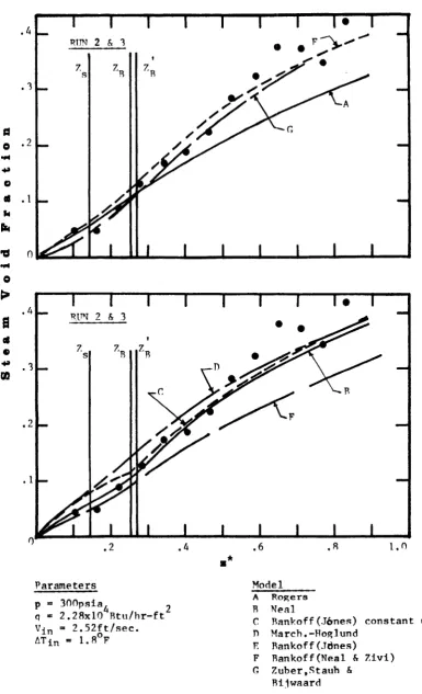
Run 2&3.

11 Comparison of Christensen's Experimental Data (Ref.29

)

with 52 Values Predicted by an assumed Linear Variation of Slip Ratio

with axial distance.in the Subcooled Boiling Region, Run 10.

12 Comparison of Christensen's Experimental Data (Ref.29

)

with 53 Values Predicted by an assumed Linear Variation of Slip Ratio

with axial distance in the Subcooled Boiling Region, Run 12.

13 Comparison of Power-to-void transfer Data(Ref.36) with Values 5^ Predicted by the Modified Bowring's Model and e = 1.3.

(11)

In a boiling water reactor, there is an inherent interraction of

reactor power output with the volume void fraction present in the

core. Consequently, a knowledge of the vapour volume distribution along

the channel axial length is of importance for reactor design since

this interraction can result in boiling water reactor instabilities.

Instabilities can arise from reactivity feedback, causing divergent

power oscillations, or from hydrodynamic instability which may occur

in natural circulation boiling systems at constant power.

The steady state behaviour and the dynamic response of a reactor

are strongly dependent on the vapour volume distribution present in

the core. Theoretical predictions of the vapour volume distributions

in a channel are often complicated, due to the presence of three

boiling regions: a non-boêiing region, a subcooled boiling or non-equi

librium region, and a bulk boiling region. In addition, the boundaries

between these regions must be considered.

Several attempts have been made by different authors to formulate

theoretical models or semi-empirical correlations to predict vapour

volume distribution in a boiling water channel. At present there is no

m o d e l o r c o r r e l a t i o n which can be used f o r all of the possible operating

conditions in present day reactors. In general, the semi-empirical

correlations employ dimensionless groups which the authors believe to

(12)

predictions employing these correlations cannot be extrapolated with any

degree of confidence beyond the experimental data used to obtain the

correlations.

Authors in deriving the theoretical models have employed many

assumptions because of the complexity of the problem. Often these

assumptions are valid only for specific flow regimes in two phase flow.

In addition, experimental data are normally analysed to obtain values

of semi-empirical constants required for the theoretical models. Once

more extension of the models beyond a particular flow regime or range

of experimental data ^(cannot be done with confidence.

Bowring’s model(1) was one of the first to treat the three distinct

boiling regions. His physical model can be used to predict the inception

of subcooled boiling and the axial quality distribution for the non

equilibrium region. Bowring’s model, with various correlations and

theoretical models relating quality and void fraction, has been used to

predict void fractions at reactor operating conditions(2). However, a

discontinuity in the slope of vapour volume fraction versus steam

quality curve was found to exist at the bulk boiling boundary.

Physically this behaviour is not expected.

The present work is concerned with a modification of Bowring’s

physical model to give a smooth curve of vapour volume fraction versus

quality over the whole channel length. It is hoped that better

agreement .jbetween experimental data and yoid fraction^ predicted

employing the modified Bowring’s model^ill be obtained. In addition,

the ability of several theoretical ' models and correlations to

(13)

Finally a study of the dynamic response of a boiling water channel

to power modulation is considered employing this modified Bowring’s

(14)

I I LITER ATU R E SURVEY

A. Cross-sectional Average Void Fraction

The majority of the empirical correlations and void fraction models

relating quality and void fraction are valid only in the bulk boiling

region.

Several of the models employed in predicting the steady

state cross-sectional average void fraction distribution.are summarized

below.,

Sankoff (3) formulated a theoretical model, in which the contribu

tion l o f the local slip effect on the two phase system was neglected.

The two phase mixture was conceived as a single fluid with radial

density dependency. A power law distribution was assumed to hold for

both the liquid phase and the vapour phase. A flow parameter was

derived and its numerical value determined by analyzing available

experimenntal data. In order to eliminate the discontinuity in Bankoffs

expression for the slip velocity ratio, Jones (4) modified the value of

this flow parameter. Later Neal and Zivi (5) claimed a better agree

ment with experimental data, employing a value of the flow parameter

obtained by analyzing Marcheterre's data (6).

Neal (7) derived a theoretical model relating quality and void

fraction by considering two dominant effects on the two phase system.

(15)

two phases. The second effect is the radial variation of void fraction

and velocity. Values for the two parameters which account for the local

slip effect and the distributioPâly(radial'variationiof'void fraction

and velocity) effect were obtained by analyzing previous theories and

experimental data for specific flow regimes (8,9,10,11).

Zuber and Findlay (12), formulated a general expression for thé void

fraction claimed to be applicable to any two phase flow regime. Incor

porated in the theoretical model were expressions which accounted for

both the distributional and the local slip effects. These expressions

are dependent on the flow regime.

Marcheterre and Hoglund (13) obtained a semi-empirical correlation

relating quality and void fraction. Dimensional analysis was employed

to correlate vapour volume data using the Froude number, the velocity

ratio of the vapour and liquid phases, and the ratio of the volumetric

flow rates as the significant dimensionless groups.

Primeau and Roger have obtained an empirical correlation (14) which

is a modification of the Collier-Sher correlation (15).

Theoretical models to predict axial distribution of void

fractions in the subcooled boiling region are scarce because of the

complexity of the problem.

A physical model for the calculation of void fraction in the sub

cooled boiling region was formulated by Bowring (1). The subcooled boil

ing region was subdivided into a region of high subcooling, in which the

wall voidage is important; and a region of slight subcooling, in which

(16)

void fraction in the slightly subcooled region the concept of bubble

detachment was introduced. At low subcooling bubbles growing on the

heated surface detachiand are swept downstream , condensing as they

travel through the subcooled boiling region.

Two new parameters were introduced. The first related the sub

cooling at which a rapid rise in void fraction occured, to the inlet

liquid velocity and the heat flux. The second parameter gave the ratio

of the latent heat flux to the agitative heat flux. Values of both

parameters were obtained by analyzing experimental data.

Zuber, Staub and Bijwaard (16) developed a theoretical model by

considering the effects df velocity, vapour concentration ^chd s temper,

rature profiles, together with the effects of local slip. A'tempera-r .

ture distribution believed to be realistic for.the subcooled boiling

region was assumed. Employing a steady state energy equation in the

Lagrangian form (neglecting kinetic energy and potential energy effects)

an expression was derived for the void fraction distribution. A

distribution parameter whose value is dependent on the flow regime

was introduced. Values of the distribution, parameter were obtained

by analyzing experimental data.

Extensive experimental work has been performed by Rouhani (17) on

void measurements in the region of subcooled boiling. Void fraction

measurements were carried out in an annular test section employing

a gamma radiation technique. These data were used to test the predicts

(17)

In order to predict accurately the dynamic performance of a boiling

water reactor (BWR) in the design stage, it is necessary to understand

the transient'behaviour of steam bubbles in the reactor core as the heat

production in the fuel varies. This constitutes the so called power-to-

void transfer function which expresses in a concise manner the dynamic

relationship between a power disturbance and the ensuing steam-void

response. Two main types of approach have been attempted in stability

or dynamic analysis of boiling water reactor coolant channels. The

first employed the three conservation laws'of mass, momentum, dnd

energy in addition to the equation of state. The second (18,19,20,21)

employed the pressure drop versus flow rate curve as the controlling

phenomenon and studied the influence of other parameters of the system

on this relationship.

Homing and Corben (22) employed a one-point model. One different^

ial equation was written for the total steam volume which accounted

for the heat capacity of the fuel. A constant fractional rate

of removal of steam voids was assumed.

Iriarte (23) employed the one point model also but characterized

the power-to-void transfer function, by time constants and a time delay.

Beckford (24), by dividing the fuel plate into several regions,

derived three time constants but omitted any contributions due to the

non-boiling region.

Fleck and Huseby (25), and Fleck (26) obtained solutions based on

linearity of void fraction, water velocity and steam velocity with

(18)

coolant was considered also. Akcazu (27) recognized that a perturbation

in the mass flow rate of steam could cause the local void fraction

changes to be less than would be expected, as the perturbation may not

propagate along the boiling section with a velocity equal to the steam

velocity,

Zivi and Wright’s theoretical model (28) considered the effects of

longitudinal displacement of axial void fraction distribution as the

power was modulated. The transient void response was obtained by

accounting for the displacement of the non-boiling length by super

imposing the effects of power,flow and pressure variations on the

steady state void fraction curve. The phase lag was obtained as the sum

of the moving boundary phase lag plus that due to propagation (away from

the boundary) of the void disturbance travelling with the liquid

velocity. The void amplitude was obtained by multiplying the magnitude

of the boundary disturbance and the total derivative of the zero-

frequency void fraction with respect to axial distance.

Christensen (29) in his treatment of the power-to-void transfer

function considered the pressure changes in the channel arising from the

power variations. He derived the power-to-void transfer function,

which fitted his experimental data, employing Laplace transform theory.

Bankoff, Hudson and Atit (30) employed the macroscopic continuity,

energy and momentum balances. These were differenced in the height

variable and then linearized around steady state. Bankoff’s variable

density model (3) was used to relate quality and void fraction.

(19)

the transient energy in the fuel element. A modified Bankoff slip ratio

correlation was used and the effects of the moving boundary between

subcooled boiling and bulk boiling regions were considered in addition

to bubble recondensation effects. Solberg (33) and Schjetne (34)

developed and tested respectively the Kjeller model. Conservation

laws were employed in the non-boiling region, subcooled and bulk

boiling regions and an analysis of the subcooled region was based on

Bowring’s work (1).

Bijwaard, Staub and Zuber (35) recently formulated a transformed

continuity equation in terms of kinematic waves describing the transient

behaviour of the vapour concentration in a two-phase flow system.

A complex variable method was used by St. Pierre (36) to solve the

differential equations employing a stage-wise integration procedure.

The transitional boundaries between the subcooled and the bulk boiling

regions were treated in a manner similar to that in the Kjeller model.

Treatment of the bulk boiling region was based upon the. work of Hudson

e£ al. (30)

C. Power to Void Transfer Function Measurement

A detailed account of the early experimental work on boiling water

reactors up to 1958 has been given by Kramer (37). Early experimental

research on the stability of boiling water reactors was done by employ

ing, a harmonically oscillated reactivity input and studying the resul

tant reactor power output. Eriksen (38) measured void volume by their

reactivity worth. This investigation and Daavettilas (39) revealed

(20)

10

boiling phenomena.

Deshong and Lipinski (AO) measured the transfer functions of the

reactor at several low powers, employing a rod oscillator technique.

Experimental data were compared with those theoretically predicted

using an analog computer. Transfer functions for higher powers were

then obtained by extrapolation, and these predicted accurately,

instability points at higher power levels.

Zivi and Wright (28) measured transfer functions using an electri

cally heated aluminium channel. For low subcooling tests, the channel

power was modulated about the mean level at a given frequency with

small amplitude (usually 10%). The amplitude and phase of the void

response were obtained over a frequency range of zero to 10 cps. The

void response linearity for â frequency of 1/4 cps. extended up to power

modulation of 20% corresponding to a void amplitude of 17%.

Christensen (29) extended the experimental range of the parameters

employed by Zivi and Wright (28). Power modulation around, a steady state

level was limited to 10% peak-to-peak and measurements of the amplitude

and phase of the void response were made employing a cross correlation

technique. Void response was found to fall off at a much lower frequency

(0.30-0.60 cps) than that predicted by theoretically derived power

-to-void transfer function. A sharp node and an undulation in the

phase measurements occured at the node frequency.

St. Pierre (36) measured power-to-void transfer function using an

electrically heated rectangular test section. Notches at f r e q u e n c i e s

ranging from 1.2 to 3.7 cps were obtained for all the void amplitude

(21)

position attaining a maximum value at the inlet. Maximum notch frequ

ency at the centre of the channel was obtained for the transverse measure

ments, The phase measurements had an undulation close to the notch

frequency. The range of linearity of the void response to power

modulation extended to amplitudes of 20% of the average power level for

the runs at 200, 300, and A00 psia. Decreased inlet subcooling increa

sed the zero frequency amplitude and the local void propagation velo

city was found to be a function of the distance from the wall at a fixed

axial position.

Bijwaard, Staub and Zuber (35) measured power-to-void transfer

functions in a vertical, stainless steel tube employing a forced circu

lation loop. Power modulation ranged from 12.5 to 40% of the average

power level. Within the range of frequencies (0.05 to 1) studied, the

void phase lag increased linearly with frequency, and decreased as the

flow rate was increased and with downsream axial distance. The void-

amplitude response decreased at the higher frequencies. Zero frequency';

amplitudes at high flow rates, high heat flux and low inlet subcooling

(22)

Ill PRESENT ANALYSIS

The present analysis is concerned first with an accurate prediction

of the steady state cross-sectional average void fractions in a two

phase flowing system. In addition, theoretical predictions of the

dynamic response of vapour volume void fraction in a boiling channel to

small power modulation is considered.

A. Bowring’s Model

Bowring (1) formulated a physical model based, upon'bubble

detachment for calculating steady state cross-sectional average void

fractions in the subcooled boiling region. A parameter e, which is the

ratio of the heating component, , to the evaporative portion, q^, of

the total heat flux was introduced. Experimental data (33) were

analysed to obtain a value of e equal to 1.3, constant in the subcooled

boiling region for the pressure range of 9 to 50 atmospheres, In the

bulk boiling region, q^ is zero and thus the value of e is zero. For

this reason, a step change is obtained in the quality at the bulk

boiling boundary, Z^.

In the slightly subcooled region Bowring divided the total heat

flux, q, into four components:

q = q^ + q* + q^ + q^, (3.1)

Here, q^ represents the evaporative heat flux in the form of the latent

heat content of the bubble; q^ Ts-the convective heat flux arising from

(23)

transfer between patches of bubbles and is the heat loss by condensa

tion while the bubble is still attached .to the surface* The terms q^, q^

and q^ were considered by Forster and Greif (41) who showed that q^ was

negligible when compared to q^ at atmospheric pressure. Assuming q^

and q to be negligible at high pressures and heat fluxes Eq. (3.1) sp

reduces to;

q = + 9a (3'2)

A parameter e was introduced by Bowring for the subcooled boiling

region as;

e =?= ^a/ = ( f ' i P p / p X)0 (3.3)'

; **e

where/0 is an effective temperature difference through which an amount

of liquid (equal to the volume of the detached bubble)*is raised as it

is drawn to the heated wall and pushed out again by the bubble. Here 0

is a function of the bulk temperature, the degree of superheat near the

wall and the efficiency with which the bubble circulates the liquid.

B. Proposed Modification of Bowring’s Model

At the onset of subcooled boiling the evaporative heat flux, q^, is

very small and thus e should tend to be large at the transition boundary

Zrj, . At the bulk boiling boundary, Z^, q^ tends to zero and thus e

approaches zero. Consequently, e varies from some large value at the

point of bubble detachment, Z ^ , to zero at the onset of bulk boiling.

The parameter e is a function of the degree of liquid superheat

near the wall, the bulk fluid temperature and the efficiency of

(24)

14

approximately constant throughout the subcooled boiling region (42).

The degree of liquid superheat near the wall is reasoned also to vary

slightly throughout the subcooled boiling region. Downstream of tbe

i transition boundary the increased void fraction should tend to increase

the efficiency of circulation. As the circulation increases the'

residence time of the liquid near the wall decreases which would tend

to decrease the effective temperature difference, 0. This increased

bubble circulation would tend to decrease e as the bulk boiling

boundary is approached. In addition the bulk fluid temperature increa

ses approximately linearly through the subcooled boiling region which

would also tend to decrease linearly the value of e as the bulk boiling

boundary is approached.

A linear variation of e with axial distance in the subcooled

boiling region is assumed as a modification of Bowring’s model (1), with

E decreasing linearly from an initial value of 2.6 at the transitional

boundary to zero at the bulk boiling boundary. The constant value of

1.3 for E as used by Bowring is thus taken as an average value over the

subcooled boiling region. This assumed modification should give lower

values of steam quality near the transition boundary and hence smaller

steam voidage values than were predicted with a constant e. As the bulk

boiling region is approached, higher values of steam qualities and

higher steam volume fractions will be obtained than those predicted

employing a constant e. This modified Bowring’s model, which eliminates

the discontinuity at Z is tested employing available steady state void D

(25)

C. Unsteady State Analysis

One method which has been employed (36) to solve the linearized

equations of change describing a two phase flowing system uses a stage-

wise integration procedure which employs a complex variable theory.

This procedure which will be used in this present analysis results in a

set of complex difference equations with coefficients • determined from

the steady state values of the problem variables. Consequently,

accurate predictions of the steady state values of void fraction, quali

ty, slip ratio and fluid temperature are of importance in the dynamic

response analysis.

The modified Bowring’s model is employed here in the dynamic

analysis to investigate any possible improvements on predictions (36)

(26)

IV MACROSCOPIC EQUATIONS OF CHANGE FOR A TWO-PHASE FLOWING SYSTEM

In this chapter the conservation equations for mass, energy, and

momentum are derived for the flowing two phase fluid mixture. These

equations, with various theoretical models (3,4,5,7) and correlations

(13,14) relating quality and void fraction are employed to calculate

both the steady state cross-sectional average axial void distribution

and the dynamic response of the volume void fraction to power modulation,

Bowring’s modified model is employed in the subcooled boiling region.

The bulk boiling region is treated in a similar manner to that of Hudson

et al (30).

The transition boundaries between the subcooled and the non-boiling

regions, and the bulk boiling and the subcooled boiling regions are

treated in a manner similar to that of St. Pierre (36). For the dynamic

analysis, the effect of the movement of the bulk boiling boundary on the

transient void response is assumed to be distributed over the entire

length of the subcooled boiling region. This assumption eliminated the

discontinuity at the bulk boiling boundary, Z^, in the transient void

amplitude versus axial length curve. The Kjeller model (33,34) had

previously considered this effect to be concentrated at the bulk

boiling boundary, Z^.

The channel length is sectioned into N regions, and linearized

(27)

By employing a step-by-step Integration procedure which uses complex

variables, the void response, the temperature response, and the flow

response to power modulation are computed.

A. Basic Equations

The conservation equations are derived in macroscopic form for a

two phase flow by writting a balance (mass, energy, momentum) over a

stationary volume element AAz in a vertical channel. A thermal energy

balance is made relating the heat content of the wall to the heat

transfered to the flowing two phase stream.

1. Macroscopic Mass Balance

A macroscopic mass balance over the stationary volume

element gave :

i | r [ “Pg+ - - I & f "g ) • (4-1)

where

1

A ( + Wg ) . (l-o)PiVi + PgVgO

The term on the left side of Eq. (4.1) represents the time rate of

accumulation of mass within a unit volume element AAz.. The right side

gives the net mass flow rate into the volume element.

2. Macroscopic Momentum Balance

From a macroscopic momentum balance the following equation is

obtained :

A

P.(l-G) p a

(28)

18

Ag[ P j^(l-P i) + PgO]4z (4.2)

The left side gives the time rate of accumulation of momentum within

a unit volume element. The four terms on the right side represent respec

tively, the net rate of momentum flux due to the bulk fluid motion; the

pressure differential across the control volume element; the net force

of the solid surfaces on the fluid and the gravitational force on the

total mass of the fluid in the control volume.

3. Macroscopic Energy Balance

The macroscopic energy equation is derived as :

+ z(pgO + (l-a)p%) J +2%2—

P * ( l - a ) PgO

= - a [ w 1 X + W C (T-T ) -f- W.C.(T-T )|

L g g g o ^ ^ oj

- A ( _ J v i s L l

(PgO + ( l - a ) p ^ J 2g^i

W:

-a)2 p^a'

- ^ A(z(W + W.)) + p h(T -T)A:

gg g & c w

where

AjCaXp^

+

a P g C g (T -T ^ ) + (l-a )P j^ C j^ (T -T ^ ^

is the total internal energy of the system, U Az

tot’

1

2 - 1

W

I _Az

represents the kinetic energy of the system, K tot '

(29)

+ z(l-a)pj^j| Az

represents the potential energy of the system,

The first four terms on the right side of Eq. (4.3) are, respecti

vely, the spatial difference of the internal energy, the expansion work

due to pressure variation, the kinetic energy, and the potential

energy. The last expression gives the thermal energy transferred from

the heated surface to the bulk fluid.

4. Channel Wall Energy Balance

An energy balance on the channel wall gave :

- "sen (4.4)

B . Dimensionless form of Equations of Change

Introducing the following dimensionless variables

W w

g W

A,o * *1,0

w.

A gen 2,0

equations (4.1) to (4.4) can be written as •:

(1-Y)

_(4.5)

■f— (W* + W*) = - T*- ai(la + ay) -Az'

*2

W

*2

1-0 _oy

(30)

20

St' ay 1

+ a^(T - T^) + agz + 0.535

t ( 1 - a )

Az’

* * . * I " i

3 3 ( 1 - T ) + 33Z + O.Sag

* r * * *

11 + ai+(T - T^) + 332 +

asP

1-a + ay

asP

1-a + ay

] f E * “ ■ ['

]

* I * * *

W, 3 3 ( 1 - T ) + 332 + 0

+ a c ( T - T )

w

*

S w * *

(4.7)

(4.8)

where

ai

"

(t)

36 =

P^hgH"

33 £H_:

37 =

Ap^hH

35 33. . .

31 ’

P C t W. w w w 2,0

38 _'’t V

2g«£c_

In deriving equations (4.5) to (4.8) the following assumptions

have been made : the physical properties of the liquid and vapour

phases are constant in time and space and are referenced to the total

system pressure; at any axial position the bulk fluid and the channel

wall temperatures are uniform and all heat generated enters the coolant;

axial conduction of energy in the channel wall and the bulk fluid

is neglected; the two phase flow is one dimensional and radial variation

(31)

velocity may be associated with each phase and both the void fraction

and phase velocities are smooth functions of time and space.

C. Steady State Equations of Change

The equations of mass, momentum, and energy transport are obtained

by setting to zero the time dependent terms in Eqs. (4.1) to (4.8).

In predicting the vapour fraction distribution along the channel axial

length, three distinct regions are considered : the non-boiling region,

where the void fraction is zero; the subcooled boiling region, where

there is a rapid rise in void fraction; and the bulk boiling or thermo

dynamic equilibrium region.

The steady state macroscopic mass and energy balance are obtained

from Eq. (4.5) and Eq. (4.7), respectively :

(4.9)

dz’

- * | * - A . A

Wg|l + ait(T - T_) + 3 3 2 + 0 ! ■

[■

/w* \ i

H t - )

+

-A I — A — A. A + W 133(1 - T ) + 332 + 0

_ A — A

+ ae(T^ - T ) = 0 (4.10)

Also, the energy balance on the channel wall gave

( T * T * )

-w a? (4.11)

(32)

22

Eq. (4.9) simplifies to ;

■ \ , o = 1 : "s

( 4 . 1 2 )

0

.

— * — A

The values of W and W are substituted into the macroscopic energy

2 g

balance, Eq. (4.10) to obtain :

dz' aa(T - T_)

_ A — A. + ac(T - T ) = 0

w (4.13)

In obtaining Eq. (4.13) from Eq. (4.10), the pressure term was neglected

as it was found to be very small compared to the other terms in the

expression.

The expression for (T^ - T ), Eq. (4.11) is substituted into Eq.

(4.13) and the resulting equation integrated with the boundary condition

A — A — A

at z = 0; T = T^, to give :

T* . a&aa,, 2* +

agay o (4.14)

'Eq. (4.14) represents the expression for the bulk fluid temperature

distribution in the non-boiling region.

The boundary conditions at the end of the non-boiling region,

g i v e the c o n d i t i o n s at the i n c e p t i o n of th e s u b c o o l e d b o i l i n g region.

— A — A

Thus, at the inception of subcooled boiling, = 1, and = 0 .

(33)

(4.15)

■Eq. (4.15) is integrated and the boundary conditions = 1, W = 0;

at the transitional axiàl'position, Z^,'Substituted -to give ;

(4.16)

where

—*

"g ■ < 4 V ’g>/(4Vi„P,) (4.17)

and

\ ■ W,(i-a>P,)/(AV,„pp ( 4 . 1 8 )

The slip ratio is defined as :

V

— S. _(4.19)

The expression for V and V from Eqs. (4.17) and (4.18) are substituted

g K »

into Eq. (4.19) to give ;

(4.20)

Also the steam weight fraction or quality, X, is defined as :

A5p V

& .S _(4.21)

Combining Eqs. (4.21), (4.20), and (4.16) one obtains

■ t

X 1-5

-X 5 (4.22)

where

Y S5 — S.

(34)

-24

A thermal energy balance on an infinitesimal axial length, dz, for

vapour generation gave :

qpPcdz

Eq. (3.2) gives the total heat flux, q, removed from the channel

surface in the subcooled boiling region. Combining Eqs. (3.2) and (3.3)

we obtain :

"a ' r f r '4.24)

% - r t r - (4-24)

* A linear variation of e with dimensionless axial distance, z , is

assumed as a modification of Bowring’s model (1) :

e = a(z* - Z*) + 2 . 6 (4.26)

f

-A'change of variable from z to e is introduced first by employing Eq. (4. 26)

and then Eq. (4.25) is substituted into Eq. (4.23). The resulting

expression is integrated assuming q to be uniform, and applying the

following boundary conditions :

* * — A

for z = Z^, = 0, and e = 2.6, an expression for the Steam

quality ; X^, at an axial position, z, in the subcooled boiling re

gion is thus obtained :

qp (Z* - Z^)H(Log (1+e) - Log^(3.6))

--- '... (4.27)

in ^2

(35)

cross-sect-ional average void fraction, a^, at any axial position can be calculated

using Eq. (4.22), if the slip ratio, S, is known.

If the wall voidage, a , is significant, the total void fraction w,

at any axial position, z, is equal to :

« = a + a, (4.28)

w b

An expression for estimating the wall voidage is given in reference (1);

- Pc*

V - i - '4.29)

where 6 is the effective thickness of the vapour film, and in (1), 6 is

the lesser of ;

6 = 0.066R, (4.30)

Q

(Pr)kV,

' 4 - 3 ' )

In the bulk boiling region, the total heat flux, q, gene

rated from the heated surfaces is converted into the latent heat of eva

poration. Proceeding in the same manner as was done for the subcooled

boiling region, the steam quality at an axial position, z , i n the bulk

boiling region is expressed as :

p_q(z - 2„)

where is the steam quality calculated from Eq. (4.27) by setting e

(36)

26

average void fraction at an axial position, z, in the bulk boiling

region can be calculated if the slip ratio, S, is known.

4. Boiling Region Transitions

The transitional axial position, Z^, represents the point at

which steam bubbles begin to detach from the channel wall, and a rapid

rise in the void fraction begins. The axial position Z^, is determined

by the subcooling, 6T^, at the point of bubble detachment,', which was gi

ven in (1) to be the least of :

AT. = Tsat - T, (4.33)

in in

*^scb " h " (4.34)

(4.35)

in

where AT represents the subcooling at the axial position consideredJ .

the subscripts, j r,in,scb, and d are explained in the nomenclature; p is

the subcooled void parameter, and the value was obtained by analyzing

experimental subcooled void fraction data; h is the single phase heat

transfer'co-efficient, and 6 has the value (0.359)e(( 0.196)(p 1))^ (i).

For the pressure range of 11 to 136 atmospheres, n has the value of

(8.62)(14.0 + (0.1)p)10"5, (1).

The value of corresponding to the subcooling AT^ is determined

(37)

Z may be calculated from the expression, Eq. (4,14), for the bulk flu- T,

_* _* id temperature profile in the non-boiling region, by setting T =

-A

where is given by ;

T*^ = Tsat - C^6T^/H (4.37)

-At the subcooled boiling region and bulk boiling region boundary,

Zg, the bulk fluid temperature is equal to the saturation temperature.

The steady state macroscopic liquid energy balance is obtained from Eq.

(4.10) :

- f ) + a3Z* +

^ (4.38)

where a% 2 =

The mechanical energy terms (potential and kinetic), and the pressure

term in Eq. (4.38) were found to be small when compared with the sensi

ble heat term. Hence Eq. (4.38) simplifies to :

— A — A

Upon substituting for (T^- T ) from Eq. (4.11) the following is obtain

ed :

— *

Since = 1 - X^, and is approximately equal to unity in the subcooled

(38)

28

_* dT dz

+ (î*.

+ E) o dz _ ( 4 . 4 1 )

*

A change of variable from z to e is made, and Eq. (4.46) is

inte-* A

grated by applying the appropriate boundary conditions at Z^, and Z^ to

A obtain an expression for the bulk boundary axial position, Z^:

° b e

where Ap.h.H

■ c T v V •

w w 2,0 w

An approximate temperature distribution in the subcooled boiling

region is obtained by integrating Eq. (4.41), neglecting the last term

in the bracket in Eq. (4.41) :

_ * _ * * a 8P _ H = h ( Z * - Z * ) ( G - 1.4191 - L o g (1 + e))

' .3a , , % _ W .6--- ^

---(4.43)

Alternatively, the bulk fluid temperature at any axial position, z,

is calculated from equation (4.41) by employing Runge Kutta’s method of

integration.

D. Unsteady State Equations of Change

Equations (4.5) to (4.8) will now be solved with the following

assumptions ; a constant pressure drop exists across the coolant chann

el; variations of pressure within the channel are negligible; the sensi

ble heat terms are negligible with respect to the latent heat term; the

inlet bulk fluid temperature and inlet velocity are constant.

(39)

non-boiling region,the subcooled non-boiling or non-equilibrium region, and the

bulk boiling region. The superscript * in Eqs. (4.5) to (4.8) will be

dropped from the dimensionless variables, and a very small power modula

tion will be considered. Hence, the spatial derivative in Eqs. (4.5) to

(4.8) will be eliminated by employing the method of central 1 differences

and dividing the channel into N parts over which the stream variables

are assumed to vary linearly. The equations obtained are integrated

over one section employing the trapezoidal rule for evaluation of an

integral.

The transient value of a function F will be defined as :

F = F + f' (4.44)

where F is the steady state value of the function, F, and F is equal to

Re(F^e^^^) and is the deviation of the transient value, F, from the ste

ady state value. Here, F^ is a complex number whose real and imaginary

parts yield the amplitude and the phase lag of F. Since small disturba

nces of the stream variables are considered, the value of a stream vari

able will be calculated employing a Taylor series expansion around the

steady state value of the variable.

iThe unsteady state equations of change are developed in Appendix

(1-3).. The final forms of the equations for the three distinct regions

of the channel are summarized here.

1. N o n - b o i l i n g R e g i o n

In the non-boiling region, there are no free steam bubbles,

and-the-prdftlem variib3:es'ate# the liquid temperature, T(t,z), and the

(40)

tempera-ture responses at a given spatial node, are given respectively by :

N+1

= aeQg + a?T%(a7 " iw)/(w2 + a^)

,

1 0.5iw +

Az

- amO.S/ayÇa? - iw)

Lmiki /aj[(a2_2_ W _ A ■as y (a^:+ üj2) j

(ai + to*^)

N

1_ Az

(4.45)

- 0.5io)

^

aioagQ^fa? iw)

as(w^ + a p ,

(4.46)

The value of T^ at each spatial node is calculated applying the

appropriate boundary conditions at the inlet to the channel : z = 0,

N = 0, and T^ = 0. From the real and imaginary parts of T^, the ampli

tude and the phase lag of the temperature responses are calculated.

The total temperature response of the bulk fluid at the transition

axial position, Z^, is obtained by summing the temperature response

calculated by a stagewise integration of Eq. (4.46) up to the transition

boundary, Z^, and the bubble detachment effect which is equal to :

zt

Cuis q^ „q; c gen ‘o

(4.47)

In the subcooled boiling region, the problem variables are :

the void fraction, a(t,z); the vapour phase velocity, V^(t,z); the liq

uid phase velocity, V^(t,z); the bulk fluid temperature, T(t,z); and the

(41)

The dimensionless macroscopic mass, vâpoür energy, and liquid ener

gy balance equations are respectively :

[0.5(1- dt { “n+1 “n} ^g,N+l ^2,N+1 “ \ , N " ^2,N ’

(4.48)

^ N +1/2 dt |“n+1 + °N ^^N+1/2 d t k , N + l \ , N

^^N+l^g,N+l ^ V g , N ^ ™ N +1°1H-1 ^ ^ “n

+ 0.5{(ai3(T^ - T'))^+i + (ai3(T^ - l'))^^ (4.49)

where ai3 =

PcgH^h^

C2W2,o^(l +

^^^+1/2 dt|“N+l “n |" ^ ^ + 1 / 2 dt I'^N+l ^S+1/2 dt{^2,N+l

- 0.5 {(812(1^ - T ))%+! + (ai2(Tw - T ))n} _(4.50)

"her* *12 - 0%%,,,X(1 + c)gc '

(42)

32

’I’ ’

+ aitCT^ - t') = agQ* (4.51)

where —

w w w 2,0

The quality is related to the void fraction by :

"g.N ■ 4- "n“n (4-52)

where and are obtained from any of the theoretical model or corre

lation relating steady state average cross-sectional void fraction to

steam quality.

From Eqs. (4.48) to (4.52), the void response, the flow response, and

the temperature response are calculated by employing a stagewise inte

gration method, and the appropriate boundary conditions at the transi-i

tion axial position Z^. There are two possible cases of the transition^

position as determined by using Bowring’s criterion (Eqs. (4.33) to

(4.35)). If there is no non-boiling length, phe boundary conditions

I t I

obtained are : for N = 0, z = 0, “^(t) = ^(t) = T^(t) = 0.

If the non-boiling length exists, then the boundary conditions are : I

for N = N^j.» z = and T^^ is the total temperature response of the

bulk fluid at the transition boundary and is discussed in Appendix I.

I I

The void response a (t), and the flow response W. (t) are obtained

Z L A/ J Z t

by calculating the quality change ^ Z.^ due. to the movement of the

transition axial position, Z^, and then employing a quality-void fract^

« » ■ .

ion correlation to calculate, (t) and ^^(t). An expression for f

Z^ is given in Appendix (l), Eq. (A.1.8).

(43)

from the movement of the bulk boiling boundary, Z . This contribution

to the -flow and void responses at an axial position, in the sub

cooled boiling region was given in reference (36) :

• / ay\ I

\ , N + 1 " {'dz)S,N+l (4.53)

^B,N+1 " \dTy(^N+l " (4.54)

where j and are obtained from equations (4.23) and (4.41)

' ' ' I I

respectively. In Eq. (4.54), Z^ is taken to be in phase with T^^^.

1 * 1

The temperature responses, T^^^, and T^, are calculated using Eqs. (4.48)

to (4.52). A quality-void fraction correlation is then employed to

calculate the additional component.to the void response arising from the

movement of Z . The total void response is then obtained by summing the

effect of the movement of Z , and that calculated using Eqs. (4.48) to D

(4.52).

In the bulk boiling region, the bulk fluid temperature is

equal to the saturation temperature. If the pressure variation within

the channel is neglected, the saturation bulk fluid temperature is con

stant through the entire length of the bulk boiling region, and is

referenced to the system operating pressure. Hence, the problem varia

bles reduce to four : the void fraction, • a(t,z); the liquid phase velo

city, V^(t,z); the vapour phase velocity, V^(t,z); and the channel wall

temperature, T (t,z). w

(44)

§4

are,,respectively ;

0.5(1 - Y)n+i/2 dt{“N+l “n| ^g,N+l \ ,N+1 " \ , N " ^2,N

(4.55)

I

“ ^N+1^2,N+1 " *N+i“n+1 ^

(4.56)

In the bulk boiling region, the channel wall temperature response

at any spatial node gave :

a s Q ^ ( a7 - iw)

<4.57)

' Employing Eqs. (4.55) to (4.57). and an expression Eqia(4.52)’rèlay

ting quality and void fraction, the flow response, and the void response

at any spatial node can be calculated employing a stagewise integration

procedure, and the boundary conditions at Zg. Since St. Pierre’s .(36)

experimental void amplitude versus axial distance curve was smooth and

continuous, the values of the void and the flow responses calculated at

Zg using-the subcooled boiling region equations, Eqs. (4.48) to (4.52),

constitute the boundary condition for N = 0, for the bulk boiling re

(45)

V DISCUSSION

A. Steady State Analysis

For a set of data on heat flux, pressure, inlet subcooling, inlet

water velocity, and channel cross-section, the values of steam quality

in the subcooled hoiling region are calculated using Fq. (4.27). In the

bulkRboiling region, Fq. (4.32) is employed to predict the axial distri

bution of the steam quality.

Bowring's model (1) was employed also'to predict'the axial distri

bution of steam quality for the same reactor operating conditions. Employ

ing the predicted values of steam quality from Eqs. (4.27) and (4.32),

together with one of the theoretical models (4,5,7) or correlations

(13,14) relating quality and void fraction, the steady state cross-

sectional void fractions were predicted.

The modified Bowring's model with c varying linearly with axial dis

tance in the subcooled boiling region, predicted larger values of steam

quality at the bulk boiling boundary than Bowring's model (1). In the

bulk boiling region, this resulted in larger steam qualities, and hence,

greater void fractions than those obtained with Bowring's model.

Comparisons of the predicted cross-sectional average void fractions

and steam qualities in the bulk boiling region with the experimental

void fraction and steam quality data of Rouhani (17) are shown in Figs.

1 and 2. A better agreement between experimental data and the predicted

values was obtained with the modified Bowring's model. Of the

(46)

36

tion, Neal's model (7) gave the closest agreement with the experimental data

(see Figs. 1 and 2). The agreement obtained with Rankoff's model (4) and

Marchaterre-Hoglund's correlation (13) was approximately the same.

The heating component , q^, of the total heat flux was used to calculate

the axial position at which the bulk fluid temperature equals the satura

tion temperature. The bulk boiling boundary,,Z^, was located using Eq.(4.42).

This boundary was found to lie downstream of the bulk boiling boundary comp

uted by employing a constant value of c equal to 1.3 in the subcooled boiling

region. This may not be expected since the average value of the variable

e in the subcooled boiling region was 1.3, the same value as was assumed

constant throughout the subcooled boiling region by Bowring. However,

it is thd value of the heating component, q^, and not e, that determines Zp.

The ratio of the average value of q^ in the subcooled boiling region for

the two cases of e equal to 1.3 and e given by Eq. (4.26) was found to be

1.02 : 1 respectively . The bulk boiling boundary computed with Eq. (4.42)

is labelled Z ' in all Figs. 3 to 12, The'boundary denoted as Z , is that

15 D

computed by employing Bowring's model (1) for some available experimental

data (29,36).

Bowring's physical model (1) was employed in the subcooled boiling

region by St. Pierre (2) to compare with available steady state void fract

ion data (2). The predicted void fraction versus axial distance profiles

had a discontinuous change in slope at the bulk boiling boundary,

For the present analysis, the modified Bowring's model employing a linear

variation of c with dimensionless axial distance and e equal to 1.3 in the

subcooled boiling region wereeemp]oyed together with theoretical models and

correlations relating quality and void fraction to compare with the

(47)

It Is apparent that the predicted void fraction profiles employing the

modified Bowring’s model are smooth and continuous in contrast to those

predicted with a constant e, which have a discontinuous change in slope at

the hulk hoiling boundary,

All of the theoretical models and correlations were developed for the

bulk boiling or thermodynamic boiling region excepting Ref. 16. However,

these models and correlations were employed to relate quality and void frac

tion in the subcooled boiling region, and the agreement between the predicted

values of void fraction and experimental data was good (see Figs. 3 to 10).

In Figs. (4,5,6,8,9), the subcooled boiling region is appreciable. Here,

the agreement might be considered fortuituous since the theoretical models

and correlations are not strictly valid in the subcooled boiling region.

The use of a constant slip ratio of unitv in the subcooled boiling

region was attempted. This no-slip condition was employed together with

Eq. (4.27) to predict void fraction profiles. A discontinuous change in the

slope of the void profile at the bulk boiling boundary was obtained and for

this reason the void profiles were not included in the figures.

A linear variation of slip with axial distance (in the subcooled boiling

region) was assumed also. An initial value of 0.8 for slip at the transition

boundary, Z.^, was employed based on Gunther's data (43). The value of slip

at the bulk boiling boundary was determined by employing one of the

theoretical models or correlations. Comparisons of the predicted cross-

sectional average void fraction with experimental void data of Christensen

(29) are shoim in Figs. 11 to 12.

Finally, a theoretical model proposed bv Zuber, Staub and Bijwaard (16)

(48)

39

fraction profiles were compared with those of the modified model (see Figs.

3 to 10).

R" Unsteady State Analysis

Of all the theoretical models and correlations relating quality and void

fraction employed together with the modified Bowring's model to predict

steady state void fractions, Neal's model (7) and Bankoff's (4) gave the

best agreement with the available experimental void data. Uence, these two

models were employed for the unsteady state analysis to relate quality and

void fraction. The predicted void amplitudes and phase lags employing these

models were approximately the same.

Thp modified model was employed for the stagewise Integration of the

void, flow, and temperature response equations, Eqs. (4.49) to (4.52), in

the subcooled boiling region. The predicted void amplitudes and phase lags

employing the modified model and those obtained using a constant value of

E equal to 1,3 are shown In Fig. 13 together with the experimental

frequency response data of St. Pierre (36).

The resulting effect of the movement of the bulk boiling boundary , ,

on the void response in the subcooled boiling region was accounted for bv

considering the effect to spread out through the subcooled boiling region.

This procedure save a smooth continuous void amplitude versus axial

(49)

qualitative considerations of the factors affecting e was assumed to

relate the heating component,q^, to the evaporative component,q^, of the

total heat flux,q. Physically the parameter e should vary from some large

value at the transition boundary, Z j j to zero at the bulk boiling

boundary. Employing this assumed expression of e, it was found that I

1, The predicted void fraction profiles were smooth and conti

nuous,

2, For the steady state analysis, the predicted cross-sectional

average void fractions were in close agreement with the available void

fraction experimental data,

5, Of all the theoretical models and correlations employed to

relate quality and void fraction, Neal's (

7

) and Bankoff’s (4 ) gave the best agreement with the available experimental void data for the

subcooled boiling region and the bulk boiling region,

4 , For the dynamic analysis, the agreement between the predic

ted void amplitude, the phase lag and experimental data was good.

Thus the use of steady state values of void fraction, bulk fluid

temperature and the parameter e in a small perturbation analysis

is satisfactory,

. For all the available reactor conditions tested the theoretical

model proposed by Zuber e^ £l (16) predicted much lower values of

(50)

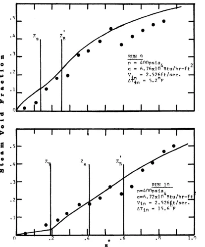
The effect of the inlet subcooling, ATj;^ pn the predicted void fraction

is shown in Figs. 5 and 4. and one can draw the following conclusions I

1. As the inlet subcooling is decreased, the subcooled boiling

length decreases,

2. The steady state vapour generation increases with decrease of

the inlet subcooling.

The effect of the system pressure is shown in Figs, 7 and 8, In Fig; 7

the subcooling.is less than that of Fig, 8, and thus the exit void

fraction should be higher than that of Fig, Q, However, the exit void

fraction in Fig, 8 is higher than that of Fig, 7» This indicates that

as the system pressure increases, the volumetric rate of steam genera

tion decreases.

Concluding, it should be noted that a number of assumptions were

made to simplify both the steady state and the unsteady state analysis.

Some of these assumptions are I

1, The effect of bubble condensation as the bubble is swept down

stream by the subcooled liquid was not included in this present analysis.

For very low inlet liquid flow rate, this effect may be important in

determining the void fraction in the subcooled boiling region and should

be accounted for. The experimental void data tested were obtained for

appreciably high liquid velocities. Consequently, this effect was

assumed negligible,

2. For the dynamic analysis an expression for the single phase

heat transfer coefficient that accounts for the void fraction distribution

must be employed. This variation of the heat transfer coefficient as

(51)

Although the agreement between the predicted cross-sectional

average void fractions and the experimental void data was good, it is

apparent that the present expressions employed to account for such

variables as wall voidage, and the slip ratio in the subcooled boiling

region are not satisfactory. The overall result will be much improved

if the exact forms of the wall voidage, the parameter e and the slip

ratio in the subcooled boiling region are known. These require

extensive accurately measured void fraction, quality, liquid phase velo

city and vapour phase velocity data in the subcooled boiling region

(52)

42

• ex <1" c • •

4*1 c cr c f l (I ex

p., C" >

CM CO 4J (13 <4-1

cd u P eu e •H U 03 P X P: rP w 03 X-C t'* P •H Pi

I

PC : 03 T ) C pC

-c • ui OC

C

03 IP

* 4J C' • ■4-1 C \0

m 4 -1 CM c e *

* <M m O' . Il

P-. c r >

4J P (0 ■p P C o

T-i CC

^ 03

OC P •H

s

(0 *H P P3 > U-s

i}.j

o

r -fO P 03 (C

^ PC

p (Ci •H

Pf "C (0 03

^ 'H n3 K O

c c;

s _ ^ 4-1

'W M-i tr.

Pj

PC

< PC u COp

(53)

ta

0

•*<

e et

u h

P a r a m e t e r s

p s A O b a r ,

q » b . 0 + 0 . 6 x 1 0 R t u / h r - f t

V i n = 3 . A P f t / s e c .

O

>

S

et

4» m

P a r a m e t e r s

p ■ A O b a r

q - 6. 3 ± 0 . 2 x l 0 ‘^ R t u / b r - £ t ‘

V i n ■ ' 3 . A 6 f t / s e c .

J

I

L

I

.

10

M o d e l

A Neal, v a r i a b l e g

R R a n k o f f ( J d n e s ) . c o n s t a n t e C R a n k o f f ( J o n e s ) , v a r i a b l e r

Fi%, 2. V o i d f r a c t i o n P r e d i c t i o n U s i n g t b e M o d i f i e d R o w r l n q ’s M o d e l

(54)

uu

q= 6.76x10 Rtu/hr-ft p= AnOpsia

Vjn = 7.526 ft/sec.

ATln = 5.2*T

d

e

o ct h k

R—

■d _{Rim q}

g*= 6.76x10 Btu/hr-ft p« AOOpsla

Vjj, = 2. 526ft/sec. AT, = 5.20R

e

a

«

»

OB

Z

Model A Rogers R Neal

I) March.-Hoglund K Bankoff (.Tones) R Bankoff(Neal & Zlvi) G Zuher.Stauh &

Rliwaard

3. _Comparismr _{C h r i s ^ n ^ ^ s % p e r l m e n t a l DatafRef. 2Q)}

(55)

- RUN 10

“ p » AOOpsia,

q = 6.76x10 Btu/hr-ft

Vin- 2.526ft/sec. ATin = 15.6°F

0

W

4#

RUN 10

p = AOOpsia,

q = 6.76x10 Btu/hr-ft

Vin = 2.526ft/sec. ATin = 15.6 F

*

Model

A Rogers B Neal

D March-Hoglund E Bankoff(Jones) F Bankoff(Neal & Zivi)

G Zuber,Staub &

Bijwaard

Fig. At. Comparison of C h r i s t e n s e n ’s Experimental Data (Ref. 29)