Development of an Intermediate DOF Vehicle Dynamics Model for Optimal Design Studies

(1)

Abstract

LOWNDES, ERIK MCKENZIE. Development of an Intermediate DOF Vehicle

Dynamics Model for Optimal Design Studies. (Under the direction of Dr. Joseph W.

David)

The demands imposed by the optimal design process form a unique set of criteria

for the development of a computational model for vehicle simulation. Due to the large

number of simulations that must be performed to obtain an optimized design the model

must be computationally efficient. A competing criterion is that the computational model

must realistically model the vehicle.

Current trends in vehicle simulation codes have tackled the problem of realism by

constructing elaborate full vehicle models containing dozens if not hundreds of distinct

bodies. Each body in a model of this type is associated with six degrees of freedom.

Numerous constraint equations are applied to the bodies to represent the physical

connections. While the formulation of the equations is not particularly difficult, and in fact

has been automated in several software packages, the resulting model requires a

considerable amount of computational time to run. This makes the model unsuitable for

the application of computational optimal design techniques.

(2)

demands of the optimal design process. These models typically use less than a dozen

degrees of freedom to model the vehicle. They do a good job of predicting the general

motion of the vehicle and they are useful as design tools but they lack the accuracy

required for optimal design.

A model that bridges the gap between these two existing classes of models and is

suitable for performing optimal design was developed. The model possesses twenty-eight

degrees of freedom and consists of eight bodies which represent the sprung mass, the rear

suspension, the left front spindle, the right front spindle, and the four wheels. A driver

control algorithm was developed which is capable of driving the car near its handling

limits. The NCSU Legends race car was modeled and an attempt was made to optimize

(3)

Development of an Intermediate DOF Vehicle

Dynamics Model for Optimal Design Studies

by

Erik M. Lowndes

A thesis submitted to the Graduate Faculty of North Carolina State University

in partial fulfillment of the requirements for the Degree of

Doctor of Philosophy

Department of Mechanical and Aerospace Engineering

Raleigh

1998

(4)

(5)

Biography

The author was born in Boulder, Colorado on March 21, 1968. He graduated first

from Oak Ridge High School, Oak Ridge, TN in 1986. He attended the University of

Illinois at Urbana-Champaign in 1986 as a Chancellor’s Scholar in the Campus Honor’s

Program. In January of 1990 he received his Bachelor of Science in Engineering Physics.

He continued his studies at the University of Illinois, receiving a Master of Science in

Physics in May of 1991. The author was married on June 23, 1991.

In the Summer of 1992 the author entered the Ph.D. program in the Department of

Mechanical Engineering at North Carolina State University, Raleigh, North Carolina. In

(6)

Acknowledgments

The author wishes to express his sincere appreciation to the chairman of his

advisory committee, Dr. Joseph W. David, for his patience, encouragement, advise and

support throughout this research. The author is also grateful to Dr. C. Tim Kelley, Dr.

Larry M. Silverberg and Dr. John S. Strenkowski for serving on the advisory committee.

Many thanks are also due to Dave Lewandowski and Mark Strohmeyer for their

support, encouragement, and ideas. Additional thanks are due to Mark Etheridge and

Jarno Kilian, who, in addition to their encouragement and valued input, loaned their

personal computers to the author for use as part of the PVM parallel processing network

used to generate the results in this thesis.

Finally, the author would like to express his gratitude to his family, and especially

to his wife Celeste and his son Mason, for their patient understanding, sacrifice and

(7)

List of Tables

1.1 Vehicle Model Degrees of Freedom ... 2

1.2 Computational Degrees of Freedom ... 3

1.3 Identification of the Sub-Terms in the Equations of Motion... 45

1.4 Organization of the Vehicle Model Derivations ... 46

3.1 Front Suspension Kinetic and Potential Energy Terms... 73

3.2 Wheel and Tire Rotational Energy Terms... 73

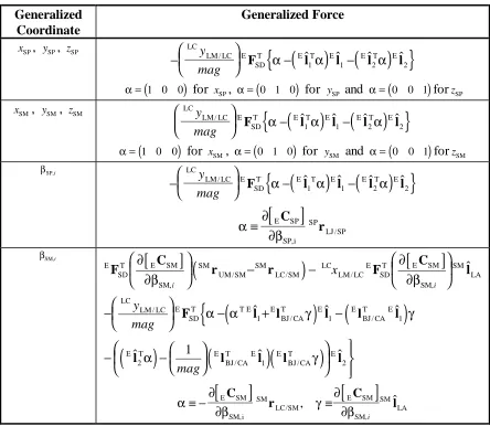
3.3 Generalized Forces due to Spring or Damper ... 74

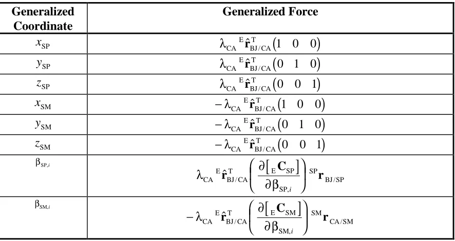
3.4 Generalized Forces due to the Control Arm Length Constraint... 75

3.5 Generalized Forces due to the Control Arm Orthogonality Constraint ... 76

4.1 Kinetic and Potential Energy Terms for the Motion of the Rear Suspension ... 86

4.2 Kinetic Energy Terms for the Rotation of the Rear Wheels and Tires ... 87

4.3 Generalized Forces Associated with a Rear Spring or Damper ... 87

4.4 Constraint Forces Associated with the Panhard Rod... 88

7.1 Desired Longitudinal Force Sign and Sign of the Longitudinal Slip... 124

9.1 NCSU Legends Car - Front Suspension Geometric Data... 151

9.2 NCSU Legends Car - Rear Suspension Geometric Data, Spring Data and Damper Data ... 152

9.3 NCSU Legends Car - Sprung Mass Geometric Data ... 153

9.4 NCSU Legends Car - Model Mass and Inertia Properties ... 154

(11)

9.6 Miscellaneous Tire Model Parameters: Geometric Data, Slip Equation

Parameters and Normal Force Characteristics ... 157

9.7 Delft ’97 Tire Model Parameters: Pure Longitudinal Slip Equation ... 158

9.8 Delft ’97 Tire Model Parameters: Pure Lateral Slip Equation ... 159

9.9 Delft ’97 Tire Model Parameters: Combined Slip Equations... 160

9.10 Driver Model Parameters ... 163

9.11 Vehicle Setup Parameters ... 164

9.12 Optimization and Cost Function Computation Parameters... 165

9.13 Vehicle Suspension Parameter Optimization Ranges ... 177

(12)

List of Figures

2.1 Earth Fixed and Vehicle Sprung Mass Coordinate Systems ... 48

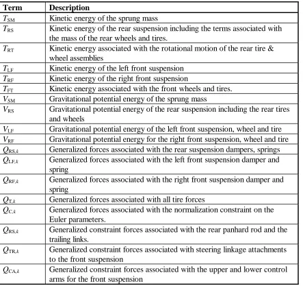
3.1 Schematic Showing Front of Sprung Mass and Control Arms ... 57

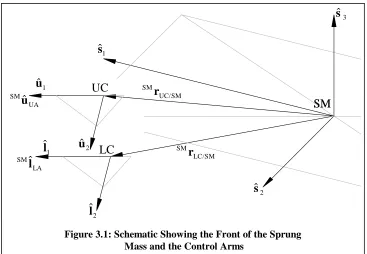
3.2 Schematic of Spindle and Control Arms ... 58

3.3 Schematic of a Generic Control Arm... 70

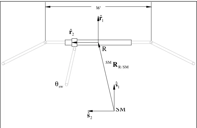
5.1 Schematic of the Rack and Pinion Steering System ... 90

5.2 Relationship between the P and S Coordinate Systems ... 91

5.3 Relationship between the D and P Coordinate Systems ... 92

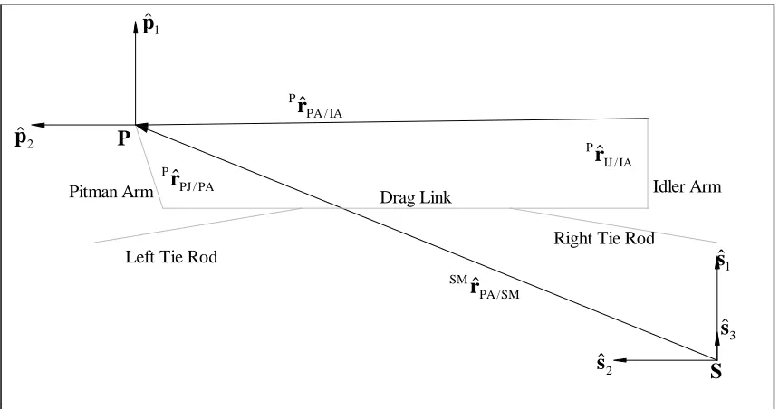
5.4 Schematic of the Four Bar Linkage Steering System ... 94

7.1 The Tire Model Coordinate System ... 118

7.2 Relationship between Tire Velocity Components... 123

8.1 Driver Path for the Kenley, NC Race Track ... 133

8.2 Steering Profile for the Kenley, NC Race Track ... 135

8.3 Driver Speed Controller Block Diagram... 139

8.4 Effect of the Traction Control Gain Parameter on the Acceleration ... 143

(13)

9.1 Schematic of the Kenley, NC Race Track... 161

9.2 Optimized Steering Profile for the Kenley, NC Simulation... 168

9.3 Optimized Velocity Profile for the Kenley, NC Simulation ... 169

9.4 Comparison of the Prescribed Velocity and the Actual Vehicle Velocity... 170

9.5 Vertical Acceleration of the Sprung Mass (Sprung Mass Coordinate System)... 171

9.6 Longitudinal Wheel Slip Percentages ... 172

9.7 Vehicle Position and 9.0 Seconds (Exiting Turn 2)... 173

9.8 Tire Normal Loads... 174

9.9 Vehicle Lateral Position Error... 175

9.10 Yaw Velocity... 176

(14)

1 Introduction

1.1 Motivation for the Study

The demands imposed by the optimal design process form a unique set of criteria

for the development of a computational model for vehicle simulation. Due to the large

number of simulations which must be performed to obtain an optimized design the model

must be computationally efficient. For a fixed execution time a faster simulation will, in

general, lead to a better design. A competing criteria is that the computational model

must realistically model the vehicle.

Current trends in vehicle simulation codes have tackled the problem of realism by

constructing elaborate full vehicle models containing dozens if not hundreds of distinct

bodies. Each body in a model of this type is associated with six degrees of freedom.

Numerous constraint equations are applied to the bodies to represent the physical

connections.1 While the formulation of the equations is not particularly difficult, and in fact has been automated in several software packages, the resulting model requires a

considerable amount of computational time to run. This makes the model unsuitable for

the application of computational optimal design techniques.

1

(15)

Past research in the field of vehicle dynamics has produced numerous

computational models which are small enough and fast enough to satisfy the speed

demands of the optimal design process. These models typically use less than a dozen

degrees of freedom to model the vehicle. They do a good job of predicting the general

motion of the vehicle and they are useful as design tools but they lack the required

accuracy for optimal design.

A model which bridges the gap between these two existing classes of models is

required for optimal design. This type of model combines element of both approaches to

obtain an accurate solution and yet still emphasize computational efficiency. This is the

type of model which is developed in this thesis. The model consists of eight bodies which

represent the sprung mass, the rear suspension, the left front spindle, the right front

spindle, and the four wheels. There are a total of twenty-eight dynamical degrees of

freedom which are distributed as shown in Table 1.1.

The total number of computational degrees of freedom is summarized in the Table

1.2. The equations of motion are second order which means that for each dynamical

degree of freedom there are two computational degrees of freedom (obtained in

Table 1.1 - Vehicle Model Degrees of Freedom

Body Degrees of

Freedom

Constraint Equations

Constraint Type

sprung mass 7 1 Euler Parameter normalization

rear suspension 7 5 EP norm, panhard rod, trailing links

front right suspension 7 5 EP norm, upper (2) and lower (2)

control arms

front left suspension 7 5 EP norm, upper (2) and lower (2)

control arms

(16)

converting the second order differential equations to pairs of first order differential

equations). The constraint equations introduce additional degrees of freedom in the form

of Lagrange multipliers which are necessary for determining the constraint forces. There

are a total of 80 computational degrees of freedom.

1.2 Historical Background

2

The study of automobile stability and control is a relatively new field. Although

significant quantities of automobiles were being produced in the early 1900s few efforts

were made to quantify the handling issues. Much of the early development was done on a

“cut and try” basis and this methodology is reflected in the literature. The majority of the

effort prior to 1925 was expended in designing suspensions which would keep the tires in

contact with the ground as much as possible in order to enable more effective steering

control. This preoccupation with controllability is typical of the early work. Progress in

the area of automotive stability was not seen until the 1930s.

2

Much of the historical information prior to the mid 1950s is from the following references: [ Segel, 1956a], [Milliken, 1956], [ Segel, 1956b] and [Whitcomb, 1956].

Table 1.2 - Computational Degrees of Freedom

Body Dynamical

Degrees of Freedom

Constraint Equations

Computational Degrees of

Freedom

sprung mass 7 1 15

rear suspension 7 5 19

front right suspension 7 5 19

front left suspension 7 5 19

wheels 4 none 8

(17)

In 1903 the Wright brothers successfully built their first airplane. In the same year

G. H. Bryan started his pioneering work on a mathematical theory of airplane stability

which was a few years later [Bryan, 1911]. While the refinement of Bryan’s stability

theory progressed steadily similar theories for the automobile didn’t appear until much

later. This delay was most likely due to the less pressing need to consider stability in

ground vehicles as compared to aircraft. The development of usable aircraft hinges on an

understanding of aerodynamics and how it affects the stability of an aircraft. This

understanding had been evolving with the use of scale models and wind tunnels. The slow

development of an automotive stability theory was also the result of a lack of

understanding of the role of the tire mechanics in the stability of an automobile.

The emphasis on vehicle control between 1900 and 1930 led to kinematic studies

of suspension and steering geometries. These studies led to improved designs including

Akermann steering geometry. Much of the remaining development work was concerned

with the drivetrain, structure and performance of the automobile with one notable

exception: A general theory of ride dynamics (the motion of the automobile in its plane of

symmetry) was well established by 1925. However, very little, if any, progress had been

made in the areas of static and dynamic directional stability. This statement may seem a

little strange at first given that the equations for ride dynamics are similar to those

involved in a full stability analysis. The key difference lies in the need to understand the

mechanism of lateral force generation by the tire. Without this knowledge it is impossible

(18)

In 1925 Broulheit published a paper in which the basic concepts of side-slip and

slip angle were recognized for the first time [Broulheit, 1925]. The recognition of these

concepts came about during attempts to explain the phenomenon of steering shimmy

which plagued vehicles of the time period. In 1931 Becker, Fromm, and Maruhn published

a text on the role of the tire in steering system vibrations and further developed the field of

tire mechanics [Becker, 1931]. This realization enabled further study of the problem of

automotive stability.

During the 1930s the Cadillac Suspension Group of General Motors, under the

direction of Maurice Olley, developed the first independent front suspension used on an

American car. It was found that certain steering geometries led to a condition which the

group termed oversteer [Olley, 1937]. It was recognized that these geometries led to

vehicles which were unsafe at high speeds. Olley’s oversteer is recognized today as being

roll oversteer. Further investigation revealed that behavior similar to oversteer could be

induced by over loading or under inflating the rear tires. In 1934 Olley wrote an

unpublished report containing his findings and in which the proposition of oversteer /

understeer was stated and the idea of critical speed was first mentioned [Olley, 1934]. As

a result of this research Goodyear Tire and Rubber Company began rolling drum tests to

determine tire characteristics and in 1935 R. D. Evans published the results in a paper on

lateral tire characteristics [Evans, 1935]. This paper gave data on cornering force and

self-aligning torque.

This work precipitated a period of extensive research at General Motors. The

(19)

exploration of steady-state tire characteristics occurred and skidpad tests were used for

the first time. A fundamental understanding of the steady state tire characteristics was

developed and a qualitative understanding of the transient behavior was obtained. During

the period from 1939 to 1945 very little progress was made due to World War II.

In 1950 Lind Walker summarized the current state of knowledge on the issue of

directional stability and introduced the concept of the ‘neutral steer line’ and the ‘stability

margin’ [Walker, 1950]. These concepts had already been established in aeronautical

circles and were suggested as criteria for steady state directional stability in automobiles.

The concept of using aerodynamics and tire characteristics to aid in achieving stability was

also proposed.

Vehicle Modeling

By the middle of the 1950s the groundwork for a mathematical model of the

vehicle had been laid. A basic understanding of the tire enabled the creation of reasonably

accurate mathematical tire models.

In 1956 William F. Milliken, David W. Whitcomb, and Leonard Segel of the

Cornell Aeronautical Laboratory, published the first major quantitative and theoretical

analysis of vehicle handling in a series of papers [Segel, 1956a][Milliken, 1956][Segel,

1956b][Whitcomb, 1956]. These papers formed the basis for research in the area of

automotive stability and control for the next three decades and are still frequently

(20)

Milliken’s paper [Milliken, 1956] provides a historical overview of the field from which

much of the above material was taken. In summarizing the progress made to date, Milliken

made the following statement,

Thus, [the] major effort in handling research to date has been in the recognition of individual effects, their isolation, and examination as separate entities. This work naturally started out as qualitative and in some instances has become quantitative. It has been conceptual in character; it has been pioneering and not infrequently intuitive and inspired, but it can hardly be viewed as an end in itself. Rather, it is a substantial beginning. All the individual effects now known need quantitative analytical expression. More significant, however, is the need for comprehensive, integrated analysis methods, for such overall theories will enable the prediction of the actual motion by rationally and simultaneously taking into account all of the separate effects.

Milliken also noted that, although a great deal of progress had been made in

understanding the tire, there was much to be done still. Although much has been learned

about tire modeling Milliken’s observation is still true today; dynamic data on tires is only

now becoming available. There were no universally accepted set of reference axes and

measured tire data of the period were typically confined to two or three of the possible six

force/moments. This made translation of the data from one set of axes to another difficult

if not impossible. It was also recognized that the effects of tire design on handling were

largely unknown and that there existed a need to perform testing on a wide variety of

common passenger car tires to determine the effects of the various design parameters. In

discussing of the future objectives of the Cornell Aeronautics Lab research program

(21)

control’. In the process he made the following distinctions between stability and control,

performance and ride.

In general, an automobile has ‘six-degrees-of-motion’ freedom, and stability and control may be thought of as those lateral motions out of the plane of symmetry involving rolling, yawing and sideslipping. (‘Performance’, by way of distinction, is concerned with fore-and-aft motions in the plane of symmetry, such as acceleration, speed, and braking, while ‘ride’ is composed of the vertical and pitching motions in the plane of symmetry.)

The second paper of the series, written by Leonard Segel, derives a set of

nondimensionalized linearized three degree of freedom equations for lateral and directional

motion [Segel, 1956b]. In accordance with the research goals outlined by Milliken the

emphasis of the model was put on modeling for analysis of stability and control. The

bounce and pitch degrees of freedom of the chassis were ignored and a fixed longitudinal

roll axis parallel to the ground was used. Segel also made several other simplifying

assumptions including constant forward velocity, fixed driving thrust divided equally

between the rear wheels, and that the lateral mechanical properties of the tires are

decoupled from the longitudinal mechanical properties at the speeds studied. The

unsprung mass was modeled as a single non-rolling lumped mass.

An experimental validation of the model was performed using a 1953 Buick Super

four-door sedan. The vehicle was put through both pulse steering input and step steering input

tests and the transient response for the three degrees of freedom included in the model

(lateral displacement, yaw and roll) were measured at a variety of constant forward

(22)

taken at 32 mph in a series of frequency response curves with the results showing good

correlation.

The final paper in the series, written by D. W. Whitcomb, draws a series of conclusions on

automobile stability and control using a two degree of freedom model (yaw and side-slip)

with experimentally determined parameters [Whitcomb, 1956]. Due to the lack of a roll

degree of freedom, Whitcomb was able to assume that the car has no width and that the

tires lay on the centerline of the vehicle (a “bicycle model”). A set of linearized differential

equations is derived using stability derivatives and the steady state and transient responses

are studied. In studying the yaw response of the vehicle at a constant vehicle side-slip

angle (same angle for both tires) he introduces the concept of the “static margin”.

The static margin is an indication of the sense and amplitude of the yawing moment associated with the total tyre side force. It immediately determines the yawing moment that the tyres would provide in reacting an externally applied side force.

In his summary of response characteristics Whitcomb recognizes the strong

influence of the static margin on vehicle stability. For vehicle with a negative static margin

it was recognized that a critical speed existed, which if exceeded, would lead to instability.

As noted by Milliken, there existed a need to quantify and refine the current knowledge of

the individual vehicle subsystems. Additionally, he recognized the need to combine these

refined models into improved full vehicle models. Progress towards achieving these goals

(23)

In 1960 H. S. Radt and W. G. Milliken Jr. explored the motions of a skidding

automobile [Radt, 1960a][Radt, 1960b]. They used a relatively simple vehicle model with

yaw and lateral velocity as the only degrees of freedom. A tire model was incorporated

which included the effect of saturation of the side force in the presence of braking and

thrust forces via the concept of a friction circle. Results were presented for a series of

steady state and transient maneuvers on a low friction surface (µ=0.3). A simple driver

control was also implemented to study skid recovery. The driver model was based on

feedback from heading angle with a first order lag. Results are presented for several gains

and lag time constants.

In August of 1961 Martin Goland and Frederick Jindra published a paper which

they used a two degree of freedom (yaw and sideslip) vehicle model to study the

directional stability and control of a four wheeled vehicle [Goland, 1961]. The model is a

simplified version of Segel’s model with the main difference being that the roll degree of

freedom enters as a quasi-coordinate which is only used to calculate the vertical load on

the tires. The paper takes into account the effects of load transfer and the variation of the

cornering performance of the tires with vertical loading. Results are presented which show

how the stability of a vehicle changes as the center of mass is moved, the tire inflation

pressure is changed, and the tire tread width is changed. The effect of tread width and

inflation pressure on the tire properties is given by a simplified form of the semi-empirical

equations published by R.F. Smiley and W. B. Horne in the late 1950s [Smiley, 1958].

Walter Bergman published a paper in 1965 in which he explored the nature of

(24)

established for steady state maneuvers, they were not well established for the transient

case. Bergman discussed the many origins of understeer and oversteer behavior including

steering inputs, aerodynamic forces and inertia forces in the transient case. He noted that

understeer and oversteer could be recognized by considering the change in the yaw

velocity induced by a change in lateral acceleration. This definition is in accordance with

the standardized definitions of oversteer and understeer put forth by the Society of

Automotive Engineers [S.A.E., 1965]. Bergman also develops a six degree of freedom

vehicle model to explore understeer and oversteer behavior as well as vehicle stability. The

model consists of a sprung mass and a single unsprung mass. The position of the unsprung

mass is given with respect to an inertial coordinate system by a two dimensional vector

and a yaw angle. The location of the sprung mass is given relative to the unsprung mass in

terms of four vertical wheel displacements. Both masses are assumed rigid which implies

that one of the vertical displacements is redundant.

In 1966 Segel published a paper in which the stability of a free control automobile

(i.e. a vehicle with torque input at the steering wheel as opposed to a steering angle input)

was studied [Segel, 1966]. He proposed a two degree of freedom quasi-linear (due to

Coulomb friction) model for the steering system. This steering model was added to his

three degree of freedom model which was discussed above. The model was validated by

comparing simulation output, performed on an analog computer, to experimental data. A

reasonably good correlation was demonstrated as long as the lateral acceleration of the

(25)

vibrational modes of the combined vehicle and steering model and to relate them to

vehicle design parameters.

In 1967 R. Thomas Bundorf of General Motors published a paper relating vehicle

design parameters to the characteristic speed and to understeer [Bundorf, 1967]. This

paper utilized the definitions of understeer and characteristic speed proposed by the SAE

publication Vehicle Dynamics Terminology [S.A.E., 1965]. Methods are proposed to predict understeer quality in vehicle designs and for measuring understeer in existing

vehicles. It is noted that the characteristic speed is an attribute associated with a linear

vehicle model. Bundorf argued that under most normal driving conditions, which he

characterized as having lateral accelerations below 1/3 g, a vehicle can be accurately

modeled by a linear model. This condition led to the construction of a large diameter skid

pad at GM for measuring the characteristic speed; it was not possible to reach high

enough vehicle speeds for accurate measurement of the characteristic speed on the

existing small diameter pad without exceeding the 1/3 g limit on lateral acceleration.

Bundorf derived an expression for predicting the characteristic speed of a vehicle given the

design parameters. The vehicle model used in his derivation was a bicycle model with

Ackermann (no slip) steering. The paper also contains a discussion, written by A. G.

Fonda, of Bundorf’s results with several significant contributions and suggestions.

D. H. Weir, C. P. Shortwell, and W. A. Johnson published a paper in 1968 which

they explored the role of vehicle dynamics on controllability [Weir, 1968]. Their results

were obtained using experimental data and simulation data obtained from a model which

(26)

and Segel’s earlier models. The model consisted of two unsprung masses representing the

front and rear suspension assemblies respectively and a single sprung mass representing

the body of the vehicle. The dynamics of the vehicle were described by a linearized set of

equations in four degrees of freedom (roll of the sprung mass about a fixed axis, lateral

velocity, yaw rate, and axial velocity). The three masses were assumed to posses the same

yaw rate, axial velocity and side slip velocity. Provisions were made for a stationary tilted

roll axis. In accordance with the inclusion of the axial velocity as a degree of freedom,

aerodynamic loads on the vehicle, longitudinal tire forces generated by braking and

acceleration and rolling resistance were considered. Dynamic data for a number of

automobiles made by U.S. manufacturers is also presented and, as an example, the transfer

functions for a typical 1960s sedan were calculated. It was noted that the yaw, lateral

velocity and roll modes have undamped natural frequencies of approximately 6 rad/sec at

60 mph. The yaw and lateral velocity modes are highly damped and the roll mode is lightly

damped. The roll mode damping ratio was found to be approximately 0.2 to 0.3 and it was

found to be largely decoupled from the yaw and lateral velocity modes. Increasing vehicle

speed tends to lower the vibrational frequencies and decreases damping which leads to a

destabilization of the vehicle.

By the early 1970s simulations of vehicle dynamics were becoming more complex

and realistic. This was primarily due to advances in computing technology. Prior to the

1970s most simulations were performed on analog computers. These machines were

capable of solving the vehicle dynamics problems in real time (since the differential

(27)

manner. Unfortunately it was very difficult to model nonlinear functions of more than one

variable on these machines. Since most tire models are nonlinear functions of more than

one variable the accuracy of the simulations was compromised by limitations in the

computing equipment. The advent of digital computers allowed researchers to create

models containing nonlinear functions. This allowed increased realism in the simulations,

however, the slow speed of the digital machines (typically 10 to 100 times slower than real

time) meant increased computing costs. In the early 1970s researchers designed simulation

codes which ran on hybrid computers which combined digital and analog computing

hardware [Murphy, 1970][Tiffany, 1970][Hickner, 1971]. The new computers made it

possible to run simulations at real time speeds and at the same time include nonlinearities

in the model. A number of papers on computing techniques and on models can be found in

the literature. A few of the more significant papers are discussed below.

In the early 1970s a vehicle dynamics simulation for a hybrid computer was created

by the research staff at the Bendix Corporation Research Laboratories [Tiffany, 1970].

The model was based on the ten degree of freedom model created by R. R. McHenry and

N. J. Deleys at the Cornell Aeronautics Laboratory for the Bureau of Public Roads

[McHenry, 1968]. The BPR-CAL model was improved by adding four spin coordinates

for the wheels and three coordinates for the steering system model. The original

BPR-CAL model had six coordinates for the sprung mass, one vertical coordinate for each front

wheel, and one vertical and one rotational coordinate for the rear axle. The steering

system model is based on Segel’s model [Segel, 1966]. At the time of publication the

(28)

model. The model was upgraded in 1971 to include a dynamically accurate model of a

four wheel anti-lock braking system [Hickner, 1971].

In 1973 T. Okada et al described in a paper a seven degree of freedom model for

vehicle simulation [Okada, 1973]. The model was used to simulate vehicle handling at the

first stage of vehicle design. Five of the degrees of freedom were used to model the

vehicle (roll, yaw, pitch, lift and lateral position). The remaining two degrees of freedom

were used to model the steering system in a manner similar to that proposed by Segel. The

vehicle was assumed to move with constant velocity. A tractive force was applied to

maintain constant vehicle speed and compensate for the six components of aerodynamic

forces which could be applied to the model. A roll axis which moves vertically in

accordance with the wheel travel was included. The effects of roll steer, axle steer, caster,

camber, toe-in, and so on were approximated by linear functions based on wheel travel,

steer angle etc. The simulation could be run in three different modes: straight-running

(with lateral “wind gust” disturbances), stationary circular motion (skid pad), and a slalom

mode (to predict critical speed). Gyroscopic effects of the wheels were only included in

the straight-running simulation mode where vehicle speeds are high. Steady-state motion

was assumed in the skid pad simulation which lead to simplification of the equations of

motion and an essentially algebraic system of equations for determining the maximum

lateral acceleration. For the slalom course simulation transients of the motion of the

vehicle were neglected and constant forward speed was assumed. The path followed was

assumed to be periodic with length 2*L where L was the distance between the cones.

(29)

speed at which a solution could no longer be obtained. Driver response time limitations

were considered as well as vehicle limitations in determining the critical speed.

In 1973 Frank H. Speckhart published a paper in which he presented a vehicle

model containing fourteen degrees of freedom [Speckhart, 1973]. Six degrees of freedom

were assigned to the sprung mass, four degrees of freedom were associated with the

suspension movement at the four corners of the vehicle, and four rotational degrees of

freedom were assigned to the wheels. He used a Lagrangian approach in deriving his

equations. Models were presented for several different suspension configurations. The

sprung mass was restricted to pivot about a specified roll axis. It is likely that this is done

because the suspension models were relatively simple (two dimensional in the case of the

front independent suspension) and did not provide a sufficiently accurate representation of

the kinematics involved.

As digital computers gradually displaced analog and hybrid machines, primarily as

a result of economic concerns, it became necessary to create vehicle dynamics models

which were completely digital. The combination of the cost of computer time and the

slower solution speed of the digital machines made it desirable to create computationally

efficient models.

In 1973 Bernard published a paper detailing several time saving methods used in

the digital vehicle simulation code created for the Highway Safety Research Institute

[Bernard, 1973]. He noted that the important sprung mass motions tended to be in the low

frequency range (below 2 Hz) and that the significant wheel hop motions tended to be

(30)

with a relatively large time step (0.005 sec) and obtain accurate results. Unfortunately the

cycling of brake torque (as in an anti-skid system) could cause rapidly changing spin

derivatives for the wheel degrees of freedom. The relatively high frequency motion

required a much smaller time step on the order of 0.0001 second. Bernard proposed an

approximate method for dealing with the spin degrees of freedom which allowed the use

of the larger time step. This improvement in combination with the use of a specially

modified predictor-corrector integration scheme which only updated the wheel-hop

derivatives during the corrector phase led to a speed improvement of a factor of five.

In early 1976 Frederick Jindra published an interim report for the NHTSA

describing a vehicle simulation model being created at John’s Hopkins University Applied

Physics Laboratory [Jindra, 1976]. The model was called the Hybrid Computer Vehicle

Handling Program (or HVHP) because it was run on a hybrid computer. The HVHP

model was derived from a refined version of the Bendix Research Laboratories (BRL)

model which was discussed above. The HVHP model was used extensively by Calspan in

their study on the influence of tire properties on passenger vehicle handling. The HVHP

model contained seventeen degrees of freedom distributed as follows: six for the sprung

mass, one for the vertical motion of each front wheel, two for the vertical motion and

rotational motion of the rear axle assembly, three for the steering system, and four

rotational degrees of freedom for the wheels. The program had an option to use an

independent rear suspension model. In this case the model contained two degrees of

freedom for the vertical displacements of the rear wheels. The steering system model was

(31)

front wheels about their steering pivots and one degree of freedom for the translational

motion of the connecting steering rod and associated mass elements. Friction and

compliance in the steering mechanism were included. The rear unsprung mass was

assumed to pivot about a point which was constrained to move along the sprung mass

vertical axis. This constraint was an improvement over the traditional fixed pivot point and

fixed roll axis. No pivot point was assumed for the independent front suspension; the front

wheels were assumed to move vertically with respect to the sprung mass. Due to the

difficulty in representing nonlinear functions on the hybrid machine, piecewise linear

functions were used to describe the spring force, coulomb friction, damping coefficients,

roll stiffness, etc. The camber angle, caster angle, and toe angle were specified as

functions of the suspension deflection. Compliance coefficients were used to model the

change in camber angle and steer angle due to applied forces and moments at the tire.

Radial loading of the tire was computed using a point contact model.

In 1977 Kenneth N. Mormon of Ford Motor Company presented a paper

[Morman, 1977] containing a detailed three degree of freedom model of the front

suspension. The model included the effects of lower control arm bushing compliance along

the axis of rotation (but not perpendicular to the axis of rotation) and compliance of the

ball joints connecting the tie rod ends to the steering knuckle. The model was derived

using a standard Lagrangian approach with constraint equations. A variety of displacement

type inputs were applied to the model; the results of the simulation matched experimental

results fairly well. In the original model all of the spring, dampers and bushings were

(32)

with appropriate nonlinear relations. It was also assumed that the sprung mass of the

vehicle forms inertial coordinate system.

In 1981 W. Riley Garrot described an all digital vehicle simulation developed at the

University of Michigan [Garrot, 1981]. The model contained a total of seventeen degrees

of freedom distributed in a manner identical to the HVHP model discussed above. To

reduce computational costs the steering system was described statically and the wheel-spin

degrees of freedom were handled algebraically. The model contained numerous features

which could be turned on or off as desired. These features included an anti-lock braking

system, multiple tire models, optional activation of nonlinear kinematic terms, solid rear

axle or independent rear suspension and interactive capability. The program was

constructed in a modular fashion to enable future enhancements and upgrades. The

simulation consisted of two main parts: a vehicle model called IDSFC and a

general-purpose driver module called DRIVER. The driver module could be readily altered

without affecting the vehicle model. The driver model controlled steering, braking and

drive torque inputs to the vehicle model. It contained five preprogrammed open-loop

maneuvers and could accept user defined maneuvers using tabulated data or a user defined

subroutine. Various closed-loop control strategies were implemented including a

crossover model for path following and two types of preview-predictor models. Mixed

open-loop and closed-loop control could be used. Validation of the model was performed

by comparison with the validated HVHP model.

In 1986 R. Wade Allen and several associates from Systems Technology Inc.

(33)

validate a simplified lateral vehicle dynamics model and the associated tire modeling

procedure [Allen, 1986]. The tests consisted of a number of steady state skid pad runs and

several low amplitude sinusoidal steer frequency sweeps while negotiating a steady turn.

The tests were performed for a rear wheel driver 1980 Datsun 210 and a front wheel drive

1984 Honda Accord. Several types of tires were used on the Datsun including both radial

and bias ply tires. The physical parameters describing the vehicles and the tires were input

into a simplified lateral handling model which was derived directly from Segel’s original

model [Segel, 1956b] and which was discussed above in the review of D. H. Weir’s paper

[Weir, 1968]. A good correlation was obtained with the experimentally obtained data. The

model was also used to extrapolate vehicle behavior under combined cornering and

braking. In 1987 Allen published a revised model containing five degrees of freedom

[Allen, 1987a]. The new model added pitch and forward velocity degrees of freedom and

was called VDANL (Vehicle Dynamics Analysis : Non-Linear). It was also a nonlinear

model and, unlike earlier linear models, the solutions were obtained in the time domain

using numerical integration. Neither of the models approach the complexity of some of the

other more detailed models discussed above [Okada, 1973][Speckhart, 1973][Jindra,

1976]; the intent was to provide a simulation code which could be run on relatively

inexpensive desktop PCs and which could utilize the graphical output capabilities of those

PCs.

In 1987 Andrez Nalecz presented the results of an investigation into the effects of

suspension design on the stability of vehicles and, in particular, how the design of the

(34)

suspension types were considered. A typical three degree of freedom lateral dynamics

model was used with the addition of a quasi-static pitch degree of freedom. The sprung

mass was assumed to rotate about a roll axis whose position varied as a function of body

roll. The location of the front and rear roll centers was found via a kinematic analysis of

the suspension in which the wheel contact patches were treated as revolute joints and were

allowed to move laterally along the ground (thus allowing for track width changes). It was

found that for certain types of suspensions, most notably the double wishbone and

MacPherson strut type systems, that the assumption of a fixed roll axis could not be

justified. In 1992 Nalecz published a second paper in which he described an eight degree

of freedom model called LVDS (Light Vehicle Dynamics Simulation) [Nalecz, 1992]. The

model consisted of a three degree of freedom lateral dynamics model coupled to a five

degree of freedom planar rollover model. The models are coupled through the inertia

terms and tire force terms. The lateral dynamics model was derived in the same manner as

Segel’s original model. The rollover model consisted of sprung and unsprung masses

connected through the various elements of the suspension system. The model also

included aerodynamic effects; all six possible forces and moments are modeled. The effects

of lateral and longitudinal weight transfer were accounted for in determining the lateral

forces generated by the tires. The roll axis was modeled in the quasi-static fashion

discussed above.

In the early 1990s R. Wade Allen and his associates at Systems Technology Inc.

published a number of papers in which they validated their VDANL simulation code

(35)

of vehicle stability and vehicle rollover are presented [Allen, 1990][Allen, 1991][Allen,

1993]. VDANL and IDSFC (which is derived from the HVOSM simulation code) were

also put through a rigorous validation process by Gary J. Heydinger et al at Ohio State

University [Heydinger, 1990]. Both validations were carried out by comparing

experimental data to simulation data in the time domain and in the frequency domain. The

control inputs from the experimental tests were recorded along with the vehicle responses

for later use as simulation inputs. Sinusoidal frequency sweeps and step inputs were used

in the testing. Heydinger explored the use of pulse inputs which require shorter test runs

and could excite the same frequency range in a later paper [Heydinger, 1993]. In studying

vehicle stability and rollover stability the authors gathered model parameter data for a total

of 41 different vehicles of various types. The connection between load transfer distribution

(which is largely governed by the relative roll stiffness at the front and rear axles) and

vehicle stability was discussed in detail. Simulation results for a set of maneuvers were

plotted. The effects of braking, acceleration and throttle lift on stability in limit handling

situations was also discussed. A similar paper, also using the VDANL software, was

written by Clover and Bernard at Iowa State [Clover, 1993]. Details of the updated

vehicle dynamics model VDANL were presented in [Allen, 1991]. The biggest change in

the model was the removal of the fixed roll axis assumption and the addition of a front

suspension model which reflects camber change with body roll. The model also included

the effect of lateral deflection of the tire, wheel and suspension which decreases the track

width and affects rollover stability. In [Allen, 1993] the authors demonstrated that the

(36)

studies in that it failed to cause unstable behavior and that it did not adequately model the

large lateral displacements which could occur in real world accident avoidance maneuvers.

Simulation results for larger lateral displacements (with the same peak lateral acceleration)

demonstrated both spinout and rollover.

By the early 1980s a shift in the vehicle modeling process was taking place. The

demand for accurate vehicle dynamics models combined with the difficulty in deriving the

equations of motion for large multibody systems led to the use of general multibody

simulation codes. A wide range of capabilities are present in modern MBS codes including

the ability to handle non-inertial reference frames, to incorporate flexible elements in the

model, to utilize generalized coordinates, and to symbolically generate the equations of

motion. Several reviews of multibody codes have been published in recent years, several of

which are discussed in more detail below. Additionally, brief descriptions of a few papers

utilizing MBS codes for vehicle dynamics simulations are presented below.

In 1985 W. Kortüm and W. Schiehlen presented a paper [Kortüm, 1985] which

they presented the desirable qualities of an MBS program, discussed two contemporary

examples in some detail and utilized the two codes to generate some simple vehicle

models. The first code discussed was NEWEUL which generates the equations of motion

in symbolic form with the output being FORTRAN code. It had the capability of using

both Cartesian and generalized coordinates, non-holonomic constraints and moving

reference frames. The second program was MEDYNA which generates the equations of

(37)

moving reference frames. Both codes supported the use of closed loops (i.e. four bar

linkages).

In 1993 W. Kortüm and R. S. Sharp published a supplement to the periodical

Vehicle System Dynamics in which the capabilities of 27 currently available multibody simulation codes and general purpose vehicle simulation codes were reviewed [Kortüm,

1993]. The programs discussed include ADAMS, MEDYNA, NEWEUL, DADS,

AUTOSIM, and SIMPACK among others. Tables were presented which offer

comparisons of the capabilities of the various codes. Kortüm discussed the desirable traits

of a multibody code and gave a brief discussion of the contemporary numerical methods

which are most applicable to vehicle dynamics simulation. Sharp discussed the four models

which were used in benchmarking and evaluating the codes in his introduction.

In 1994 R. S. Sharp wrote a paper in which he compared the capabilities of the

major multibody computer codes with emphasis on those which generate the equations of

motion symbolically [Sharp, 1994]. The codes reviewed were selected based on their

applicability to automotive simulation. He discussed the methods used by each code in

deriving the equations of motion with attention to the limitations of each method. In

particular he noted the limitations of each code with respect to the types of constraint

equations that could be handled. References to significant papers in the area of multibody

dynamics were given.

R. J. Antoun discussed a vehicle dynamic handling computer simulation created

using the multibody code ADAMS (Automatic Dynamic Analysis of Mechanical Systems)

(38)

pickup truck was created utilizing a combination of the standard ADAMS model definition

language and user written subroutines for non-standard system components such as the

tires. A detailed kinematic model of the front I-beam suspension and the rear leaf spring

suspension (using a three link approximation) was constructed. The effects of bushing

compliance were included in the model. Nonlinear shock absorbers were used. Excellent

agreement of simulation results with experimental data was obtained. Other studies were

made using models for a 1986 Bronco II and a 1986 Aerostar van. Using the respective

models the researchers were able to optimize the stabilizer bar dimensions and tire

characteristics at an early stage of the design process. The Bronco model contained 55

degrees of freedom. It was noted that the extensive graphical display capabilities of the

ADAMS program were invaluable in debugging the model geometry and in interpreting

the results.

A paper describing a model built utilizing a program which automates the

generation of the equations of motion was presented in 1991 by C. W. Mousseau

[Mousseau, 1991]. The program, AUTOSIM, was used to create a 14 DOF vehicle

model. The program used a form of Kane’s equations to derive the equations of motion

and applies extensive algebraic and programming optimizations to achieve high efficiency.

The user was responsible for choosing the generalized coordinates which describe the

configuration of the system. It was not necessary to use Cartesian coordinates and

numerous constraint equations to formulate the equations of motion. In generating the

vehicle model the location and orientation of the spindle was expressed in terms of four

(39)

polynomial functions of the suspension deflection (a quasi-static approximation). The

cubic polynomials were obtained from a kinematic suspension model. The effects of

suspension geometry and suspension bushing compliance were included in the suspension

model which was also created using AUTOSIM. Integration of the resulting FORTRAN

model produced good correlation with measured data. The computational efficiency of the

resulting model allowed it to be used in real time in a driving simulator. In 1993 Michael

W. Sayers published a paper in which AUTOSIM was used to generate a number of

vehicle models [Sayers, 1993]. The simplest model possessed 4 degrees of freedom system

while the more complicated models contained 10 degrees of freedom. The emphasis in the

paper was on demonstrating the ease with which computationally efficient models can be

generated and tested.

Yoshinori Mori et al at Toyota described a model created for simulation of active

suspension control systems in a paper presented in 1991 [Mori, 1991]. The vehicle model

was described using a simulation language. The control algorithms were coded in

FORTRAN and interfaced to the vehicle model. The vehicle model contained 20 degrees

of freedom. The unsprung masses were assigned three degrees of freedom each and the

sprung mass was given six degrees of freedom. Each of the front wheels was assigned a

single steer degree of freedom. The model also included a 19 degree of freedom

drive-train model. Provisions for front wheel drive, rear wheel drive and four wheel drive were

made. The road surface was modeled using a combination of a flat or undulating surface

(40)

In 1989 a research group at the University of Missouri-Columbia began a DOT

sponsored project to study the effects of vehicle design on rollover propensity [Nalecz,

1988]. A nonlinear 14 degree of freedom vehicle model called the Advanced Dynamics

Vehicle Simulation (ADVS) was developed to carry out this research. The model was

derived using a Lagrangian approach and utilizes quasi-velocities to describe the angular

velocities. The degrees of freedom were utilized as follows: three translational and three

rotational for the sprung mass, two for the front suspension and two for the rear

suspension and one rotational for each wheel. To study vehicle-terrain interaction it was

necessary to model the body of the vehicle as well as the terrain [Lu, 1993]. The vehicle

body was represented by a set of massless, three-dimensional nodes which obey nonlinear

force-deflection curves. Each node was checked for interference with the terrain at each

time step of integration and its position was adjusted as necessary. The force resulting

from body-terrain interaction was applied to the vehicle dynamics model. The terrain was

modeled by a single curve which was extruded along the direction of travel. This

prevented the use of curved roadways and other such fully three-dimensional structures

but it simplified the body node-terrain interference calculation substantially.

In 1993 the results of a program at Lotus Engineering to develop a vehicle

simulation code for studying the application of predominantly linear control algorithms to

the suspension of a nonlinear vehicle were published by J. G. Dickinson and A. J. Yardley

[Dickison, 1993]. Although commercial multibody simulation codes were available it was

desired to utilize a simpler model which did not require the large quantities of descriptive

(41)

paper utilized six degrees of freedom for the sprung mass. The front and rear suspensions

were modeled in a quasi-static fashion. Each wheel was assigned a ‘bump’ degree of

freedom which was measured relative to the sprung mass. The location of the

instantaneous pivot axis was determined from a look-up table based on the value of the

bump variable. Since the motion was handled in a quasi-static fashion the pivot axis

location, camber angles, wheel hub location, toe angle, effective spring rate, effective

damper velocities and so on could be calculated off-line. The front suspension was

modeled in the same fashion but adds a steering swivel axis and two degree of freedom

steering system. The tires were modeled using the Pacejka curve fits to measured tire data.

The longitudinal force at the tires was set by the driver acceleration input. The lateral

force was reduced accordingly by utilizing a standard friction ellipse. Wheel angular

velocities were apparently not included as degrees of freedom in the model. The authors

claimed a speed advantage of a factor of three over more complicated models generated

using standard multibody codes and hoped to increase the advantage to a factor of six in

later versions of the software.

In 1996 Michael R. Petersen and John M. Starkey described a relatively detailed

straight line acceleration vehicle model for predicting vehicle performance [Petersen,

1996]. The model included longitudinal weight transfer effects, tire slip, aerodynamic

drag, aerodynamic lift, transmission and driveline losses and rotational inertias of the

wheels, engine and driveline components. A manual transmission was assumed with 100%

clutch engagement. Shifts were simulated by disengaging the clutch completely, assuming

(42)

the full torque of the motor. Shifts occurred when the applied torque at the rear wheels in

the next gear exceeded the torque at the rear wheels in the current gear, or alternatively,

when redline was reached. After validating the model the authors conducted sensitivity

analyses to determine which design parameters most strongly affected vehicle

performance.

Driver Modeling

Beginning in the early 1960s an increasing emphasis on vehicle safety created a

push toward modeling vehicles under the more demanding conditions associated with

crash avoidance maneuvers. In order to accurately represent the reactions of the vehicle

under these circumstances it was necessary to include the driver as an integral part of the

model. While this fact had been recognized in the early 1960s it was not until the late

1960s that increasing computational power and an improved understanding of vehicle

dynamics and driver behavior made it practical to model the driver and vehicle together.

In 1968 David H. Weir and Duane T. McRuer of Systems Technology Inc.

published the first in a long series of papers on modeling driver steering control (lateral

control) [Weir, 1968b]. The vehicle dynamics were modeled using Segel’s equations

[Segel, 1956b]. The equations were Laplace-transformed and the analysis was performed

in the frequency domain. The transfer functions relating the motion variables to the inputs

were taken from Weir’s earlier paper [Weir, 1968a]. Although Segel’s steering system

model was available [Segel, 1966], the lack of dynamic data on vehicle steering systems

(43)

system dynamics. The driver model was divided into four subsystems: quasi-linear

compensatory control, pursuit control, precognitive control and a remnant.

The quasi-linear compensatory control consisted of a describing function with

parameters which were adjusted to fit the situation and the system, an additive remnant

and a set of adjustment rules. The form of the driver model, of the describing function and

of the parameter adjustment rules was derived from extensive experiments involving

human operators. It was noted that the parameter adjustment rules could be eliminated by

considering the combined response of the vehicle/driver system. In this case an approximate crossover model was found to represent driver/vehicle behavior adequately.

This simplification was a result of experimental studies involving human drivers which

found that drivers adjust their behavior to obtain an approximately invariant form for the

combined vehicle-driver response function.

The pursuit control subsystem modeled the driver’s ability to see the roadway

ahead. This is in contrast to the compensatory subsystem in which the driver reacted to

errors in the current position of the vehicle. The details of pursuit control are not

mentioned except to note that experimental evidence indicates that the magnitude of the

feedforward describing function was approximately equal to the inverse of the magnitude

of the vehicle response function. Thus the command path and the actual vehicle path are

nearly identical. It was also noted that compensatory control was often used in

combination with pursuit control to regulate errors in path following.

The precognitive control model attempted to mimic learned driver responses. A

(44)

another automobile. Weir and McRuer note that these types of maneuvers do not involve

a feedback based on position information or a feedforward based on the desired path. The

maneuver is initiated by the driver in response to stimuli other than those involved in

pursuit and compensatory control. No other results are presented by Weir and McRuer

beyond defining the nature of precognitive control.

The driver remnant component of the model accounted for the portion of the

driver’s output which was not linearly correlated with the input. It was modeled as a

random input which was described by an experimentally obtained power spectral density.

It was noted that the major source of this remnant is due to variation of the parameters of

the driver describing function. The remnant could be neglected for vehicles which

demonstrated good response characteristics.

Following discussion of the various model components them authors presented the

results of a guidance and control analysis of the potential loop closures for compensatory

control. A number of multiloop structures were considered. The best multiloop feedback

structures were considered to be those which demonstrated good frequency response and

required minimal driver attention. Based on the author’s analysis it was concluded that a

feedback structure based on heading angle and lateral acceleration gave the best results. A

review of perceptual experiments performed by other authors [Gordon, 1966a][Gordon,

1966b][Crossman, 1966] corroborates Weir and McRuer’s conclusions.

In a later paper Weir and McRuer reviewed data from experiments on the

directional response of vehicles subjected to cross wind gust disturbances. Driver/vehicle

(45)

McRuer’s earlier assertion that the driver’s steering outputs could be explained as

functions of lateral position and heading angle or alternatively as functions of path angle

and path rate.

In 1975 Errol R. Hoffman presented a paper [Hoffman, 1975] in which he

reviewed the state of the knowledge of human control of road vehicles. He covered lateral

control and longitudinal control of automobiles and motorcycles. The areas of research

reviewed in the paper were divided into the following major categories: lateral control of

automobiles, lateral control of motorcycles, longitudinal control of automobiles and

combined lateral and longitudinal control. The relevant portions of Hoffman’s review of

the literature in the areas of lateral and longitudinal control of automobiles is summarized

below. The work done in the area of lateral control was divided it into four sub-groupings:

lateral control vehicle dynamics, perceptual studies, mathematical models of driver

steering control and vehicle characteristics and driver/vehicle performance.

Hoffman classified the work done on lateral control vehicle dynamics category into

the following three categories: fixed control, free control and vehicle-driver interface

variables. Fixed control occurs when steering wheel input angle is specified directly. Free

control occurs when the steering wheel input is in the form of a specified torque. The

majority of the research up to the time of publication of Hoffman’s review had been

performed on the fixed control mode; very little work had been performed using free

control. Hoffman noted that, in reality, a human driver uses a combination of the these

two types of control. He also noted that the proportion of each type of control varies with

(46)

vehicle dynamics category encompassed research done on driver/vehicle interface

variables. Driver/vehicle interface variables are defined as the quantities which relate

steering wheel input (either angle or torque) to vehicle response. Typically they are

approximations to the actual output and are used in determining gains in the control

algorithms. Again, the majority of the existing work concentrated on identification of the

gains associated with fixed control (i.e. neutral steer path curvature vs. steering wheel

angle, etc.). Very little work had been performed relating steering force to vehicle

response for the free control mode.

At the time of Hoffman’s review a number of papers on driver perception of the

roadway had been published. Several papers suggested that the driver uses the perceived

velocity field to guide the vehicle. Later studies of driver eye movements indicated that

peripheral vision is used to monitor steering control for tracking and directional guidance

while central vision is used for obstacle avoidance. Studies of driver steering control

movements indicated that vehicle yaw rate and inertial lateral deviation are the most

probable control cues used by the driver.

Hoffman reviewed a variety of mathematical models available in the literature at

the time. He included a brief review of the quasi-linear model proposed by McRuer et al

which was discussed in above. He also briefly discussed the predictive models of Kondo

and Ajimine and of Yoshimoto [Kondo, 1968][Yoshimoto, 1969]. These models were

single loop models which used estimated position and heading data as feedbacks. Hoffman

also mentioned an optimal control model outlined by Roland and Sheridan [Roland,