Development of Machine Learning Methods for Turbulence Combustion Closure and Chemistry Acceleration.

(1)

ABSTRACT

RANADE, RISHIKESH. Development of Machine-learning Methods for Turbulence Combustion Closure and Chemistry Acceleration. (Under the direction of Dr. Tarek Echekki).

Turbulent combustion involves complex interactions between turbulence and chemistry. These interactions result in several turbulent combustion phenomena occurring in different combustion applications. Due to the massive complexity involved, turbulent combustion requires modeling for accurate prediction and representation of these phenomena; and the models developed in this respect are conventionally known as turbulent combustion closure models. The objective of this work is to explore data-based and machine-learning techniques to enable the construction of new closure models and improve the existing ones.

(2)

scalars, density and PC source terms to determine their unconditional means. These means are represented in terms of mean PCs using artificial neural networks (ANN). The closure model based on experimental measurements is validated using a priori and a posteriori tests. In the a priori analysis, the reconstructed mean and RMS statistics of thermo-chemical scalars for two flames, the Sandia piloted jet diffusion flames and the Sydney piloted jet flames with inhomogeneous inlets, are in excellent agreement with their respective experimental means. Additionally, the a priori analysis also includes a demonstration of source term reconstruction using the modified PMSR approach. In a posteriori analysis, the closure framework is validated by performing RANS calculations for the Sandia piloted jet flames and the Sydney piloted jet flames with inhomogeneous inlets. The axial and radial profiles of mean temperature, mixture fraction and measured species mass fractions agree well with the experimental means for these flames.

(3)

(4)

(5)

Development of Machine-learning Methods for Turbulence Combustion Closure and Chemistry Acceleration.

by

Rishikesh Ranade

A dissertation submitted to the Graduate Faculty of North Carolina State University

in partial fulfillment of the requirements for the degree of

Doctor of Philosophy

Mechanical Engineering

Raleigh, North Carolina 2019

APPROVED BY:

_______________________________ _______________________________ Dr. Tarek Echekki Dr. Alexei Saveliev

Committee Chair

(6)

ii

DEDICATION

This dissertation is dedicated to my beloved and dear friend Ansal George.

(7)

iii

BIOGRAPHY

(8)

iv

ACKNOWLEDGMENTS

I would like to take this opportunity to thank Dr. Tarek Echekki for his immense support, patience and guidance through the 4 years of my PhD. His continuous encouragement has pushed me to strive harder and to become a better researcher. I would like to acknowledge Dr. Alexei Saveliev, Dr. Tiegang Fang and Dr. Phillip Westmoreland for serving on my PhD committee. They have been very encouraging and supportive during different phases of my PhD career. I would also like thank my lab mates, Dr. Opeoluwa Owoyele and Sultan Alqahtani for the good times we spent, in and outside of our lab. I wish them the best of luck in their future endeavors.

During my PhD, I had the privilege of collaborating with the reacting flow development team at Ansys Inc. My appreciation goes to, Dr. Ellen Meeks, Dr. Shaoping Li, Dr. Genong Li, Dr. Rakesh Yadav and Dr. Hossam El-Asrag. I have learnt a lot from them regarding combustion modeling and computational fluid dynamics.

(9)

v

LIST OF TABLES

Table 3.1. Velocity information of the Sandia flames ... 60

Table 3.2. Thermo-chemical composition of pilot. Flame F temperature is 1860 K. ... 61

Table 5.1. Memory storage comparison. ... 193

Table 5.2. Scalars in different groups using clustering. ... 195

Table 5.3. Average neurons/layer observed in A, B and C. ... 197

Table 5.4. RMSE for different scalars with number of clusters. ... 201

(13)

ix

LIST OF FIGURES

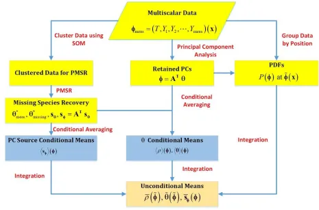
Figure 2.1. Flow chart of closure approach ... 34

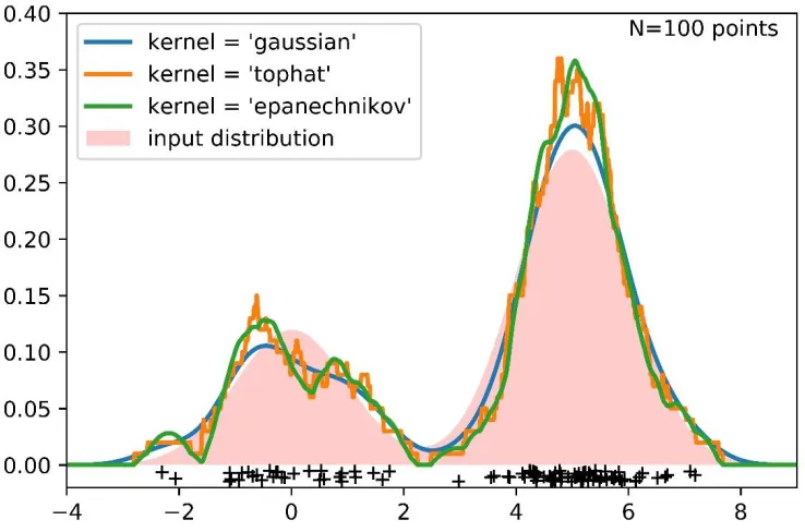
Figure 2.2. KDE estimation using different kernel functions for a bandwidth of 0.5 ... 42

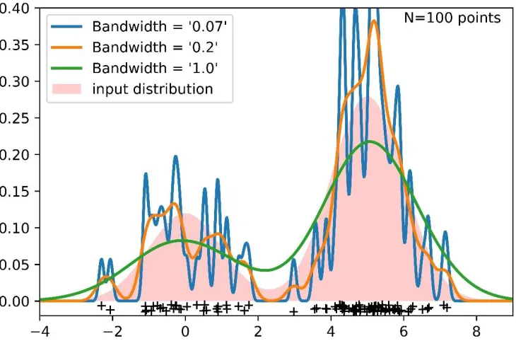
Figure 2.3. KDE estimation using different bandwidths for a Gaussian kernel ... 43

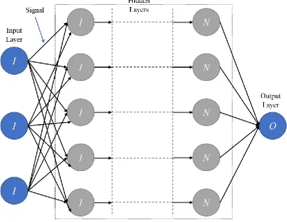
Figure 2.4. Artificial neural network architecture ... 50

Figure 3.1. A priori test procedure. ... 57

Figure 3.2. The Sandia Piloted jet burner (http://www.ca.sandia.gov/TNF/DataArch/FlameD.html) ... 62

Figure 3.3. Scree plot for the Sandia piloted flames D, E and F... 64

Figure 3.4. Correlations of leading 4 PCs vs mixture fraction for flame F. ... 65

Figure 3.5. Correlations of leading 4 PCs vs temperature (reaction progress) for flame F. ... 66

Figure 3.6. PC-distribution on the 2D SOM lattice. ... 71

Figure 3.7. Temperature, H2, CO and OH distribution in different clusters ... 71

Figure 3.8. Conditional source term comparison of PMSR reconstruction (left) and ODT (middle) for T, O2, H2O, CH4 and CO2. ... 73

Figure 3.9. Conditional source term comparison of PMSR reconstruction (left) and ODT (middle) for H2, CO and OH. ... 74

Figure 3.10. Conditional statistics of T, CH4, O2, H2O. ... 76

Figure 3.11. Conditional statistics of OH, CO, H2, CO2. ... 77

Figure 3.12. Joint PDFs for flame D (A, B) at r/d = 0 and x/d = 15, 30. ... 79

Figure 3.13. Joint PDFs for flame E (C, D) at r/d = 0 and x/d = 15, 30. ... 80

Figure 3.14. Joint PDFs for flame F (E, F) at r/d = 0 and x/d = 15, 30. ... 81

Figure 3.15. Flame D Favre averages (solid) and RMS (dashed) comparisons of experimental data (red) and PCA-based closure model with 2 PCs (black) at A) x/d = 7.5, B) x/d = 15, C) x/d = 30 and D) x/d = 45. ... 83

(14)

x Figure 3.17. Flame F Favre averages (solid) and RMS (dashed) comparisons of

experimental data (red) and PCA-based closure model with 2 PCs (black) at A) x/d = 7.5, B) x/d = 15, C) x/d = 30 and D) x/d = 45. ... 85 Figure 3.18. Flame D Favre averages (solid) and RMS (dashed) comparisons of

experimental data (red) and ICA-based closure model with 2 ICs (black) at A) x/d = 7.5, B) x/d = 15, C) x/d = 30 and D) x/d = 45. ... 88 Figure 3.19. Flame E Favre averages (solid) and RMS (dashed) comparisons of

experimental data (red) and ICA-based closure model with 2 ICs (black) at A) x/d = 7.5, B) x/d = 15, C) x/d = 30 and D) x/d = 45. ... 89 Figure 3.20. Flame F Favre averages (solid) and RMS (dashed) comparisons of

experimental data (red) and ICA-based closure model with 2 ICs (black) at A) x/d = 7.5, B) x/d = 15, C) x/d = 30 and D) x/d = 45. ... 90 Figure 3.21. Flame D Favre averages (solid) and RMS (dashed) comparisons of

experimental data (red) and ICA-based closure model using statistical

independence with 2 ICs (black) at A) x/d = 7.5, B) x/d = 15, C) x/d = 30 and D) x/d = 45. ... 92 Figure 3.22. Flame E Favre averages (solid) and RMS (dashed) comparisons of

independence with 2 ICs (black) at A) x/d = 7.5, B) x/d = 15, C) x/d = 30 and D) x/d = 45. ... 93 Figure 3.23. Flame F Favre averages (solid) and RMS (dashed) comparisons of

independence with 2 ICs (black) at A) x/d = 7.5, B) x/d = 15, C) x/d = 30 and D) x/d = 45. ... 94 Figure 3.24. Comparison of Flame D Favre averages with 2 PCs (dashed), 4 PCs (solid)

using ANN-inversion and experimental data (red) at A) x/d = 7.5, B) x/d = 15, C) x/d = 30 and D) x/d = 45. ... 96 Figure 3.25. Comparison of Flame E Favre averages with 2 PCs (dashed), 4 PCs (solid)

(15)

xi Figure 3.26. Comparison of Flame F Favre averages with 2 PCs (dashed), 4 PCs (solid)

using ANN-inversion and experimental data (red) at A) x/d = 7.5, B) x/d = 15, C) x/d = 30 and D) x/d = 45. ... 99 Figure 3.27. The Sydney piloted jet burner with inhomogeneous inlets (Meares et al., 2014). 102 Figure 3.28. Comparison of Flame FA200-5GP-Lr75-45 Favre averages using experimental

data-based closure model (red) and experimental Favre averages (circle) at x/d = 1, 5 and 10. ... 107 Figure 3.29. Comparison of Flame FA200-5GP-Lr75-45 Favre averages using experimental

data-based closure model (red) and experimental Favre averages (circle) at x/d = 15, 20 and 30. ... 108 Figure 3.30. Comparison of Flame FJ200-5GP-Lr300-59 Favre averages using experimental

(16)

xii Figure 3.37. Comparison of Flame FJ200-5GP-Lr75-103 Favre averages using experimental

data-based closure model (red) and experimental Favre averages (circle) at x/d

= 15, 20 and 30. ... 116

Figure 4.1. A posteriori test procedure ... 120

Figure 4.2. Conditional statistics iso-contours for temperature at different 𝜙₃ values. ... 122

Figure 4.3. Conditional statistics iso-contours for CO at different 𝜙₃ values. ... 123

Figure 4.4. Conditional statistics iso-contours for OH at different 𝜙₃ values. ... 124

Figure 4.5. Conditional statistics iso-contours for 𝜙1source at different 𝜙3values. ... 125

Figure 4.6. Conditional statistics iso-contours for 𝜙₂ source at different 𝜙₃ values ... 126

Figure 4.7. Conditional statistics iso-contours for 𝜙₃ source at different 𝜙₃ values. ... 127

Figure 4.8. Joint PDFs for flames D, E and F at axial distances, x/d = 15, 30, 45 and 60. ... 129

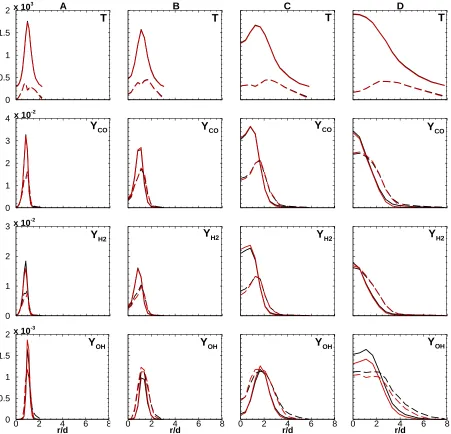
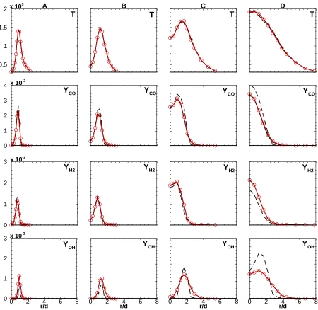
Figure 4.9. Radial profile comparisons between experimental data (symbols) and closure model (Red) of temperature, mixture fraction and measured species at x/d = 15 for flame D. ... 135

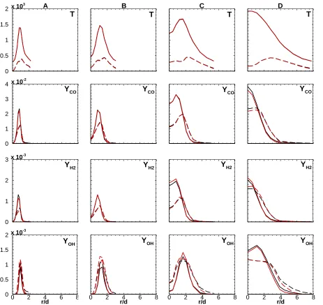
Figure 4.13. Radial profile comparisons between experimental data (symbols) and closure model (Red) of temperature, mixture fraction and measured species at x/d = 15 for flame E. ... 139

(17)

xiii Figure 4.15. Radial profile comparisons between experimental data (symbols) and closure

model (Red) of temperature, mixture fraction and measured species at x/d = 45 for flame E. ... 141 Figure 4.16. Radial profile comparisons between experimental data (symbols) and closure

model (Red) of temperature, mixture fraction and measured species at x/d = 60 for flame E. ... 142 Figure 4.17. Radial profile comparisons between experimental data (symbols) and closure

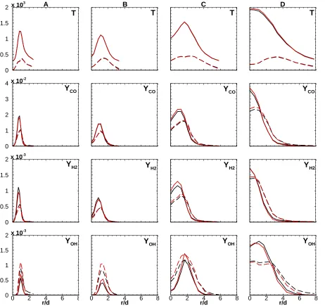
model (Red) of temperature, mixture fraction and measured species at x/d = 15 for flame F. ... 143 Figure 4.18. Radial profile comparisons between experimental data (symbols) and closure

model (Red) of temperature, mixture fraction and measured species at x/d = 60 for flame F. ... 146 Figure 4.21. Axial profile comparisons between experimental data (symbols) and closure

model (Red) of temperature, mixture fraction and measured species at the

centerline for flame D. ... 148 Figure 4.22. Axial profile comparisons between experimental data (symbols) and closure

centerline for flame E. ... 149 Figure 4.23. Axial profile comparisons between experimental data (symbols) and closure

centerline for flame F. ... 150 Figure 4.24. Flame D radial profile comparisons of experimental data (symbols) and the

closure model (Red solid lines) of the RMS of temperature and measured

(18)

xiv Figure 4.25. Flame E radial profile comparisons of experimental data (symbols) and the

species mass fractions at x/d = 15, 30, 45 and 60. ... 153 Figure 4.26. Flame F radial profile comparisons of experimental data (symbols) and the

species mass fractions at x/d = 15, 30, 45 and 60. ... 154 Figure 4.27. Radial profile comparisons between experimental data (symbols) and closure

model (Red) of temperature, mixture fraction and measured species at x/d = 1 for flame FJ200-5GP-Lr75-57. ... 159 Figure 4.28. Radial profile comparisons between experimental data (symbols) and closure

(19)

xv Figure 4.35. Radial profile comparisons between experimental data (symbols) and closure

(20)

xvi Figure 4.45. Radial profile comparisons between experimental data (symbols) and closure

model (Red) of temperature, mixture fraction and measured species at x/d = 15

for flame FJ200-5GP-Lr300-59. ... 177

Figure 4.46. Radial profile comparisons between experimental data (symbols) and closure model (Red) of temperature, mixture fraction and measured species at x/d = 20 for flame FJ200-5GP-Lr300-59. ... 178

Figure 4.47. Radial profile comparisons between experimental data (symbols) and closure model (Red) of temperature, mixture fraction and measured species at x/d = 30 for flame FJ200-5GP-Lr300-59. ... 179

Figure 5.1. Flamelet model implementation in a CFD code (Ansys Fluent 19.0). ... 183

Figure 5.2. Proposed ML modeling framework. ... 187

Figure 5.3. Training multiple scalars individually (A) vs in a single network (B). ... 188

Figure 5.4. Adaptive MLP-Clustering algorithm. ... 190

Figure 5.5. Training time needed for various network architectures using (A) MLP-SOM (light grey), (B) MLP-SOM with scalar grouping (black) and (C) MLP without SOM or scalar grouping (dark grey) on a single processor. ... 196

Figure 5.6. Interpolation time needed for various network architectures using (A) MLP-SOM (light grey), (B) MLP-MLP-SOM with scalar grouping (black) and (C) MLP without SOM or scalar grouping (dark grey). ... 198

Figure 5.7. Training time needed for various network architectures using MLP-SOM on 96 processors. ... 199

Figure 5.8. Training time needed for different number of clusters using MLP-SOM on 24 processors. ... 201

Figure 5.9. Interpolation time comparisons for thermo-chemical scalars using (A) linear interpolation and (B) MLP-SOM function. ... 205

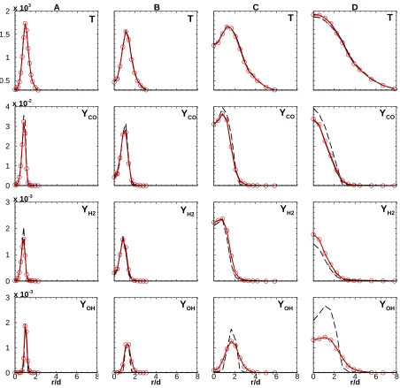
Figure 5.10. Steady-state CFD solution of Temperature for linear PDF interpolation (circle) and MLP-SOM based interpolation (solid) at x/d = 15, 30, 45, 60 and at the centerline. ... 207

(21)

xvii Figure 5.12. Steady-state CFD solution of H2O for linear PDF interpolation (circle) and

MLP-SOM based interpolation (solid) at x/d = 15, 30, 45, 60 and at the

centerline. ... 209 Figure 5.13. Steady-state CFD solution of CO for linear PDF interpolation (circle) and

centerline. ... 210 Figure 5.14. Steady-state CFD solution of OH for linear PDF interpolation (circle) and

centerline. ... 211 Figure 5.15. Steady-state CFD solution of H2 for linear PDF interpolation (circle) and

MLP-SOM based interpolation (solid) at x/d = 15, 30, 45, 60 and at the centerline. ... 212 Figure 5.16. Steady-state CFD solution of CH4 for linear PDF interpolation (circle) and

MLP-SOM based interpolation (solid) at x/d = 15, 30, 45, 60 and centerline. ... 213 Figure 5.17. Steady-state CFD solution of O for linear PDF interpolation (circle) and

MLP-SOM based interpolation (solid) at x/d = 15, 30, 45, 60 and centerline. ... 214 Figure 5.18. Steady-state CFD solution of NO for linear PDF interpolation (circle) and

MLP-SOM based interpolation (solid) at x/d = 15, 30, 45, 60 and centerline. ... 215 Figure 5.19. Steady-state CFD solution of H for linear PDF interpolation (circle) and

MLP-SOM based interpolation (solid) at x/d = 15, 30, 45, 60 and centerline. ... 216 Figure 5.20. Steady-state CFD solution of CH3 for linear PDF interpolation (circle) and

MLP-SOM based interpolation (solid) at x/d = 15, 30, 45, 60 and centerline. ... 217 Figure 5.21. Steady-state CFD solution of C2H4 for linear PDF interpolation (circle) and

MLP-SOM based interpolation (solid) at x/d = 15, 30, 45, 60 and centerline. ... 218 Figure 5.22. Steady-state CFD solution of C2H2 for linear PDF interpolation (circle) and

MLP-SOM based interpolation (solid) at x/d = 15, 30, 45, 60 and centerline. ... 219 Figure 5.23. Mean statistics of Temperature from LES solution for linear PDF interpolation

(circle) and MLP-SOM based interpolation (solid) at x/d = 15, 30, 45, 60 and centerline. ... 221 Figure 5.24. Mean statistics of CO2 from LES solution for linear PDF interpolation (circle)

and MLP-SOM based interpolation (solid) at x/d = 15, 30, 45, 60 and

(22)

xviii Figure 5.25. Mean statistics of H2O from LES solution for linear PDF interpolation (circle)

and MLP-SOM based interpolation (solid) at x/d = 15, 30, 45, 60 and

centerline. ... 223 Figure 5.26. Mean statistics of CO from LES solution for linear PDF interpolation (circle)

centerline. ... 224 Figure 5.27. Mean statistics of OH from LES solution for linear PDF interpolation (circle)

centerline. ... 225 Figure 5.28. Mean statistics of NO from LES solution for linear PDF interpolation (circle)

centerline. ... 226 Figure 5.29. RMS statistics of Temperature from LES solution for linear PDF interpolation

(circle) and MLP-SOM based interpolation (solid) at x/d = 15, 30, 45, 60 and centerline. ... 227 Figure 5.30. RMS statistics of CO2 from LES solution for linear PDF interpolation (circle)

centerline. ... 228 Figure 5.31. RMS statistics of H2O from LES solution for linear PDF interpolation (circle)

centerline. ... 229 Figure 5.32. RMS statistics of CO from LES solution for linear PDF interpolation (circle)

centerline. ... 230 Figure 5.33. RMS statistics of OH from LES solution for linear PDF interpolation (circle)

centerline. ... 231 Figure 5.34. RMS statistics of NO from LES solution for linear PDF interpolation (circle)

(23)

1

: Introduction

Combustion is a highly complex process with a strong interaction between the physical and chemical aspects of flow. The flow physics is governed by various processes including advection and dissipation of a fluid mixture, while the chemistry is governed by the production and consumption of the different components that make up that mixture. The interaction between these different processes results in the phenomenon known as combustion.

Combustion is prevalent in the 21st century and has applications in several industries including automotive, oil and gas, power generation etc. The products of these industries play a crucial role in the life of the 21st century humans, and hence an in-depth understanding of combustion is necessary.

Experiments provide a good basis for understanding, especially for flames in laboratory settings, but they prove to be less useful in industrial devices like internal combustion engines and gas turbines. The challenge with experiments is associated with complex geometries and physics, constraints with experimental measurement techniques, and the lack of resources to carry out spatially and temporally resolved quantitative measurements. With the tremendous increase in computing power in recent times, simulations for complex fluid phenomenon including combustion are predominant. Although different in nature from experiments, the challenges associated with simulations are equally demanding. Modeling the complex physics is not trivial and requires extensive understanding of the problem, which is not available in most cases.

(24)

2 complexity due to the unsteady nature of flow that results in pockets of reacting and non-reacting zones. Turbulence-chemistry interactions (TCI) exhibit a variety of unsteady and non-equilibrium effects and result in phenomena like local flame extinction, re-ignition, and multiple modes of combustion (e.g., premixed and non-premixed). Modern research in the field of combustion focuses on capturing this interaction for better understanding of the nature of turbulent flames. The inadequacy of these models in accurately capturing the various turbulent flame phenomena leaves the door open for development of new models.

Another issue with combustion modeling is the complexity of modeling the chemistry of practical fuels. Fuel chemistry is prescribed using a chemical mechanism, which includes the possible species and the reaction pathways that may exist and their associated rates. Chemical mechanisms for complex hydrocarbon fuels generally comprise of thousands of species and tens of thousands of reactions. Most of the species are minor species including intermediates and radicals and, hence, are associated with small time and length scales. A complete description of the fuel requires the model to resolve all the time and length scales accessed by the different species. This makes turbulent combustion simulations prohibitive beyond simple, 1D problems. Thus, an important challenge in turbulent combustion modeling is the construction of models that can accurately capture turbulence and chemistry effects in flames without incurring heavy computational costs resulting from the size of the chemical mechanisms.

(25)

3

1.1. Turbulence-chemistry closure in combustion modeling

The most common approaches in combustion modeling are Direct Numerical Simulation (DNS), Large Eddy Simulation (LES), and Reynolds Averaged Navier-Stokes (RANS). Although these computational approaches are similar in formulation such that they solve the 3D, unsteady Navier-Stokes (N-S) equation to resolve the flow, the main difference between them exists in the flow and thermo-chemical variables that they transport. DNS involves the transport of instantaneous variables as opposed to RANS and LES, which solve for the averaged and filtered quantities of transported variables, respectively.

(26)

4 chemical mechanism in terms of the number of species and reactions. Lu and Law (2009), in their analysis of the cost of integrating chemistry with DNS, concluded that the computational cost differs by one order of magnitude between simple and relatively more complex fuel chemistries. As a result, most DNS studies are carried out on simple and small geometries, sometimes inside a box with integral length scales of the order of 1 cm, and moreover, rely on simpler fuel chemistries. Albeit the challenges, efforts related to reducing the cost of DNS are on the lines of accelerating chemistry by developing reduced chemical mechanisms or using simpler strategies like, In Situ Tabulation (ISAT) (Pope, 1997) and adaptive mesh refinement (Day and Bell, 2000; Aspden et al., 2016) to refine the grid only within the flame structures.

(27)

5 LES formulations remain unclosed and require modeling. This issue represents the turbulence-chemistry closure problem arising in turbulent combustion modeling.

At this point, it is crucial to understand the need and importance of adequately modeling turbulence-chemistry closure. The unclosed terms in the RANS or LES formulation, especially the chemical source terms, contain key information related to physics resulting from turbulence-chemistry interactions. Hence, an inherent challenge for turbulent combustion models is to capture the different turbulence-chemistry effects adequately over a wide class of combustion problems and, moreover, to do so in a lower-dimensional basis in order to reduce the computational costs. One of the earliest models for closure was based on the fast chemistry assumption (Bilger et al., 2005). Under this assumption, it was observed that the chemical reaction rates of species in non-premixed combustors depend on both mixture fraction and scalar dissipation. Examples of such models include the eddy dissipation model (EDM) (Magnussen and Hjertager, 1977) and the eddy-breakup model (EBU) (Spalding, 1971). The recently developed closure models can be classified under three categories, state-space models including the laminar flamelet model, PDF transport models, and low-dimensional stochastic closure models. These are discussed in more detail in the next sections.

1.2. The laminar flamelet closure model

(28)

6 residence time. Thus, at higher scalar dissipation rates, the flame residence time is small enough to produce events of flame extinction (Ranganath, 2007).

In the flamelet-based closure model, local flamelets are generated by solving 1D counter-diffusion or similar flames in the mixture fraction space for different values of scalar dissipation. These are relatively simple laminar flame calculations and, hence, can accommodate complex fuels with large chemical mechanisms. The calculated flamelet libraries of thermo-chemical quantities and chemical reaction rates, parameterized against mixture fraction and scalar dissipation, can be stored for later use. A joint Probability Distribution Function (PDF) distribution of the mixture fraction and the scalar dissipation (or more conveniently the mixture fraction variance, which is commonly modeled in terms of the scalar dissipation) is used to compute mean and RMS statistics for the different thermo-chemical quantities for the corresponding mean and variance of parameterized quantities. The construction of joint PDFs is not trivial because the nature and shape of the PDF for a given combustion problem is unknown beforehand. Hence, the flamelet model and others like it use a presumed shape and, moreover, assume a statistical independence between the governing parameters (e.g. mixture fraction, scalar dissipation, and progress variable) to avoid the construction of multi-dimensional PDFs.

The laminar flamelet solutions are integrated with the joint PDFs to generate a PDF look-up closure table, which stores the mean thermo-chemical states, T, ρ and Yi parameterized against

(29)

7 mean and variance of the mixture fraction and other parameterized quantities. Linear interpolations are computationally cheap but may require a high resolution of the PDF table to achieve an acceptable accuracy. This can significantly increase the memory storage requirements and constrain the number of parameterized quantities to typically 3 or 4. Even higher dimensions may be needed to capture either transient effects or an evolving pressure, such as in reciprocating engines. The constraints on memory storage serves as an important drawback of this approach. Machine-learning (ML) algorithms have a potential of reducing the storage requirement of such tables by using mathematical functions to represent the table quantities. However, ML-based models suffer from numerous drawbacks and newer techniques that can address these issues need to be explored. One of the scopes of this work is to develop a novel machine-learning algorithm that can alleviate these issues and potentially eliminate the storage of the PDF tables.

Due to its simplicity, the flamelet model is extremely useful in relatively complex flows where the flamelet assumption applies. However, there are many instances where the pre-selection of parameters for composition space and presumption of joint PDF shapes results in a model that falls short in capturing key turbulence-chemistry interactions. These instances include the presence of non-equilibrium effects such as extinction and reignition, the presence of multiple streams for mixing or multiple modes of combustion (e.g. premixed and non-premixed), and the presence of heat losses near boundaries. Under such scenarios, other models that can accommodate high-dimensional joint PDFs of thermo-chemical scalars must be considered.

1.3. PDF transport models

(30)

8 the PDFs in the context of turbulence theory was first introduced by Lundgren (1967). In his work, Lundgren derived coupled equations for multi-point velocity distributions and compared their properties with the kinetic gas theory. In the context of reacting flow, Dopazo and O’Brien (1974a, 1974b) were the first to consider modeled equations for joint PDFs comprising of thermo-chemical variables. These equations were resolved using finite differences. Although, simpler in formulation, finite differences result in large computational overheads given the multivariate, multi-dimensional nature of the PDF in reacting flows. Pope (1981) demonstrated the Monte Carlo methods for resolving PDF equations. Monte Carlo methods are less expensive since their memory requirements are considerably smaller and scale linearly with the dimensions of the PDF. Since then, researchers have resorted to the use of stochastic Lagrangian-based Monte-Carlo frameworks (Colucci et al., 1998; Saxena and Pope, 1998; Saxena and Pope, 1999; Xu and Pope, 2000). In the Lagrangian framework, the PDF transport equation is solved by considering a finite number of notional particles that can evolve with mixing and reaction on each computational cell. However, a large number of particles may be needed to minimize statistical errors.

(31)

9 The Lagrangian-based PDF methods have been applied to a wide range of combustion problems including piloted stabilized flames (Yadav et al., 2013; Cao et al., 2007), bluff-body stabilized flames (Dally et al., 1988; Kuan and Lindstedt, 2005) and swirling bluff-body flames (Masri et al., 2000). These methods have yielded a significant improvement in accuracy over the flamelet-based methods. However, significant work needs to be carried out on improving mixing models and finding better strategies for handling multi-dimensional joint PDFs in a cost-effective manner.

1.4. Low-dimensional stochastic models

The previous sections discussed the two limits of available closure models in turbulent combustion modeling. The presumed shape PDF models are widely used because of their ease of implementation but tend to be dissipative due to the smooth nature of the PDF. This dissipation results in loss of key information related to different turbulence-chemistry phenomena. On the other hand, PDF transport models are adept in capturing these phenomena by solving a transport equation for the joint PDF. The joint PDFs can assume a variety of shapes depending on the local field of the transported thermo-chemical and hydrodynamic variables thus allowing the model to capture key turbulent flame characteristics. However, these models are computationally expensive and depend extensively on the mixing model employed. The drawbacks of these two classes of closure models, the flamelet and PDF transport models, leaves abundant opportunities to develop models that can adopt advantages of both.

(32)

(33)

11 Moreover, the numerical data generated from both LEM and ODT have been used to construct closure models for turbulent combustion that can be integrated with RANS or LES flow solvers. Ranganath and Echekki (2006, 2008, 2009) used different realizations of ODT solutions for the Sandia piloted jet flames D and F (Barlow and Frank, 2003) to construct conditional statistics, which were integrated with beta shaped PDFs to construct a closure for a RANS framework. An extension of this work was carried out recently by Miles and Echekki (2018). In their work, spatial filtering was carried out on data from different ODT realizations to construct univariate Filtered Density Functions (FDFs) for temperature and mixture fraction on each spatial filter. The FDFs were constructed using a Kernel Density Function approach (Bowman and Azzalini, 1997) and could assume arbitrary shapes ranging from a delta to a Gaussian function. The ODT-based closure was demonstrated in LES of the Sandia piloted jet flames D and F. Similar closure models have been constructed based on LEM (Goldin, 2005; Goldin and Menon, 1998, 2007; Sankaran et al., 2009; Calhoon et al., 2015). In their study, Goldin and Menon (1998, 2007) constructed joint Scalar PDFs based on LEM solutions of jet diffusion flames, which showed qualitative improvements over presumed shape PDFs in their ability to capture turbulent-chemistry interactions. The joint scalar PDFs were parameterized on a smaller set of moments. Sankaran et al. (2009) and Calhoon et al. (2015) also demonstrated the joint scalar PDF construction based on LEM data using different sets of lower-dimensional variables.

1.5. The experimental data-based closure framework

(34)

pre-12 selection of parameters for the composition space is not trivial. Several studies have explored the use of principal component analysis (PCA) to identify lower-dimensional manifolds in order to parameterize the composition space using principal components (PCs) (Ranade and Echekki, 2019; Mirgolbabaei and Echekki, 2013, 2014, 2015; Parente et al., 2011; Coussement et al., 2012). Because PCs are derived directly from data, they can potentially serve as better conditioning parameters as opposed to the traditional choices.

In turbulent combustion, multi-scalar point or line experimental measurements are the gold standard and are extensively used for validation of these various closure models. Experimental measurements contain key information related to turbulence-chemistry interactions, which can potentially be used to construct accurate closure models. However, it is unclear as to how and what information needs to be extracted and the type of experimental data that may be required. Additionally, experimental measurements may suffer from several other challenges such as the inadequacy of data, measurement uncertainty, and the absence of reaction rate information that need to be addressed before attempting to construct closure models. These issues raise questions as to the possibility of multi-scalar experimental measurements to construct closure models.

(35)

13 The idea here is to extract physics contained in experimental data and represent it in the form of mathematical models, which are computationally cheap and yet accurate in capturing the different turbulent-chemistry phenomena. The strategies proposed in this framework are novel and represent an important and new paradigm in turbulent combustion modeling. Next, a review is presented of different machine-learning models implemented for various combustion applications.

1.6. Machine-learning models in combustion

Machine-learning (ML), a subclass of artificial intelligence (AI), is set of techniques used to construct mathematical models trained on sample data, in order to make predictions and decisions for future tasks. The accuracy of future predictions depends on the accuracy and performance of the ML model during training as well as the extent, resolution, and quality of the training data. Generally, ML models have good predictive capabilities and can represent functions with very high degrees of nonlinearities as long as the data lies within the training data space.

(36)

14 because it involves segregating input data into groups or clusters based on similarity of characteristics between any input vector and other entries comprised in a certain group. A simple example of classification in the context of combustion would be grouping data from a look-up table into smaller chunks based on the values of mixture fraction and scalar dissipation rate. Because the output of a classification task is a group number represented as an integer or a character, the best way to measure the accuracy of such a task is by calculating the percentage of correct predictions. Some of the classification-based machine-learning techniques include self-organizing maps (SOM) (Kohonen, 1996), KNN (Altman, 1992), and decision trees (Quinlan, 1986).

(37)

15 temporal evolutions in combustion applications. In a follow up work, Blasco et al. (2000) clustered the composition space using SOMs and coupled it with multi-layer perceptron networks to build models over individual clusters. This technique allowed for the use of more complex chemical mechanisms. Ihme et al. (2008, 2009), Emami et al. (2012) and Owoyele et al. (2019) used ANN-based mathematical functions to replace the storage of look-up tables in the flamelet approach. Sen et al. (2010a, 2010b) and Chatzopoulos et al. (2013) applied ANNs to construct a subgrid scale closure model in LES of turbulent flames. Franke et al. (2017) used ANNs to replace a chemical mechanism, which was then used to model a jet flame using a transported PDF combustion model. Owoyele and Echekki (2017) built a reaction rate model using a PCA-ANN framework for modeling premixed turbulent flames in a 2D DNS. Ranade et al. (2019a, 2019b) developed an ANN-based framework to construct reduced chemical mechanisms for complex fuels. In this work, a shallow ANN was used to extract fuel chemistry from "noisy" shock tube measurements, followed by a deep ANN for the construction of the reduced chemical model. Lately, Convolutional Neural Networks (CNNs) have found their way in turbulent combustion modeling, providing a promising way for modeling the nonlinear sub-grid closure terms in LES (Lapeyre et al., 2019; Nikolaou et al., 2019). Also, recently, Schoepplein et al. (2018) demonstrated the use of evolutionary algorithms for LES model development in premixed turbulent flames.

(38)

16

1.7. Objectives

The objective of this research is to focus on the turbulent combustion closure aspect of combustion modeling and, moreover, to use data-based and machine-learning techniques to develop novel closure models and explore strategies to improve some aspects of the commonly used models, such as the flamelet method. The identified objectives of this research are two-fold:

(39)

17

 The second part of this research focuses on improving the laminar flamelet based closure methods. These methods are commonly used for modeling turbulent combustion closure due to their robustness and simplicity. One of the common issues with these methods is that they require storage of multi-dimensional look-up tables that are used in CFD to recover several thermo-chemical variables from a set of lower-dimensional parameters. Several machine-learning techniques have been proposed in the past (Ihme et al., 2008, 2009; Emami et al., 2012; Owoyele et al., 2019) to significantly reduce the memory storage required by the PDF tables. Although machine-learning based models can successfully reduce the memory storage requirements, there are several drawbacks to these methods in terms of higher training time, expensive CFD computation, inaccuracy in CFD solution, etc. In this work, a novel machine-learning algorithm, MLP-SOM, is developed to address these issues.

1.8. Outline

(40)

(41)

19

: Model Formulation for

Turbulent Combustion Closure

2.1. Turbulent combustion closure – a mathematical perspective

(42)

20 truly multiscale phenomenon in both time and space with a dominant interaction between turbulence mixing and chemical reaction.

Typically, the equations of instantaneous conserved quantities are expressed in a Eulerian framework. The compressible form of the non-conservative form is presented here. A more detailed version of other forms can be found in textbooks by Echekki and Mastorakos (2010), Kuo (2005), Williams (1985), and Poinsot and Veynante (2005).

Continuity transport equation:

_u ₀ t



_

  _ (2.1)

Momentum transport equation:

_, 1

N

k k j k

Du

p Y f

Dt

  



    



(2.2)

Species transport equations (k = 1, N):





k

k k k

DY

V Y Dt



  







(2.3)

Energy transport equation:

1

:

N

k k k k

De

Q p u u Y f V

Dt

  



      



(2.4)

In the above equations D Dt refers to a material derivative, ρ is mass density, u is the velocity vector, p is pressure, fk is a body force associated with kth species per unit mass, τ is the viscous

stress tensor, V_k is the diffusive velocity of kth species, _k is the kth species reaction rate, e is the mixture internal energy, which may be expressed as

1

N k _k k k

e h Y p 



(43)

21 equations that a number of terms are not explicitly represented as functions of the transport quantities and must rely on constitutive and other auxiliary relations for their definition. These relations are theoretical or empirical approximations and serve as a first level of multi-scalar treatment for turbulent combustion flows. Using the constitutive relationships, the viscous stress may be represented as follows:

   

2





I 3

T

u u u

 

 _    __

 

 _ 

 _{ } _ (2.5)

where µ is the dynamic viscosity and κ is the bulk viscosity. The species diffusive velocities are represented using the Fick’s law as shown in Eq. (2.6).

m k k k k

Y V  D Y (2.6)

Here, D_km represents the mixture averaged mass diffusion coefficient for species k. The heat flux, Q is dominated by the gradient of temperature, also known as the Dufour effect, while the chemical reaction rates for the species are derived from the law of mass action where parameters of the Arrhenius equation are obtained from a chemical mechanism. The formulation of species reaction rates or source terms is multi-dimensional, highly nonlinear, and spans a wide range of time scales from the slowest to the fastest reactions, resulting in stiff systems of equations for their solution. A detailed description of their formulation can be found in Kuo (2005). In this analysis, the following convention is adopted: the reaction rate and source terms of species are proportional and are only different by the factor of density. Hence, these terms may be used interchangeably in the remaining chapters.

(44)

22 chemistry interactions. DNS is a class of techniques that resolve these instantaneous conservation equations across all scales for turbulence and chemistry and obtain accurate representations of reacting turbulent flow structures. The spatial-resolution requirement scales to around the cube of the Reynolds number, while the time-resolution requirement scales with the time scales of the fastest species in the chemical system (Prosperetti and Tryggvason, 2009). The diffusive and reactive nature of intermediate species also affects the spatial scales, especially near the flame front. This mixed nature results in very fine mesh sizes and extremely small time steps, thus constraining DNS to modeling problems at smaller Reynolds numbers with simpler chemical systems over uncomplicated geometries.

(45)

23 accurate than RANS due to its inherent ability to capture the interaction between mixing and chemical reaction for large-scale flow structures. Moreover, LES can be easily combined with other low-dimensional stochastic models such as ODT and LEM, which can be designed to capture subgrid-scale physics. More importantly, both averaging and filtering of instantaneous conserved quantities result in unresolved physics over a range of time and length scales. In RANS, the unresolved physics exists over an entire range of time and length scales accessed in a given problem while in the case of LES, the ‘missing’ physics rests only in the smaller or subgrid scales. Nonetheless, these missing scales and the related physics associated with them need to be modeled in order to accurately predict the interaction of physics and chemistry existing in a flow.

Mathematically, the averaged or filtered conservation equations contain quantities that cannot be explicitly represented with the existing transport variables. For a more detailed understanding of these unclosed terms, a typical RANS/LES formulation of the instantaneous conservation equations is as follows:

Averaged/filtered continuity transport equation:

_u ₀ t



_

  

 (2.7)

Averaged/filtered momentum transport equation:

_,





1

N

k k j k

Du

p Y f u u

Dt

   



 

    



  (2.8)

Averaged/filtered species transport equations (k = 1, N):







' '



k

k k k k

DY

V Y u Y

Dt

          (2.9)

(46)

24

1

: ( )

N

k k k k

De

Q p u u Y f V u e

Dt

   



 

      



 (2.10)

In the above equations, the symbols “̅“and “̃” correspond to Reynolds averaging and density weighted averaging, respectively, where is the mean or filtered density, 𝑢̃ is the velocity, Y_k is the species mass fraction, and 𝑒̃ is the internal energy. The averaged or filtered reaction rate term in the species transport equation and the advection terms in all the equations are highly nonlinear and remain unclosed because explicit relationships to compute them in terms of transport quantities are not trivial. On the other hand, models for some of these terms are well established. The Reynolds stress tensor,

 

u u  in the momentum transport equation, is popularly modeled using the Boussinesq approximation:

2 3 t

u u



u q



     (2.11)

where 𝑞̃ is the turbulent kinetic energy, _tis turbulent viscosity, and  is a Kronecker delta function. In this approximation, the unclosed Reynolds stress tensor is expressed in the form of the averaged/filtered velocity gradient and another constant called the turbulent viscosity (Wilcox, 1998). This turbulent viscosity is in turn modeled using different turbulence models, including k -ε (Shih et al., 1995; Smagorinsky-Lilly (Smagorinsky, 1963), etc.), depending on whether a RANS or LES formulation is used. The spatial filter is generally included in the turbulent viscosity for LES formulations. The scalar fluxes in the species transport and energy equations have a similar approximation called the gradient diffusion approximation, which results in a turbulent diffusivity

t

(47)

25

t t

D Sc



 (2.12)

where Sc is the Schmidt number.

The models for Reynolds stress and scalar flux are relatively well established, however, the most critical requirement of closure arises from the modeling of the mean or filtered reaction rate term. The reaction rate is a highly complex term with nonlinear contributions from multiple species and temperature. In DNS, the computation of reaction rate is straightforward because the mathematical formulations and related parameters are readily available in a chemical mechanism. The difficulty arises when the averaged or filtered values of these nonlinear quantities need to be determined in the cases of RANS and LES. In general, the mean of any nonlinear function is not equal to the nonlinear function computed from the means of the dependent variables. In the context of the reaction rate, Eq. (2.13) describes this inequality,





( , ,

T Y Y

1 2

,...,

Y

N

)









T Y Y

, , ,...,

1 2 YN



(2.13)

The issue of turbulent combustion closure exists because of this inequality. The significant difference that exists between the two quantities prevents the use of chemical mechanisms for modeling combustion chemistry within the context of RANS and LES. Since a direct mathematical formulation is not available, the averaged or filtered reaction rates need to be modeled by other means. These reaction rates carry information from all the missing scales and can be representative of several different turbulent flame phenomena.

(48)

26 method for turbulent combustion closure, namely the laminar flamelet method. In the following sections, the mathematical formulation of the laminar flamelet approach as well as the experimental data-based closure framework are discussed.

2.2. The laminar flamelet model

In the laminar flamelet method (Peters, 1983, 1984), the averaged or filtered thermo-chemical space including temperature, density, specific heat, mixture properties and mass fractions of species are represented in a lower-dimensional manifold using a set of pre-defined conditional parameters. From turbulence theory, the average of any quantity can be calculated by integrating the conditional mean of that quantity convolved with a joint probability density function (PDF). Mathematically, the averaged or filtered thermo-chemical variables within the context of the flamelet model are represented in Eq. (2.14), as follows:

2

|

; , ''

k

P



d



 

_

 

_



 



_

(2.14)

where







T, , ,



Y Y₁ ₂,...,Y_n



and the lower dimensional parameters,





 

Z,



for an adiabatic steady diffusion flamelet model. Z and



are traditional choices of parameters and represent mixture fraction and scalar dissipation respectively.

It is evident from Eq. (2.14) that there are two components to this model, 1) the conditional means, which are specific to the composition space accessed by the problem, and 2) the joint PDFs that store information on the turbulence-modulated statistical distribution of the thermo-chemical scalar values. In the flamelet model, the conditional mean statistics are based on 1D laminar flame solutions modeled in their simplest forms by a quasi-1D counter-flow configuration in the Z and

(49)

27 formulated in the mixture fraction, Z,and scalar dissipation,



, space. The mathematical formulation of the so-called flamelet equations is given below for species and temperature:

2 2 . 2 i i i Y Y t Z     

 _ (2.15)

2

1

2 2

pi _i pi

i i

i p

i i

C _Y C

T T T p

h

t _Z Le Z Z Z C t

 

_      _ _ _  __   _

 



  



 (2.16)

The scalar dissipation,



represents the contribution of molecular diffusion in mixture fraction space. Equations (2.15) and (2.16) are solved for different values of the scalar dissipation to construct conditional mean statistics in the mixture fraction and scalar dissipation space.

The flamelet approach uses a presumed shape beta PDF in the Z space and a delta PDF in the



space. A statistical independence is assumed to express the joint PDFs as a product of the univariates of the two parameters. A typical beta PDF in the mixture fraction space can be represented as shown in Eq. (2.17):





1 1 ₁ ( ) ( ) ( ) ( ) Z Z P Z         _   

  (2.17)

where  is gamma function,





Z



,



 

(1

Z

)



, and

 

2 1 '' Z Z Z



  .

The coefficients  and  are related to mean and variance of mixture fractions allowing for construction of different PDFs by simply changing these quantities. In the flamelet approach, the conditional statistics are integrated over different beta and delta PDFs to construct a three-dimensional look-up table such that:

2

( , '' , )

f Z Z

(50)

28 In general, a look-up table may easily contain more than three dimensions depending on the number of parameters retained for constructing the lower-dimensional manifold. For example, a look-up table generated from a non-adiabatic steady diffusion flamelets also contains total enthalpy as a parameterized quantity. The issue with massive multi-dimensional look-up tables is that they need to be stored in memory so as to be able to retrieve the mean thermo-chemical quantities on-demand in a CFD simulation. Some of the thermo-chemical properties, such as density, temperature, mixture specific heats, mixture molecular weight etc., need to be interpolated from the tables multiple times in every iteration of the fluid flow solver and on every cell of the computational domain. Because these tables are constructed over a broader range of thermo-chemical conditions, they tend to have several million points storing about 20-30 thermo-thermo-chemical quantities. This results into a storage requirement of gigabytes or even terabytes, as higher dimensions for the tables are needed.

(51)

29 In Chapter 5 of this work, the challenges associated with machine-learning models in the context of flamelet based turbulent combustion closure are addressed. A new machine-learning algorithm is developed and validated over several a priori and a posteriori tests.

2.3. The experimental data-based closure framework

Flamelet models, although very popular, robust and computationally efficient, are not known for their ability to accurately capture physics resulting from complex turbulence-chemistry interactions, such as the extinction-reignition phenomenon. This deficiency in these models is caused by a variety of factors. First, these models are constructed from laminar flame solutions that may or may not capture relevant physics. Hence, the thermo-chemical states accessed by the conditional mean statistics (or flamelets) may not contain information of different turbulent combustion phenomena. Second, flamelet models rely on presumed shaped beta PDFs, which tend to be dissipative and may not capture the true nature of turbulence occurring in a given flame. Beta PDFs are not designed to be bimodal and, hence, are inadequate in capturing effects such as local flame extinction, reignition. Such events are known to be associated with bimodal-shaped PDFs. Barlow and Frank (2003) demonstrated the association of bimodal behavior with local extinction in their series of experiments over the Sandia piloted jet flames D, E and F. Finally, the flamelet model relies on traditional choices for parameterized variables. However, in many instances the choice of parameterized variables is not trivial. The traditional choices may not be adequate to capture the necessary physics.

(52)

30 flame, they may potentially be very useful in the construction of a closure model. The Turbulent Nonpremixed Flames (TNF) Workshop (https://www.sandia.gov/TNF/abstract.html) provides a resource for such measurements over broad thermo-chemical or hydrodynamic conditions for a variety of flames. Some of the flames included in this database are pilot-stabilized jet flames with and without inhomogeneous inlets, bluff-body stabilized flames, swirl flames etc. While the flames measured for the TNF Workshop have been primarily the testing beds for turbulent combustion closure models, it is easy to perceive the potential of such measurements in practical flows where a simple description of the statistics can no longer be represented in terms of the usual set of prescribed parameters. However, there are several questions that need to be answered to enable the construction of such a framework.

(53)

31 PCA proves to be an optimal tool in parameterizing the composition space, ICA has also been explored in a similar context.

(54)

32 In general, experimental databases of turbulent flames contains information of temperature and mass fractions of major species whose concentrations are large enough to be adequately captured barring interferences between the optical signals. However, there is no information available related to source terms of these thermo-chemical quantities. Additionally, information related to smaller intermediate species (such as H, O, CH3) is not always readily available. These intermediates are integral components of the chemical source term computation of temperature and other measured species. The unavailability of such source terms or reaction rates or intermediate species precludes the construction of a closure model that can be based on experimental data.

In this work, a novel methodology is proposed, which uses a modified version of pairwise mixing stirred reactor (PMSR) (Pope, 1997; Yang and Pope, 1998) to approximate the source terms of measured temperature and reaction rates of measured species for each and every instantaneous measurement. The idea behind PMSR is to allow local mixing and reaction of different instantaneous measurements to allow the evolution of all the unmeasured intermediate species in a given chemical mechanism. This choice, in turn, allows construction of conditional means for the chemical source terms, which can be integrated over joint PDFs at each spatial location in a PC space to recover the mean or filtered source terms and reaction rates of temperature and measured species, respectively. Subsequently, the PC source terms can be determined using the relations described in the discussions below.