Dynamic Modelling for the Assessment Of Seismic Fragility of NPP Components
Giorgio Bianchi, Davide Carlo Mantegazza, Federico PerottiDepartment of Structural Engineering, Politecnico di Milano, Italy
ABSTRACT
The criteria for developing structural models of a NPP reactor building are discussed; attention is mainly focused on models which are suitable for verifying the seismic performance of components, either by the Floor Response Spectrum approach or by direct analysis.
The finite-element approach is here considered as an alternative to more traditional stick models and is applied to an illustrative example. For this two models have been set; the first one, more refined, is suitable for the assessment of both stuctural and equipment components. The second model is a simplified one, intended for computing in-building response for equipment design; validation is performed by comparing modal properties of the two models.
Within the context of simplified FE modelling, the adoption of consolidated criteria for representing complex interaction phenomena has been also addressed. This is the case of soil-structure interaction and fluid-structure interaction due to the sloshing effect in the RWST pools; in both cases lumped-parameter simplified models are available for the rigid foundation and rigid reservoir hypotheses. Criteria for coupling these models with FE discretizations are here discussed and applied.
INTRODUCTION
This paper summarizes, with reference to an illustrative example, criteria and hypotheses adopted in developing structural models for studying the seismic response of a NPP reactor building. Seismic analysis is here intended to fulfil the following needs.
1. Support the equipment designers with seismic actions at specified locations in the building. 2. Support “conceptual” structural choices during the preliminary design of the building.
3. Compute extreme values of response under design seismic actions for checking the resistance of the structural elements of the building.
4. Compute the actual risk associated to building or equipment failures under seismic actions.
With reference with the first of the quoted tasks, it is here assumed that for normal equipments a two stage analysis can be performed to evaluate seismic demand. In the first phase a complete model of the building is set, where equipments are taken into account as distributed or lumped masses which are rigidly connected to the structural elements; in the second phase the dynamic analysis of the equipment is performed assuming as seismic input the building response at its supports. Within this context it is deemed that, given the structural properties of normal reactor buildings, a reasonably simple linear elastic model can be used for the first analysis. The level of refinement of the equipment modelling, on the other hand, will depend on its importance and anticipated fragility.
In the second task basic design choices are addressed, such as the foundation typology, the introduction of an isolation system, the general structural layout, the roofing system, etc.; to this purpose, a simplified model of the building seems to be suitable as well for performing repeated dynamic analyses.
A more refined model is needed, on the contrary, to compute design seismic effects (stresses or internal forces) in the building structural elements; this model can be efficiently developed in parallel to the simplified one, in order to validate it in terms of overall structural response.
Similar considerations hold when the performance of fragility analysis of equipment components [1] is considered as a step of seismic risk assessment (point 4). Note that this type of analysis requires, regardless of the technique adopted, the performance of a large number of structural response evaluations, which are necessary to estimate the influence, on building and equipment response, of a number of randomly variable parameters. The use of simplified building models is thus mandatory for practical reasons.
It can be anticipated, on the other hand, that fragility of building structural components will hardly dominate the seismic risk; assuming that problems can be confined into a small number of elements, local refinement can be sought within overall simplified models.
Finally, if the resistance of the foundation ground appears to critical in terms of seismic fragility, the problem seems again tractable upon use of simplified building models resting on more refined ground discretizations.
As a result, the problem of developing and validating simplified models of NPP reactor buildings seems to be worth a research effort; particular attention will be here devoted to the use of finite element models, as an alternative to more traditional “stick models”.
are valid for the scope here pursued, which is the validation of the simplified approach by means of comparison between the results obtained with the two models.
REFINED MODEL OF THE REACTOR BUILDING
In light of the preceding consideration, a refined model (called model A), encompassing a degree-of-freedom number of the order of 106, was preliminarily set. Modelling was restricted to the structural system, which was assumed as fixed at the foundation mat base; this is justified by the fact the model was here used only for validating the criteria for simplified discretization of the building, while validation of soil models was beyond the scope of the performed activity.
In a real application, in which soil data will be available for the specific site and where the model will be use for a complete structural safety evaluation, it is intended that the refined building model is to be completed by a 3D finite-element soil mesh, taking account of soil properties variation and other local conditions.
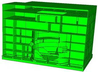
The main structural elements of the building (see figure 1) have been introduced according to the criteria summarized in the following. Reference is made to the elements and modelling options available in the ABAQUS structural analysis code [2].
Foundation mat 8 node solid elements have been placed in 3 layers. Approximate element size is 0.65 m. Total thickness is 2 m.
Structural walls All walls directly supported by the foundation mat have been introduced, by means of 8 node shell elements. Element size is about 1 m, while thickness is 1 m.
Shielding wall It is a cylindrical wall having a thickness of 1.5 m and surrounding the containment system. Has been modeled via shell elements, with approximate size of 1 m.
Slabs A thickness of 1 m has been assumed for all structural slabs. Shell elements have been used; size is approx 1 m. Roofing system A flat slab with stiffening girders was assumed; the slab was modelled via shell elements (1 m thickness). Girders were introduced with a 5 m spacing and a total depth of 3 m. They were represented by 3D beam elements; at each node, the element centroid is connected to the corresponding shell node with a rigid link.
All the shell elements introduced in the model are of the so called “general purpose” type, which is suitable for modelling both thick and thin shell systems. The connection between shell and solid elements have been treated via the SSC (Shell-to-Solid Connection) option. This imposes locally to the solid surface the shell kinematic assumption (segments orthogonal to the mean surface remain straight); shell internal forces are transmitted to the solid mesh nodes according to weighted tributary areas, in order to reproduce membrane and flexural stress distributions.
Fig. 1 Structural elements of the reactor building
In addition, all the quoted structural elements share the same material model; reinforced concrete is assumed to behave as a linear elastic, homogeneous and isotropic medium, having a Young modulus of 35000 MPa, a Poisson ratio of 0.17 and a density of 2500 kg/m3.
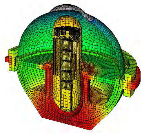
Containment A 44.5 mm thick steel sphere is assumed, modelled by means of shell elements. The latter have an approximate size of 0.2 m. Steel is modelled as an elastic material as well, having a Young modulus of 200000 MPa, a Poisson ratio of 0.3 and a density of 7850 kg/m3. The lowest half of the sphere is supported (see figure 2) by a massive reinforced concrete structure; this is modelled by means of 8 node brick elements. At the interface with the vessel shell, 20 node elements have been introduced. Perfect bond is assumed between steel and concrete at both sides (internal and external) of the shell.
Fig. 2 Containment and supporting structure
Vessel and internals The pressure vessel structure (figures 2-3) is made by a cylindrical shell having a diameter of 6.5 m, closed by two hemispherical heads. Total height is 22.15 m, while thickness is 144 mm, 280 mm and 203 mm for the upper head, the shell and the lower head respectively. Supporting plates have been modelled as rigid bodies.
The vessel external shell is connected to lower part of the containment by a means of a 120 mm frustum-shaped plate. Shell elements have been used for its modelling (figure 5).
The vessel internals have been represented by preserving, as much as possible, the actual geometry and inertia; components have been modelled as rigid, or highly stiff, bodies, by using solid elements and constraint options. These rigid bodies have been connected to the vessel shell by means of distributed (DCC) connections, in order to reduce spurious stiffening.
Taking temperature effects into account, a Young modulus of 180000 MPa has been assumed for structural steel of the vessel elements.
The water contained in the vessel has been treated as a rigid body, which is attached to the shell via a distributed connection (DCC), equally subdividing the inertia forces developing in the water between the selected nodes on the vessel shell.
Sloshing effect in the suppression pools The suppression pools which are located within the containment have been modelled as rigid bodies, connected to the r.c. structure by means of a DCC connection.
The structure of the RWST pools has been modelled by means of shell elements. For modelling the water content taking account, though in a simplified way, of the sloshing effect it has been assumed that the r.c. structure can be regarded as rigid in terms of interaction with the fluid. In this light, the classical simplified solution for the sloshing effect in rigid rectangular tanks have considered; the solution accounts for the first sloshing mode in one direction, by splitting the liquid mass into an “impulsive” mass m0 (at a height h0), constrained to the tank walls and a “convective” lumped
mass m1 (at a height h1), free to move horizontally and connected to the tank by means of a horizontal spring of stiffness
k1. Different values of the constants are assigned for sloshing in the two horizontal directions. For each direction, the
impulsive mass is here distributed throughout the tank walls, with a center of gravity at height h0. The convective mass is
assigned to a rigid body, having the center of gravity at a height h1; the body, which is only free to translate in the
horizontal plane, is connected to the nodes of the tank walls model through a double distribution of springs (one set for each direction), each having a total stiffness equal to k1 (k1xor k1y according to the direction) and acting in normal
direction with respect to the wall plane.
Fig. 3 Refined finite element model of the vessel
SIMPLIFIED MODEL OF THE REACTOR BUILDING
The simplified model (model B) have been obtained by applying the following criteria. Walls, slabs and foundation mat Have been modelled by means of shell finite elements. Roof The same discretization as in the refined model has been adopted.
Containment The lower part of the containment, encompassing the lower steel hemisphere and the surrounding reinforced concrete supporting structure have been modelled as a rigid body.
The upper part of the sphere has been represented via an equivalent 2-dof inverted pendulum system (figure 4). This is defined by three fixed parameters, i.e. the bar lengths l l1,2 and the ratio χ=I1
/
I2 between the bar moments of inertia and by five variables, m m k k1, 2, 1, 2 and I= +I1 I2. These are obtained by imposing the equivalence between the model and the hemisphere, in terms of the following parameters: center of gravity position, total mass, moment of inertia and natural frequencies of the two fundamental vibration modes.The model has been validated for the values l1= =l2 5.45 ,m I2 =0 by comparing its response to the one of the hemisphere under a prescribed base acceleration history. The comparison has been performed in terms of acceleration time histories at two different levels and of base shear, showing satisfactory results.
Vessel Simplified modelling has been suggested by the observation of the lower vibration modes of the refined model, where elastic deformation is confined to a rather limited zone centered on the supporting plate. On this basis the lower and upper part of the vessel shell have considered rigid (see figure 8) while the central portion of the shell have been discretized via shell elements; the elastic modulus of these elements has been slightly adjusted for a better match of the natural frequencies of the two vessel models (refined and simplified).
refined model has been maintained. Again, the model has been satisfactorily verified in terms of response to a base acceleration time history.
1
I
2
I
2
m
1
m
2 q
1
q
2
k
1
k
1
l
2
l
Fig. 4 Simplified models for containment (left) and vessel (right)
Foundation ground model In using a simplified 3D finite element models for the building structure a question arises whether a similar model must be adopted for the foundation medium as well. When, in addition, a preliminary design phase is considered in which the properties of the ground are still largely hypothetical, the resulting computational effort seems to be hardly justified. On the other hand, simplified solutions based on the use of available impedance functions are restricted to the case of rigid foundations. To overcome this difficulty and to exploit the structural properties of the reactor building, it has been here assumed that the foundation mat, when stiffened by all structural walls, can be treated as “quasi-rigid”. This means that its deformability is taken into account in modelling it as a part of the structural system, but that it can be neglected with respect to soil-structure interaction effects.
On practical grounds this criterion leads to the following modelling procedure.
• Soil impedance functions are first computed (see [3]), in terms of lumped elastic and viscous elements properties, for the rigid foundation case. To this purpose a tangential modulus Gs=200 MPa and a Poisson ratio
s
ν =0.33 have been considered for soil, along with a foundation “effective” embedment of 10 m.
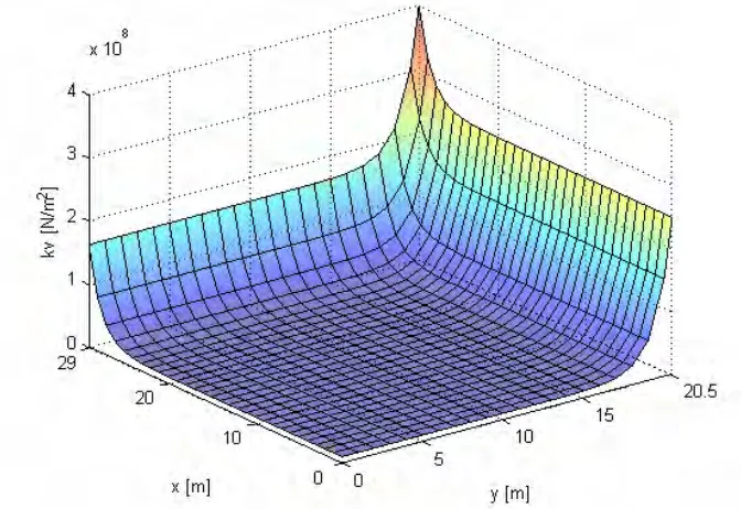
• A distributed layer of spring and dashpots is placed at the nodes of the foundation model, matching the total stiffness and damping values for the six rigid body motion components. In doing this advantage is taken from shell modelling of the mat, which allows for the introduction of rotational distributed springs. The latter can be necessary to reach the correct value of rocking stiffness, though maintaining a reasonable distribution to the stiffness of vertical spring.
As an example, in figure 5 the distribution obtained for the vertical stiffness of the local springs is illustrated for one fourth of the mat foundation. The simplified model taken soil-structure interaction into account is called B1 in the following.
MODAL ANALYSIS OF THE REFINED AND SIMPLIFIED MODELS
In Table 1 the natural frequencies of the most significant vibration modes are compared for the two models in the rigid foundation case (models A and B). The modes considered in the table are two cantilever modes, in each direction, a vertical and a torsional mode for the building, two rocking modes and one vertical mode for the vessel and two horizontal translation modes for the containment.
Table 1. Natural frequencies of the lowest vibration modes of models A and B
Mode Refined (A) [Hz]
Simplified (B)
[Hz]
∆
[%] Mode description
11 5.41 5.60 +3.5 1 “cantilever” mode in y direction
12 6.42 6.66 +3.7 1 “cantilever” mode in x direction
15 8.22 8.54 +3.7 Torsional mode
21 12.31 12.70 +3.2 2 “cantilever” mode in y direction
31 15.56 16.4 +5.4 2 “cantilever” mode in x direction
24 13.55 13.52 -0.2 1 vessel rocking mode y-z plane
25 13.56 13.52 -0.2 1 vessel rocking mode x-z plane
92 31.38 30.79 -1.88 vessel mode translation in z direction
90 30.56 30.43 -0.42 1 containment mode y direction
91 31.12 31.06 -0.19 1 containment mode x direction
22 13.06 13.42 +2.75 1 global mode vertical translation
34 16.58 17.01 +2.6 2 global mode vertical translation
As it can be noted, natural frequencies of the two models compare satisfactory for all types of normal modes. In Table 2 the results of the modal analysis of model B1, i.e. when soil-structure interaction is considered, are summarized. Natural frequencies of lower modes are given together with a brief description of the modal shape. The lower modes not appearing in the table are relative to water sloshing or to local vertical motion of the roof.
It can be noted how lower modes of the soil-interacting model are at frequencies (between 2 and 2.5 Hz) where horizontal earthquake excitation exhibits its largest harmonic components. Vessel local modes, on the other hand, show natural frequencies between 10 and 20 Hz, where more limited spectral amplifications can be anticipated.
Comparing the results in tables 1 and 2 it can be also inferred how soil-structure interaction, even though firm ground conditions have been assumed, heavily affects the first global modes. On the contrary, very little influence on local vessel modes is detected.
In figures 6 and 7 some examples of modal shapes are given. In the first a global rocking mode is represented, while in the second rotation of the vessel simplified model occur, resulting in deformation of the central part of the vessel (shell FE discretization - in black) and rotation of the upper and lower rigid bodies (red lines in figure 4 becoming blue lines in figure 7).
Table 2. Natural frequencies of the lowest vibration modes of B1 model
Mode
Natural frequency
[Hz]
Mode description
5 2.084 global z translation
6 2.161 global rocking about x axis
7 2.241 global rocking about y axis
8 3.368 global rotation about z
10 4.679 foundation rocking about x axis + y translation – “cantilever” building deformation
11 5.155 foundation rocking about y axis + x translation – “cantilever” building deformation.
18 12.128 2° “cantilever” building mode in y direction
48 18.669 2° “cantilever” building mode in x direction
19 13.177 vessel rotation about y axis
22 13.188 vessel rotation about x axis
42 18.669 vessel x translation
43 18.813 vessel y translation
94 30.237 vessel z translation
Fig. 6 Example of rocking mode of the simplified model
Fig. 7 Example of vessel mode (simplified model)
CONCLUSIONS
The development of finite element models for the dynamic analysis of NPP buildings has been addressed, with particular attention to simplified models allowing for the performance of a large number of simulations at a reasonable computational cost.
Two models have been set for an illustrative example regarding the preliminary layout the of a reactor building; one is a refined model, here used for validating, in terms of modal properties, a more simplified FE discretization. Within the development of the second model two problems have deserved particular care; the first one is the simplified representation of soil-structure effects. A solution is proposed based on the hypothesis (quasi-rigidity) that the foundation mat, though represented by an elastic FE discretization, can be still treated as rigid with respect to the soil medium; on this basis a criterion is formulated for taking soil stiffness and damping into account without going through a costly 3D FE model.
A similar approach has been used for simplified representation of the sloshing effect in RWST pools; here the quasi-rigidity hypothesis is applied to the pool walls which, though being part of the shell discretization of the building, can be regarded as rigid in terms of fluid-structure interaction; the hypothesis allows for the use of classical “spring and mass“ sloshing models.
The problem of setting and calibrating simplified equivalent models of the containment and of the reactor vessel has been also addressed and different procedures have been developed and validated for the two components.
As a result, the comparison between the modal properties has been illustrated for the fixed base models, showing excellent agreement for all most significant normal modes.
Finally the modal properties of the complete simplified model, encompassing soil-structure interaction, have been given, showing the typical features of the dynamic behaviour of NPP buildings.
REFERENCES
[1] De Grandis, S. and Perotti, F. “An innovative methodology for computing fragility curves of NPP components under random seismic excitation”, Proceedings of SmiRT 19, Toronto, Canada, August 12-17, 2007.
[2] ABAQUS, User’s and Theory Manuals, Release 6.5, Hibbit, Karlsson & Sorensen Inc., 2004.