Mean Shift Segmentation on RGB and HSV
Image
Poonam Chauhan, R.v. Shahabade
Department of Information Technology, Terna College of Engineering, Nerul Navi Mumbai, India
Professor, Department of Electronic and telecommunication, Terna College of Engineering, Nerul Navi Mumbai, India
ABSTRACT
:
This paper compare the method of color image mean shift segmentation considering both global information and local homogeneity on HSV image and mean shift segmentation on RGB image . The method applies the mean shift algorithm in the hue and intensity subspace of HSV. The cyclic property of the hue component is also considered in the hsv image segmentation method. Experiments on natural color images show promising results.KEYWORDS: HSV color image, RGB, Mean shift , segmentation
I. INTRODUCTION
One major task of pattern recognition, image processing, and related areas: is to segment image into homogenous regions. Image segmentation is the first step towards image understanding and image analysis. Clustering techniques identify homogeneous clusters of points in the feature space (such as RGB color space, HSV color space, etc.) and then label each cluster as a different region. The homogeneity criterion is usually that of color similarity, i.e., the distance from one cluster to another cluster in the color feature space should be smaller than a threshold. The disadvantage of this method is that it does not consider local information between neighboring , pixels. In this paper, we propose a segmentation method introducing local homogeneity into a mean shift algorithm: using both global and local information. The method is performed in "Hue-Value" two-dimensional subspace of Hue-Saturation-Value space.. The proposed method considers the cyclic property of the hue component, does not need priori knowledge about the number of cluster, and it detects the clusters unsupervised. The paper is organized as follows: in section 2, ; the mean shift algorithm is introduced in section 3. The proposed color image segmentation method is given in section 3. Section 4 includes experiments on color image (real) segmentation. The conclusion can be found in section 5.
II. RELATED WORK
Image segmentation has been acknowledged to be one of the most difficult tasks in computer vision and image processing [3, 8].Unlike other vision tasks such as parametric model estimation [20, 22], fundamental matrix estimation [18], optical flow calculation [21], etc., there is no widely accepted model or analytical solution for image segmentation. There probably is no “one true” segmentation acceptable to all different people and under different psychophysical conditions. A lot of image segmentation methods have been proposed: roughly speaking, these methods can be classified into [3]: (1) Histogram thresholding [13]; (2) Clustering [6, 23, 2]; (3) Region growing [1]; (4) Edge-based [14]; (5) Physicalmodel- Edge-based [12]; (6) Fuzzy approaches [15]; and (7) Neural network methods [11]. Clustering techniques identify homogeneous clusters of points in the feature space (such as RGB color space, HSV color space, etc.) and then label each cluster as a different region. The homogeneity criterion is usually that of color similarity, i.e., the distance from one cluster to another cluster in the color feature space should be smaller than a threshold. The disadvantage of this method is that it does not consider local information between neighboring pixels.
III. THE MEAN SHIFT ALGORITHM
maximum increase in the density. The converged centre (or windows) correspond to modes (or centers of the regions of high concentration) of data. The mean shift algorithm is based on kernel
density estimation.
IV. MEAN SHIFT ALGORITHM AND KERNEL DENSITY ESTIMATION.
Let {Xi}i=1,…,n be a set of n data points in a d-dimensional Euclidean space Rd, the multivariate kernel density estimator with kernel K and window radius (band-width) h is defined as follows [1], :
ƒ̂(x)=
1𝑛𝑑
K(
x−xi h 𝑛
𝑛=1
)
(1)
The kernel function K(x) should satisfy some conditions .The Gaussian kernel is one optimum kernel, which yields
minimum mean integrated square error (MISE):
In Mean Shift we are only interested in a special case of radially symmetric kernels satisfying: K(x)=ck,
dk(∥x∥2) where ck, d, the normalization constant, makes K(x) integrate to one and k(x) is called the profile of the kernel.
It helps us simplify the calculation in the case of multivariate data.
The profile of the Gaussian kernel is: 𝑒−12𝑥^2and therefore, the multivariate Gaussian kernel with the standard
deviation \σ will be:
K(x) =1 1 2𝜋√𝜎𝑑𝑒𝑒
1 2− | 𝑥 |^2
2𝜎 ^2 (2)
Where d is the number of dimensions. It's also worth mentioning that the standard deviation for the Gaussian kernel
works as the bandwidth parameter, h.
Now having sample points {xi}i=1..n, each mean shift procedure starts from a sample point yj=xj and update yj until
convergence as follows:
𝑦𝑖0= 𝑥𝑖 (3)
𝑦𝑖𝑡+1=
𝑒−|𝑦 𝑗−𝑥𝑗 𝑡 |^2
^2 𝑛
𝑖=1 𝑒−|𝑦 𝑗−𝑥𝑗
𝑡 |^2 ^2 𝑛
𝑖=1
(4)
So basically all the points are considered in calculation of the mean shift but there is a weight assigned to each point that decays exponentially as the distance from the current mean increases and the value of σ determines how fast the decay is.
The mean shift is an unsupervised nonparametric estimator of density gradient and the mean shift vector is the difference between the local mean and the center of the window.
The mean shift vector M(x) is defined as: From equation (3) and equation (4), we get:
Mx=
^2∇̂𝑓(𝑥)𝑑+2 𝑓 (𝑥)
(5)
V. THE PROCEDURE OF THE MEAN SHIFT ON RGB AND HSV IMAGE
The Mean Shift algorithm can be described as follows: 1. Choose the radius of the search window
2. Initialize the location of the window xk, k=1. 3. Compute the mean shift vector Mh,k(xk).
4. Translate the search window by computing xk+1= Mh,k(xk)+ xk, k=k+1. 5. Step 3 and step 4 are repeated until convergence.
The mean shift automatically finds the local maximum density. This property holds even in high dimensional feature spaces. In [4], the authors also proposed a peak-finding algorithm. Unfortunately, it is heuristically based. In contrast, the mean shift algorithm has a solid theoretical foundation. The proof of the convergence of the mean shift algorithm can be found in [7, 8].
3.3. The cyclic property of the hue component in the mean shift algorithm on HSV image
Because the hue is a value of angle, the cyclic property of the hue must be considered. The revised mean shift algorithm can be written as:
M’(x)=1
𝑛𝑥′ 𝑋(𝑖)∈𝑆 (𝑥)𝑋𝑖 − 𝑥 (6)
where the converging window center x is a vector of [H, I], and 'x
n
is the number of data points inside the . . When translating the search window, let xk+1=[Hk+1,Vk+1].We have:
𝐻𝑘 +1 = 1
𝑛𝑥′ 𝑋 𝑖 ∈𝑆 𝑥 𝐻𝑖 𝑖𝑓 0 ≤ 1
𝑛𝑥′ 𝑋 𝑖 ∈𝑆 𝑘 𝐻𝑖 ≤ 255 1
𝑛𝑥′ 𝐻𝑖 + 255, 𝑖𝑓
1
𝑛𝑥′ 𝑋 𝑖 ∈𝑆 𝑘 𝐻𝑖 < 0 𝑋 𝑖 ∈𝑆 𝑥
1
𝑛𝑥′ 𝐻𝑖 − 255, 𝑖𝑓
1
𝑛𝑥′ 𝑋 𝑖 ∈𝑆 𝑘 𝐻𝑖 > 255 𝑋 𝑖 ∈𝑆 𝑥
(7)
and
𝑉𝑘+1=
1
𝑛𝑥′ 𝑋(𝑖)∈𝑆𝑣(𝑘)𝑉𝑖 (8)
VI. THE SEGMENTATION METHOD FOR HSV COLOR IMAGES
Although the mean shift algorithm has been successfully applied to clustering [5, 7],image segmentation [6, 8], tracking [9], etc., it considers only local information, while neglecting global information. In this paper, we introduce a measure of global homogeneity [4] into the mean shift algorithm. The proposed method considers both global information and local information. In [4], a measure of local information has been used in 2-dimensional histogram thresholding. The homogeneity consists of two parts: the standard deviation and the
discontinuity of the intensities at each pixel of the image. The standard derivation Sij at pixel Pij can be written as:
S𝑆𝑖𝑗 = 1
𝑛𝑤𝐼𝑤 𝑤𝑑𝑃 𝑖𝑗 (𝐼𝑤− 𝑚𝑖𝑗)^2 (9)
where mij is the mean of nw intensities within the window Wd(Pij), which has a size of d by d and is centered at Pij. A measure of the discontinuity Dij at pixel Pij can be written as:
𝐷𝑖𝑗 = 𝐺𝑥2− 𝐺𝑦2 (10)
𝐻𝑖𝑗 = 1 −
𝑆𝑖𝑗
𝑆𝑚𝑎𝑥 ∗
𝐷𝑖𝑗
𝐷𝑚𝑎𝑥 (11)
From equation (11), we can see that the H value ranges from 0 to 1. The higher the Hij value is, the more homogenous the region surrounding the pixel Pij is. In [4], the authors applied this measure of homogeneity to the histogram of gray levels. In this paper, we will show that the local homogeneity can also be incorporated into the popular mean shift algorithm.
HSV image segmentation method
In our HSV method are of three parts:
Map the image to the feature space considering both global color information and local homogeneity.
Apply the revised mean shift algorithm (subsection 3.3) to obtain the peaks.
Post-process and assign the pixels to each cluster. The details of the proposed method are:
1. Map the image to the feature space.
We first compute the local homogeneity value at each pixel of the image. To calculate the standard variance at each pixel, a 5-by-5 window is used. For the discontinuity estimation, we use a 3-by-3 window. Of course, other window sizes can also be used. However, we find that the window sizes used in our case can achieve better performance and computational efficiency. After computing the homogeneity for each pixel, we only use the pixels with high homogeneity values (near to 1.0) and neglect the pixels with low homogeneity values.We map the pixels with high homogeneity values into the hue-value two-dimensional space. Thus, both global and local information are considered.
2. Apply the mean shift algorithm to find the local high-density modes.
We randomly initialize some windows in HV space, with radius h. When the number of data points inside the window is large, and when the window center is not too close to the other accepted windows, we accept the window. After the initial window has been chosen, we apply the mean shift algorithm considering the cyclic property of the hue component to obtain the local peaks.
3. Validate the peaks and label the pixels.
After applying the mean shift algorithm, we obtain a lot of peaks. Obviously, these peaks are not all valid. We need some post-processing to validate the peaks. 1) Eliminate the repeated peaks. Because of the limited accuracy of the mean shift, the same peak obtained by the mean shift may not be at the exact same location. Thus, we remove the repeated peaks that are very close to each other (e.g., their distance is less than 1.0).2) Remove the small peaks related to the maximum peaks. Because the mean shift algorithm only finds the local peaks, it may stop at small local peaks. Calculate the normalized contrast for two neighbouring peaks and the valley between the two peaks:
𝑁𝑜𝑟𝑚𝑎𝑙𝑖𝑧𝑒𝑑 𝑐𝑜𝑛𝑡𝑟𝑎𝑠𝑡=𝐶𝑜𝑛𝑡𝑟𝑎𝑠𝑡
𝐻𝑒𝑖𝑔 𝑡 (12)
where the contrast is the difference between the smaller peak and the valley; the height is that of the smaller peaks. Remove the smaller one of the two peaks if this ratio is small. This step can remove the peaks obtained by the mean shift, which may be at the local plateau of the probability density. After obtaining the validated peaks, we assign pixels to its nearest clusters. In this step, the cyclic property of the hue component will again be considered. The distance between the i’th pixel to the j’th cluster is:
𝐷𝑖𝑠𝑡(𝑖𝑗 )= ∝𝑚𝑖𝑛 ( 𝐻𝑖−𝐻𝑗 , 255 + 𝐻𝑖−𝐻𝑗 2
+ ( 𝑉𝑖−𝑉𝑗 ^2
user must specify the number of the clusters. In comparison, the proposed method is unsupervised and needs no priori knowledge about the number of the clusters. In the next section, we will show the achievement of the proposed method.
VII. EXPERIMENTS ON COLOR IMAGE SEGMENTATION
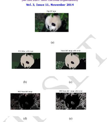
We test our color image segmentation method on natural color images. In Figure 2, part of the procedures of the HSV method is illustrated and final segmentation results are given. Figure 1 (a) includes the original image “panda”. The mean shift on RGB image in Figure 2 (b) , Means shift on HSV image in fig 2(c) and the fig 2(d) and 2(e) display output image with border, we can see that RGB obtains good segmentation results but HSV image does not overlap the look alike region. The sunflower, the flower, is all segmented out separately.. From the point of view for color homogeneity, this result is correct. The computation time of the mean shift segmentation on RGB image and HSV image is given below
(a)
(b) (c)
(d) (e)
Figure (a) is an original image of flower fig. (b) is mean shift segmentation on RGB image fig. (c) is mean shift image on RGB image with border fig. (d) is mean shift segmentation on HSI image fig.(e) mean shift segmented
(a)
(b) (c)
(d) (e)
Figure (a) is an original image of panda fig. (b) is mean shift segmentation on RGB image fig.(c) is mean shift image on RGB image with border fig. (d) is mean shift segmentation on HSI image fig.(e) mean shift segmented
HSI image with border
VII. COMPUTATION TIME TAKEN
Images Mean shift segmentation in RGB image in sec Mean shift in Hsv image
Sunflower 11.90 sec 4.33 sec
Baby 8.711 4.303
Panda 11.546 4.76
VIII. CONCLUSIONS
In this paper, we propose a novel color image segmentation method. We employ the concept of homogeneity, and the mean shift algorithm on HSV image, in our method. Thus the proposed method considers both local and global information in segmenting the image into homogenous regions. We segment the image in the hue-value two dimensional feature space. Thus, the computational complexity is reduced, compared with the methods that segment image in LUV or RGB three-dimensional feature space. The cyclic property of the hue component is considered in the mean shift procedures and in the labelling of the pixels of the image. Experiments show that the proposed method achieves promising results for natural color image segmentation.
REFERENCES
[1] Adams, R. and L. Bischof, “Seeded Region Growing”, IEEE Trans. Pattern Analysis and Machine Intelligence, 1994. [2] Chen, T.Q. and Y. Lu, “Color Image Segmentation--An Innovative Approach” , Pattern Recognition, 2001.
[3] Cheng, H.D., et al., “Color Image Segmentation: Advances and Prospects”, Pattern Recognition, 2001.
[4] Cheng, H.D. and Y.Sun, A Hierarchical Approach to Color Image Segmentation Using Homogeneity” , IEEE Trans. Image Processing, 2000. [5] Cheng, Y., Mean Shift, Mode Seeking, and Clustering”,IEEE Transaction Pattern Analysis and Machine Intelligence, 1995.
[6] Comaniciu, D. and P. Meer,” Robust Analysis of Feature Spaces: Color Image Segmentation” IEEE Conference on Computer Vision and Pattern Recognition, San Juan, Proceeding in, 1997.
[7] Comaniciu, D. and P. Meer,” Distribution Free Decomposition of Multivariate Data.”, Pattern Analysis and Applications, 1999.
[8] Comaniciu, D. and P. Meer, “Mean Shift: A Robust Approach towards Feature Space A Analysis”, IEEE Transaction Pattern Analysis and Machine Intelligence, 2002.
[9] Comaniciu, D., V. Ramesh, and P. Meer. “Real-Time Tracking of Non-Rigid Objects using Mean Shift.” , IEEE Conference on Computer Vision and Pattern Recognition. 2000.
[10] Fukunaga, K. and L.D. Hostetler, “The Estimation of the Gradient of a Density Function, with Applications” IEEE Transaction. Information Theory, 1975.
[11] Iwata, H. and H. Nagahashi, “Active Region Segmentation of Color Image Using Neural Networks”, Systems Computing Journal., 1998. [12] Klinker, G.J., S.A. Shafer, and T. Kanade, “A Physical Approach to Color Image Understanding”, International Journal of Computer Vision, 1990.
[13] Kurugollu, F., B. Sankur, and A.E. Harmani, “Color Image Segmentation Using Histogram Multi thresholding and Fusion”, Image and Vision Computing, 2001..
[14] Nevatia, A Color Edge Detector and Its Use in Scene Segmentation. IEEE Trans. System Man Cybernet, 1977.. [15] Pal, S.K., Image Segmentation Using Fuzzy Correlation. Inform. Sci., 1992.
[16] Silverman, B.W.”Density Estimation for Statistics and Data Analysis”, London: Chapman and Hall 1986.
[17] Sural, S., G. Qian and S. Pramanik. “Segmentation and Histogram Generation Using the HSV Color Space for Image Retrieval”, International Conference on Image Processing (ICIP). 2002:
[18] Torr, P. and D. Murray, “The Development and Comparison of Robust Methods for Estimating the Fundamental Matrix”. International Journal of Computer Vision, 1997.
[19] Wand, M.P. and M. Jones, “Kernel Smoothing”, Chapman & Hall, 1995.
[20] Wang, H. and D. Suter. “A Novel Robust Method for Large Numbers of Gross Errors.”, In Seventh International Conference on Control, Automation, Robotics and Vision (ICARCV02). 2002. Singapore:
[21] Wang, H. and D. Suter. “Variable bandwidth QMDPE and its application in robust optic flow estimation”, International Conference on Computer Vision. Proceedings 2003. France
[22] Zhang, C. and P.Wang “A New Method of Color Image Segmentation Based on Intensity and Hue Clustering”, in International Conference on Pattern Recognition (ICPR). 2000.