Sample Size Determination and Stationarity Testing in the Presence of Trend Breaks

(1)

HUH, SEUNGHO. Sample Size Determination and Stationarity Testing in the Presence of Trend Breaks. (Under the direction of Professor David A. Dickey.)

Traditionally it is believed that most macroeconomic time series represent station-ary fluctuations around a deterministic trend. However, simple applications of the Dickey-Fuller test have, in many cases, been unable to show that major macroeco-nomic variables are stationary univariate time series structure. One possible reason for non-rejection of unit roots is that the simple mean or linear trend function used by the tests are not sufficient to describe the deterministic part of the series. To address this possibility, unit root tests in the presence of trend breaks have been studied by several researchers.

In our work, we deal with some issues associated with unit root testing in time series with a trend break.

The performance of various unit root test statistics is compared with respect to the break induced size distortion problem. We examine the effectiveness of tests based on symmetric estimators as compared to those based on the least squares estimator. In particular, we show that tests based on the weighted symmetric estimator not only eliminate the spurious rejection problem but also have reasonably good power properties when modified to allow for a break.

We suggest alternative test statistics for testing the unit root null hypothesis in the presence of a trend break. Our new test procedure, which we call the “bisection” method, is based on the idea of subgrouping. This is simpler than other methods since the necessity of searching for the break is avoided.

(2)

(3)

(4)

(5)

Biography

(6)

Acknowledgements

I would be grateful to my advisor Dr. Dickey from the bottom of my heart. My research became fruitful thanks to his helpful instruction and advice. Without meeting him, I must have been frustrated in writing this dissertation. He also showed me what a scholar should look like. I was always impressed with his enthusiasm for both teaching and research.

I would like to thank my committee members, Dr. Bhattacharyya, Dr. Gumpertz and Dr. Pantula, for their thoughtful comments and suggestions that greatly im-proved the quality of this dissertation. Another memorable thing during my stay in the department was Dr. Pantula’s devotional concern for students as the Director of Graduate Program.

(7)

List of Tables

2.1 Empirical sizes for Model I using mean adjusted statistics . . . 25

2.2 Empirical sizes for Model I using linear trend adjusted statistics . . . 26

2.3 Empirical sizes for Model I using lagged first differences (Weighted Symmetric estimator) . . . 27

2.4 Empirical sizes for Model II using linear trend adjusted statistics . . . 28

2.5 Empirical powers for Model I using the modified test . . . 29

3.1 Empirical size and power for DGP (3.1) using various subgroups (OLS, n= 100, c= 36) . . . 46

3.2 Empirical size and power for DGP (3.1) using various subgroups (SS, n= 100, c= 37) . . . 48

3.3 Empirical size and power for DGP (3.1) using various subgroups (WS, n= 100, c= 37) . . . 50

3.4 Empirical size and power for DGP (3.1) usingτw and τw∗ . . . 52

3.5 Empirical size and power for DGP (3.1) using various statistics (n = 100, c= 50) . . . 53

3.6 Empirical size and power for DGP (3.1) usingτw,τ and τw,τ∗ . . . 54

3.7 Empirical size and power for DGP (3.2) usingτw,τ and τw,τ∗ . . . 55

3.8 Empirical size and power for DGP (3.2) using various statistics (n = 100, c= 50) . . . 56

3.9 Test results for the unit root null hypothesis . . . 57

4.1 Descriptive information for the stations of interest . . . 99

4.2 Series suggesting higher order model and/or linear trend . . . 101

4.3 Estimates of the lag 1 autoregressive coefficient ρfor each station and target variable . . . 102

4.4 Sample sizes to detect a level shift of size δ=kσ for various values of β and ρ(Method I) . . . 103

4.5 Theoretical and empirical powers for some values of ρ, n and k = 1 using Method II . . . 104

(10)

4.7 Sample sizes for detecting the level shift (k = 1, β =.2, Method II) . 106 4.8 Sample sizes for detecting the level shift (δ= 3, β=.2, Method III) . 107 4.9 Sample sizes for detecting the level shift (k = 1, β = .2, Method I

using t distribution) . . . 108 4.10 Correlation matrix for the 4 variables n1,n2, n3 and n4 in Table 4.6 . 109

4.11 Correlation matrix for the 4 variables n1, n2, n3 and n4 in Table 4.6

(outlying stations excluded) . . . 110 4.12 Principal component vectors for the 4 variables n1, n2, n3 and n4 in

(11)

List of Figures

2.1 Random walk with a break in level (Model I, c = 50) . . . 31 2.2 Empirical sizes for Model I with m= 10 using mean adjusted statistics 32 2.3 Expectations of quadratic forms, their ratios and pivotal statistics (n

= 100) . . . 33 2.4 Empirical sizes for Model I with m = 10 using linear trend adjusted

statistics . . . 34 2.5 Empirical sizes for Model I using lagged first differences (Weighted

Symmetric estimator) . . . 35 2.6 Random walk with a break in drift (Model II, c= 50) . . . 36 2.7 Empirical sizes for Model II with m = 2 using linear trend adjusted

statistics . . . 37 3.1 Empirical size and power for DGP (3.1) using various subgroups (OLS,

n= 100, c= 36) . . . 58 3.2 Empirical size and power for DGP (3.1) using various subgroups (SS,

n= 100, c= 37) . . . 59 3.3 Empirical size and power for DGP (3.1) using various subgroups (WS,

n= 100, c= 37) . . . 60 3.4 Empirical distributions of test statistics (WS, n= 100, c= 75, θ = 5

and ρ=.7; T for τw, M for τ_w∗, L for τw,1 and R for τw,2; M overlays L.) 61

3.5 Empirical size and power of test statistics (WS, n= 100, c= 75 and θ= 5; T for τw, M forτw∗, L forτw,1 and R for τw,2) . . . 62

3.6 Data from a break-in-level model (DGP (3.1),ρ= 0.5,c= 50) . . . . 63 3.7 Data from a break-in-level model (DGP (3.1),ρ= 1, c= 50) . . . 64 3.8 Data from a break-in-slope model (DGP (3.2), ρ= 0.5,c= 50) . . . . 65 3.9 Data from a break-in-slope model (DGP (3.2), ρ= 1, c= 50) . . . 66 3.10 Empirical size and power for DGP (3.1) using τw (1 group) and τw∗ (2

groups) (θ = 2.5, λ=c/n) . . . 67 3.11 Empirical size and power for DGP (3.1) using τw (1 group) and τw∗ (2

(12)

3.12 Empirical size and power for DGP (3.1) using τw (1 group) and τw∗ (2

groups) (θ = 10, λ=c/n) . . . 69

3.13 Empirical size and power for DGP (3.1) using τw,τ (1 group) and τw,τ∗ (2 groups) (θ= 2.5, λ=c/n) . . . 70

3.14 Empirical size and power for DGP (3.1) using τw,τ (1 group) and τw,τ∗ (2 groups) (θ= 5, λ =c/n) . . . 71

3.15 Empirical size and power for DGP (3.1) using τw,τ (1 group) and τw,τ∗ (2 groups) (θ= 10, λ=c/n) . . . 72

3.16 Empirical size and power for DGP (3.2) using τw,τ (1 group) and τw,τ∗ (2 groups) (γ = 0.5,λ =c/n) . . . 73

3.17 Empirical size and power for DGP (3.2) using τw,τ (1 group) and τw,τ∗ (2 groups) (γ = 1, λ=c/n) . . . 74

3.18 Empirical size and power for DGP (3.2) using τw,τ (1 group) and τw,τ∗ (2 groups) (γ = 2, λ=c/n) . . . 75

4.1 Time series data for station 01632000 . . . 113

4.2 Distribution of the descriptive statistics across the stations . . . 114

4.3 Theoretical powers for some values of ρ(Method II) . . . 115

4.4 Comparison of sample sizes between TDM and FDM (triangular weights of length 15; serial numbers in Table 4.1 used for sites) . . . 116

4.5 Comparison of sample sizes between TDM and FDM (flat weights of length 25; serial numbers in Table 4.1 used for sites) . . . 117

4.6 The first two principal components for the 4 variables n1, n2, n3 and n4 in Table 4.6 (outlying stations excluded) . . . 118

4.7 Clustering of the stations by the descriptive statistics (complete link-age) . . . 119

4.8 Clustering of the stations by the sample sizes (single linkage; maximiz-ing CCC) . . . 120

4.9 Clustering of the stations by the sample sizes (single linkage; The largest cluster contains no more than 25 stations.) . . . 121

4.10 Scatter plots of elevation, drainage area and sample size from Method I (k= 1) . . . 122

(13)

Introduction

1.1 Literature review

In the field of time series analysis, there are many good references and textbooks available among which are Priestley (1981), Wei (1990), Box, Jenkins and Reinsel (1994), Hamilton (1994) and Fuller (1996). Of those mentioned, only Box, Jenkins and Reinsel (1994), Hamilton (1994) and Fuller (1996) address the topic of unit roots. The analysis of time series with a unit root became popular following, among others, the work of Dickey (1976). He shows that under the null hypothesis H0 :ρ= 1

in the model Yt = ρYt−1 +et (Y0 = 0, et ∼ N I(0, σ2)), n(ˆρ−1) d

→ 0.5(T2 −₁₎_/G

where ˆρ is the least squares estimator of ρ, T = P∞_i₌₁√2γiUi, G = P∞i=1γi2Ui2, γi = 2(−1)i+1/π(2i−1) and Ui ∼ N I(0,1). Dickey (1976) finds the distribution of n(ˆρµ−1) andn(ˆρτ−1) where ˆρµand ˆρτ are the least squares estimators ofρwhen the fitted model contains a nonzero mean term and a linear trend term respectively. He also tabulates the distribution oft type statistics under the above 3 models. Critical values of these distribuions can be found in Dickey (1976) and Fuller (1996). See Dickey and Fuller (1979) for more information. The random variables T =W(1) and G=R₀1W2₍_t₎_dt_{can be expressed as functionals of a standard Wiener process} _W₍_t_).

(14)

model of unknown ordersp andq. They show that fitting a high order autoregressive model is an appropriate way to test for a unit root in a model of unknown order. Their method is commonly known as the augmented Dickey-Fuller (ADF) test although ADF is also mentioned in Dickey and Fuller (1979) for pure autoregressions..

Gonzalez-Farias (1992) considers maximum likelihood estimation of the param-eters in autoregressive time series. Her paper studies the maximizers of the exact stationary likelihood function when the input data are from a unit root process. She proposes a new unit root test based on these estimators and derives its limiting dis-tribution. Dickey, Hasza and Fuller (1984) discuss the properties of another type of estimator known as the simple symmetric estimator. Park and Fuller (1995) study the weighted symmetric estimator which is another in the class of symmetric estimators. Pantula, Gonzalez-Farias and Fuller (1994) compare the performance of these and other unit root test criteria and determine that the weighted symmetric estimator and the unconditional maximum likelihood estimator provide the most powerful tests against the stationary alternative.

Nelson and Plosser (1982) investigate a collection of important macroeconomic time series asking if they are better characterized as stationary fluctuations around a deterministic trend or as nonstationary processes that have no tendency to return to a deterministic path. They apply the augmented Dickey-Fuller test to 14 ma-jor macroeconomic time series. Their study, which finds that most macroeconomic variables have a univariate time series structure with a unit root, is followed by a series of empirical analyses with similar findings. Several researchers have tried to ex-plain these rather interesting results, believing that most macroeconomic time series represent stationary fluctuations around a deterministic trend.

(15)

root testing and trend breaks are combined by Perron (1989). In the pioneering work of Perron (1989), he considers the null hypothesis that a time series has a unit root with possibly nonzero drift against the alternative that the process is trend stationary. Allowing, under both the null and alternative hypotheses, for the presence of a one-time change in the trend function, Perron (1989) derives test statistics which can distinguish the two hypotheses when such a break is present. He applies these tests to the Nelson and Plosser (1982) data set and rejects the unit root hypothesis for 11 out of the 14 series. He argues that the failure of the usual Dickey-Fuller test to reject the unit root null hypothesis reflects not an actual unit root, but instead that the data are trend stationary around a broken trend. This has come to be called the ‘Perron phenomenon’.

Since Perron assumes the break point is known a priori and treated as exogenous, criticism has emerged from some authors such as Banerjee, Lumsdaine and Stock (1992), Christiano (1992) and Zivot and Andrews (1992).

The most notable of them is Christiano (1992) who argues that the choice of break dates has to be viewed as being correlated with the data. He presents some algorithms for selecting the break date endogenously. A bootstrap approach that takes into account pretest data examination is used to test the null hypothesis of no trend break.

Banerjee, Lumsdaine and Stock (1992) also treat the break date as unknown a priori and suggest recursive and sequential tests of the unit root null hypothesis. Their theoretical results are similar to those of Zivot and Andrews (1992).

Zivot and Andrews (1992) transform Perron’s (1989) unit root test, which is con-ditional on structural change at a known point in time, into an unconcon-ditional unit root test in which the break point is estimated rather than fixed. They check all possible break points and take the minimum t statistic. The data series considered by Perron (1989) are reanalyzed using their estimated break point test statistic.

(16)

structural change. He presents works by himself and many other researchers.

Perron’s (1997) work is closely related to that of Banerjee et al (1992) and that of Zivot and Andrews (1992) in that similar procedures and series are analyzed. He first reexamines his findings from Perron (1989). Unlike his previous study, Perron (1997) assumes that the date of a possible break is not fixed a priori but instead is unknown. He considers various methods to select the break point and the truncation lag parameter. Most of the rejections reported in Perron (1989) are confirmed using his new approach.

Additional tests for a unit root allowing for a break at an unknown time are given by Vogelsang and Perron (1998). They focus on the additive outlier approach where the break is sudden, as opposed to the innovational outlier approach where the change occurs slowly over time.

(17)

1.2 Outline of research

In our work, we concentrate on analyzing time series data with a trend-break. Three somewhat independent papers, Chapters 2, 3 and 4, are related by their focus on the trend-break issue.

In Chapter 2, we compare the performance of various unit root test statistics in the break induced size distortion problem. Leybourne et al (1998) show that, if the data generating process is a random walk with a break near the beginning, standard Dickey-Fuller (1979) tests based on the least squares estimator have serious size distortion. In Chapter 2, we examine the performance of alternative tests based on symmetric estimators. In particular we show that tests based on the weighted symmetric estimator not only eliminate spurious rejection in these problem data sets but also have reasonably good power properties when modified to allow for a break.

In Chapter 3, we suggest alternative test statistics for testing the unit root null hypothesis in the presence of a trend-break. Our new test procedure which we call the “bisection” method is based on the idea of subgrouping. The idea here is to split the data in half and look at the minimum of the resulting two unit root test statistics. This avoids the necessity of searching for the break. It uses all the data in the sense that the minimum is chosen, but clearly is not efficient in its use of the data. We anticipate paying a price in power for a gain in simplicity. Considering some data generating processes, we display empirical size and power results from simulation. We also apply our bisection method to the well-known Nelson and Plosser (1982) data set and compare the results with those of others. The simple bisection method rejects unit roots in several, but not all, of the series for which the more complicated search methods reject.

(18)

(19)

Comparison of Break Induced Size

Distortions among Unit Root Test

Statistics

2.1 Introduction

Recently there has been much interest in testing for a unit root in a time series that has a trend break. Leybourne, Mills and Newbold (1998) study the behavior of standard unit root tests when the data generating process contains a trend break not accounted for by the fitted model. For data consisting of a random walk with a shift in level, they report empirical sizes less than the nominal level when the shift is not too near the beginning of the series. However, if the shift is near the beginning of the series, they report too many rejections of the unit root null hypothesis. Thus a unit root process with an early level shift is too often declared stationary. Leybourne et al (1998) call this the ‘converse Perron phenomenon’ in contrast to the well known ‘Perron phenomenon’ investigated by Perron (1989).

(20)

Gonzalez-Farias and Fuller (1994)), we find that this phenomenon decreases dramat-ically, seeming to disappear in the weighted symmetric case.

In section 2.2, we examine the simple random walk model with a break in level. We consider the simple symmetric estimator ˜ρs and the weighted symmetric estimator

˜

ρw of the lag 1 autoregressive coefficient ρ. Empirical sizes for the pivotal statisticsτs and τw associated with ˜ρs and ˜ρw, respectively, are presented to compare with those

forτµ, the ordinary least squares test statistic. To gain some insight into the empirical

results, we examine the expected values of the quadratic forms constituting the test statistics. This analysis includes τs,τ and τw,τ, the linear trend adjusted versions of τs and τw, respectively, to compare with ττ, the linear trend adjusted version of τµ. An augmented test with lagged first differences is introduced to extend the results to more general cases.

In section 2.3, we consider the random walk model with a break in trend, using τs,τ and τw,τ as test statistics to obtain empirical sizes. The results are compared with those for ττ. Section 2.4 presents some power results for a test based on the weighted symmetric estimator, modified to allow for a break. Finally we make some concluding remarks in section 2.5.

2.2 Data with a break in level

In this section, following Leybourne et al (1998), we consider a data generating process (DGP)

Model I : Yt=mσI(t > c) +Xt, Xt=Xt−1+et, t= 1,2, ..., n

(21)

2.2.1 Using mean adjusted statistics

As in Leybourne et al (1998), to test the unit root null hypothesis, we consider

ˆ ρµ=

Pn

t=2(Yt−Y¯)(Yt−1−Y¯)

Pn

t=2(Yt−1−Y¯)2

(2.1)

which is an ordinary least squares (OLS) estimator∗ of ρ in the non-zero mean first order autoregressive process

Yt=µ+ρYt−1+et. (2.2)

We use, as a test statistic, the associated pivotal statistic

τµ= ˆ ρµ−1

s.e. =

ˆ ρµ−1 q

[Pn_t₌₂(Yt−1−Y¯)2]−1s2

(2.3)

where

s2 = 1 n−3

n X

t=2

[Yt−Y¯ −ρˆµ(Yt−1−Y¯)]2.

Using the test statistic τµ, Leybourne et al (1998) reported the empirical sizes of nominal 5% level tests for various values of break size, m, and break time, c. They found that, asm increases, an increasingly severe phenomenon of ‘spurious rejection’ of the unit root null hypothesis emerges. They also indicated that the earlier is the break, the greater is the rejection rate. Our empirical sizes for τµ are in close agreement with those reported by Leybourne et al (1998).

We consider alternative symmetric estimators ˜ρsand ˜ρw(Fuller, 1996) ofρin (2.2) and their associated pivotal statistics τs and τw. As will be seen, their performance is often quite superior to that of τµ.

For the process (2.2), the simple symmetric (SS) estimator can be written as

˜ ρs=

Pn

t=2ytyt−1

Pn−1

t=2 yt2+ 1₂(y12+yn2)

∗_{This is from the least squares regression of}_Y

t−Y¯ onYt−1−Y¯. The regression ofYton 1,Yt−1

(22)

where yt =Yt−Y¯. The pivotal statistic for the SS estimator is

τs = ˜ ρs−1

s.e. =

˜ ρs−1 q

˜ σ2

s[

Pn−1

t=2 y2t + 1₂(y12+yn2)]−1

(2.4)

where

˜

σ2_s = 1 n−2[

n X

t=2

1

2(yt−ρ˜syt−1)

2₊

n_X−1

t=1

1

2(yt−ρ˜syt+1)

2_]

= 1

n−2[ n X

t=2

(yt−ρ˜syt−1)2+

1 2(1−ρ˜

2

s)(y

2 1−y

2

n)].

The weighted symmetric (WS) estimator for the process (2.2) is

˜ ρw =

Pn

t=2ytyt−1

Pn−1

t=2 yt2+ 1_n

Pn

t=1yt2

(2.5)

and the associated pivotal statistic is

τw = ˜ ρw−1

s.e. =

˜ ρw −1 q

˜ σ2

w(

Pn−1

t=2 yt2+_n1

Pn

t=1yt2)−1

(2.6)

where

˜

σ2_w = 1 n−2[

n X

t=2

wt(yt−ρ˜wyt−1)2+

n_X−1

t=1

(1−wt+1)(yt−ρ˜wyt+1)2]

= 1

n−2[ n X

t=2

(yt−ρ˜wyt−1)2 + (1−ρ˜2w)(y

2 1 − 1 n n X t=1

y_t2)].

and wt= t−_n1 for t= 1,· · ·, n. See Fuller (1996) for detailed discussion of symmetric estimators.

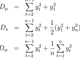
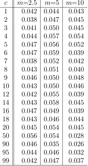
In Table 2.1, we show empirical sizes of nominal 5% level tests using τµ, τs and

τw. We consider the same values of m and c as those used by Leybourne et al

(1998). Simulations are based on 5,000 replications at each (m, c) combination so the standard error of an empirical size is less than q.25/5000 = .007. The sample size per replication is n= 100. Critical values used are those for the mean removed case in Fuller (1996). Data are generated with X0 = 0 so thatX1 =e1 ∼N(0,1).

(23)

τs, the proportion of rejections shows symmetry around c= 50 and gets larger as m increases . The rejection rate is higher for c values in the first or last part than for those in the middle of the data. Theτs rejection rate is much smaller than that ofτµ for early breaks but larger for late breaks.

For τw, the rejection rate is almost invariant to the break size m and shows little size distortion. Most importantly, compared to τµ, τw gives satisfactory performance in that the largest empirical size is around 0.056 (m=5) and most of the others are less than the nominal level 0.05. Figure 2.2 shows empirical sizes of the three tests using mean adjusted statistics for model I withm = 10.

2.2.1.1 Effect of ignoring the break

To obtain some insight into the empirical results, we examine some statistical properties of the test statistics when the break is ignored. As suggested by Amsler and Lee (1995), the asymptotic distributions of the usual Dickey-Fuller tests under ρ = 1 are unaffected by a structural break of fixed size. We now show that this also holds good for the tests based on the symmetric estimators. Thus the spurious rejection problem exists only in finite samples and the effect of ignoring the break may differ between the OLS estimator and the symmetric estimators.

Let xt=Xt−X¯ in Model I where ¯X = 1_n Pn

t=1Xt. Then we know that

¯

Y = ¯X+ (1−λ)m

and

yt =     

xt−(1−λ)m if t≤c=nλ

xt+λm if t > c=nλ.

Recall that the OLS estimator of ρ is

ˆ ρµ=

Pn

t=2ytyt−1

Pn

(24)

and

ˆ

ρµ−1 = Pn

t=2yt−1(yt−yt−1)

Pn

t=2yt2−1

≡ Nµ Dµ

(2.7)

By some straightforward algebra, the numerator of ˆρµ−1 can be written as n

X

t=2

yt−1(yt−yt−1) =

n X

t=2

xt−1(xt−xt−1)−(1−λ)m

nλ_X+1

t=2

et+λm n X

t=nλ+2

et

+mxnλ−(1−λ)m2. Therefore 1 n n X t=2

yt−1(yt−yt−1) =

1 n

n X

t=2

xt−1(xt−xt−1) +Op(

1

√

n). The denominator of ˆρµ−1 can be written as

n X

t=2

y_t2₋₁ = n X

t=2

x2_t₋₁−2m

nλ_X+1

t=2

xt−1+ 2λm

n X

t=2

xt−1

+(1−λ)2m2nλ+λ2m2(n−nλ−1). Using the fact that

1 n2

nλ_X+1

t=2

xt−1 =Op(

1 √ n) and 1 n2 n X t=2

xt−1 =Op(

1 n√n), we have 1 n2 n X t=2

y_t2₋₁ = 1 n2

n X

t=2

x2_t₋₁+Op(√1

n). (2.8)

Combining the results,

n(ˆρµ−1) =

1

n Pn

t=2yt−1(yt−yt−1)

1

n2

Pn

t=2yt2−1

(2.9)

=

1

n Pn

t=2xt−1(xt−xt−1) +Op(√1_n)

1

n2

Pn

t=2x2t−1+Op(√1n)

=

1

n Pn

t=2xt−1(xt−xt−1)

1

n2

Pn

t=2x2t−1

+Op(√1 n)

≡ n(ˆρµ,0−1) +Op(

1

√

(25)

where ˆρµ,0 stands for the OLS estimator of ρ with no break.

Recall that the SS estimator of ρ is

˜ ρs=

Pn

t=2ytyt−1

Pn−1

t=2 yt2+ 12(y

2 1 +yn2) and

˜

ρs−1 = Pn

t=2ytyt−1−

Pn−1

t=2 yt2−

1 2(y

2 1 +yn2) Pn−1

t=2 yt2+1₂(y12+yn2)

= −

1 2

Pn

t=2(yt−yt−1)2

Pn−1

t=2 yt2+1₂(y21+y2n)

≡ Ns Ds

(2.10)

by rearranging the terms in the numerator. The numerator of ˜ρs−1 can be rewritten as −1 2 n X t=2

(yt−yt−1)2 =−

1 2

n X

t=2

(xt−xt−1)2−m(xnλ+1−xnλ)−

m2 2 . Therefore 1 n{− 1 2 n X t=2

(yt−yt−1)2} = −

1 2n

n X

t=2

(xt−xt−1)2 −

m

nenλ+1− m2 2n = 1 n{− 1 2 n X t=2

(xt−xt−1)2}+Op(

1

n). (2.11) We notice that the effect of ignoring the break does not depend on the break time c=nλ here.

Since

y₁2 =x2₁−2(1−λ)mx1 + (1−λ)2m2

and

y2_n=x2_n+ 2λmxn+λ2m2, we can easily show that

1 n2y

2 1 =

1 n2x

2

1 +Op(

1

n√n) and 1 n2y

2

n=

1 n2x

2

n+Op(

1

n√n). (2.12) By (2.8) and (2.12), we have

1 n2{

n_X−1

t=2

y_t2+1 2(y

2 1 +y

2

n)}=

1 n2{

n_X−1

t=2

x2_t + 1 2(x

2 1+x

2

n)}+Op(

1

√

(26)

Combining (2.11) and (2.13),

n(˜ρs−1) =

− 1 2n

Pn

t=2(yt−yt−1)2

1

n2{

Pn−1

t=2 yt2+12(y

2

1+y2n)}

(2.14)

= −

1 2n

Pn

t=2(xt−xt−1)2+Op(1_n)

1

n2{

Pn−1

t=2 x2t +1₂(x21+x2n)}+Op(

1 √ n) = − 1 2n Pn

t=2(xt−xt−1)2

1

n2{

Pn−1

t=2 x2t +1₂(x21+x2n)}

+Op(√1 n)

≡ n(˜ρs,0−1) +Op(

1

√

n) where ˜ρs,0 stands for the SS estimator of ρwith no break.

As to the WS estimator of ρ, we recall that

˜ ρw =

Pn

t=2ytyt−1

Pn−1

t=2 yt2+ 1_n

Pn

t=1yt2

and

˜

ρw−1 = Pn

t=2ytyt−1−Pnt=2−1yt2−

1

n Pn

t=1yt2

Pn−1

t=2 yt2+_n1

Pn

t=1y2t

≡ Nw Dw

. (2.15)

By some straightforward algebra, the numerator of ˜ρw−1 can be written as n

X

t=2

ytyt−1 −

n_X−1

t=2

y_t2− 1 n

n X

t=1

y_t2 =−1 2

n X

t=2

(yt−yt−1)2+

1 2(y

2 1 +y

2

n)−

1 n

n X

t=1

y2_t. By (2.12), we can show that

1 ny 2 1 = 1 nx 2 1+Op(

1

√

n) and 1 ny 2 n= 1 nx 2

n+Op(

1

√

n). (2.16)

Therefore 1 n( n X t=2

ytyt−1−

n_X−1

t=2

y2_t − 1 n

n X

t=1

y_t2) = 1 n{− 1 2 n X t=2

(xt−xt−1)2+

1 2(x

2 1+x

2

n)−

1 n

n X

t=1

x2_t} +Op(√1

n) (2.17)

by (2.8), (2.11) and (2.16). On the other hand,

1 n2(

n_X−1

t=2

y_t2+ 1 n

n X

t=1

y2_t) = 1 n2(

n_X−1

t=2

x2_t + 1 n

n X

t=1

x2_t) +Op(√1

(27)

by (2.8). Combining (2.17) and (2.18),

n(˜ρw−1) =

1

n(

Pn

t=2ytyt−1−

Pn−1

t=2 yt2− 1n

Pn

t=1yt2)

1

n2(

Pn−1

t=2 yt2+n1

Pn

t=1yt2)

(2.19) = 1 n{− 1 2 Pn

t=2(xt−xt−1)2 +1₂(x21+x2n)−

1

n Pn

t=1x2t}+Op(

1

√_n)

1

n2(

Pn−1

t=2 x2t + _n1

Pn

t=1x2t) +Op(√1_n)

=

1

n(

Pn

t=2xtxt−1−

Pn−1

t=2 x2t −

1

n Pn

t=1x2t) +Op(

1

√_n)

1

n2(

Pn−1

t=2 x2t +n1

Pn

t=1x2t) +Op(√1n)

=

1

n(

Pn

t=2xtxt−1−

Pn−1

t=2 x2t −

1

n Pn

t=1x2t)

1

n2(

Pn−1

t=2 x2t +_n1

Pn

t=1x2t)

+Op(√1 n)

≡ n(˜ρw,0−1) +Op(

1

√

n)

where ˜ρw,0 stands for the WS estimator ofρ with no break.

Thus the effect of an added break is Op(1/√n) in all cases with the numerator of n(˜ρs−1) having an even faster convergence rate, Op(1/n).

The studentized test statistics can be written as

τµ = ˆ ρµ−1

s.e. =

n(ˆρµ−1) q

1

n2

Pn

t=2yt2−1

√

s2 (2.20)

= {

n(ˆρµ,0−1) +Op(√1_n)}

q ₁

n2

Pn

t=2x2t−1 +Op(√1_n)

√

s2

≡ τµ,0 +Op(

1

√

n),

τs = ˜ ρs−1

s.e. =

n(˜ρs−1) q

1

n2{

Pn−1

t=2 yt2+1₂(y12+yn2)}

q ˜ σ2 s (2.21) = {

n(˜ρs,0−1) +Op(√1_n)}

q₁

n2{

Pn−1

t=2 x2t +1₂(x21+x2n)}+Op(

1 √ n) q ˜ σ2 s

≡ τs,0+Op(

1

√

n) and

τw = ˜ ρw−1

s.e. =

n(˜ρw−1) q

1

n2(

Pn−1

t=2 yt2+ _n1

Pn

t=1yt2)

q ˜ σ2

w

(28)

= {n(˜ρw,0−1) +Op(

1

√

n)}

q

1

n2(

Pn−1

t=2 x2t +_n1

Pn

t=1x2t) +Op(√1_n)

q ˜ σ2

w

≡ τw,0+Op(

1

√

n)

where τµ,0, τs,0 and τw,0 represent the test statistics with no break. We use the fact

that s2_{, ˜}_σ2

s and ˜σ2w are consistent regardless of the break under ρ= 1.

Although the effect of ignoring the break in the numerator of n(˜ρs−1) is Op(1_n), the effect is Op(√1

n) in all of the studentized test statistics. The spurious rejection problem disappears at the same rate for all tests, asn becomes larger.

2.2.1.2 Analysis of expectations

We next analyze the expectations of the quadratic forms constituting the test statistics to gain some more clues with respect to the empirical results. These are only clues, as the power also depends on the shapes of the distributions’ tails.

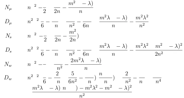
Define ˆρµ−1≡Nµ/Dµ, ˜ρs−1≡Ns/Ds and ˜ρw−1≡Nw/Dw. Some straightfor-ward but tedious algebra gives

E[Nµ] = nσ2[−1 2 +

1 2n−

m2₍₁₋_λ₎

n ]

E[Dµ] = n2σ2[1 6 −

1 3n+

1 3n2 −

1 6n3 +

m2λ(1−λ)

n −

m2λ2 n2 ]

E[Ns] = nσ2(−1 2 +

1 2n−

m2

2n) E[Ds] = n2σ2[1

6 − 1 3n+

1 3n2 −

1 6n3 +

m2_λ₍₁−_λ₎

n −

m2_λ2₊_m2₍₁−_λ₎2

2n2 ]

E[Nw] = nσ2[−1 3 +

1 3n2 −

2m2λ(1−λ)

n ]

E[Dw] = n2σ2[(1 6 −

2 3n +

5 6n2 −

1 3n3)(

n+ 1 n ) +

2 3n2 −

1 n3 +

1 3n4

+m

2_λ₍₁₋_λ₎₍_n_{+ 1)}₋_m2_λ2₋_m2₍₁₋_λ₎2

n2 ]

where λ=c/nis the proportion of observations before the break.

(29)

The expectations of the denominators above are concave functions of λ and sym-metric around λ = 0.5. They are very similar as we can see in the second column of Figure 2.3. This is expected because the denominators can be written as

Dµ =

n_X−1

t=2

y2_t +y2₁

Ds =

n_X−1

t=2

y2_t + 1 2(y

2 1 +y

2

n)

Dw =

n_X−1

t=2

y2_t + 1 n

n X

t=1

y_t2

The major differences are in the numerators. E[Nµ] is an increasing function of λ and E[Ns] does not depend on λ. E[Nw] is a convex function of λ and symmetric around λ = 0.5. Notice that lower values of the numerators suggest higher rates of rejecting H0 :ρ= 1 as we are using left tailed tests.

If we consider the ratio of the expectations of the numerators and the denomi-nators, E[Nµ]/E[Dµ] is a concave function of λ which is negative and not symmetric around λ = 0.5. Its absolute value is larger for λ near 0 than for λ near 1. As λ increases from 0 to 1, its absolute value decreases at first and then increases. This corresponds to the empirical results of high τµ rejection rates for early breaks.

E[Ns]/E[Ds] is a symmetric concave function ofλ. Its absolute values are larger for

λ near 0 or 1 than forλ near 0.5. E[Nw]/E[Dw] is also a symmetric concave function of λ, becoming nearly constant as n increases. The absolute values of E[Ns]/E[Ds] are much larger than those of E[Nw]/E[Dw] for λ near 0 or 1.

This also corresponds to the empirical results that τs and τw show symmetry around λ= 0.5 with τs giving higher rejection rates thanτw for λ near 0 or 1.

All three standard errors in (2.3), (2.4) and (5.1) are of the form

s.e. = s

MSE D

(30)

standard error, a.s.e., as

a.s.e. ≡ v u u t σ2

E[D].

We find that a.s.e. is a symmetric convex function ofλ and that (E[Nµ]/E[Dµ])/a.s.e. and (E[Ns]/E[Ds])/a.s.e. show similar shapes to E[Nµ]/E[Dµ] and E[Ns]/E[Ds] re-spectively.

On the other hand, (E[Nw]/E[Dw])/a.s.e. has a little different shape from that of E[Nw]/E[Dw]. The former is convex whereas the latter is nearly flat but concave. These graphs are displayed as ‘pivotal statistics’ in the right column of Figure 2.3.

2.2.2 Using linear trend adjusted statistics

Leybourne et al (1998) also considered ˆρτ which is the OLS estimator ofρ in the model

Yt=µ+βt+ρYt−1 +et. (2.23) Alternatively the first order autoregressive model around a linear trend can be written as

Yt−µ−βt=ρ[Yt−1−µ−β(t−1)] +et. (2.24) By simple algebra, the model (2.24) becomes

Yt = [µ(1−ρ) +βρ] +β(1−ρ)t+ρYt−1+et

≡ γ0+γ1t+ρYt−1+et

which is the same model as (2.23). We denote the pivotal statistic associated with ˆρτ asττ. ˆρτ and ττ can be obtained if we replace (Yt−Y¯) with (Yt−ˆa−ˆbt) in (2.1) and (2.3), respectively, where ˆa and ˆb are OLS estimates of a and b in the simple linear regression

(31)

Leybourne et al (1998) found that ττ gives a similar size distortion pattern to that of τµ when Model I is used to generate the data. Our empirical sizes for ττ in Table 2.2 are in close agreement with theirs. The magnitude of the spurious rejection problem is more severe for ττ than forτµ for the smallestλ. The problem evaporates more rapidly for ττ than for τµ asλ increases.

Denote the linear trend adjusted versions ofτsandτw asτs,τ andτw,τ respectively. τs,τ and τw,τ can be obtained from (2.4) and (2.5), respectively, by replacing (Yt−Y¯) with the residual from (2.25). Empirical sizes for τs,τ and τw,τ are given in Table 2.2. In the simulation, the number of replications is 5,000 and the sample size per replication is n = 100. Critical values used are those for the linear trend removed case in Fuller (1996).

As in the mean adjusted cases in section 2.2.1, the spurious rejection problem is less severe for τs,τ and τw,τ than for ττ. Also τs,τ and τw,τ show similar patterns of empirical sizes to τs and τw, respectively. τs,τ gives a slightly higher rejection rate

than τs. Like τw, τw,τ gives satisfactory performance and retains size close to the

nominal 5% level. Figure 2.4 displays the empirical sizes for model I withm = 10 for the linear trend adjusted statistics.

2.2.3 Using lagged first differences

To extend the results for the first order process to more general processes, we consider an augmented test based on the WS estimator since it shows better perfor-mance than the other estimators in the previous results. We introduce lagged first differences as in the usual Augmented Dickey-Fuller test based on the OLS estimator. Our test statistic is denoted asτw,a.

Using the data arrangement and weights in Table 10.1.1, Fuller (1996), withp= 2, we perform the weighted regression estimation of the autoregressive model written as

(32)

where Zt−1 =Yt−1−Yt−2. For reference, we reproduce the table for p= 2 here.

Weight Dependent Variable θ1 θ2

w3 Y3 Y2 Y2−Y1

w4 Y4 Y3 Y3−Y2

..

. ... ... ...

wn Yn Yn−1 Yn−1−Yn−2

1-wn−1 Yn−2 Yn−1 Yn−1−Yn 1-wn−2 Yn−3 Yn−2 Yn−2−Yn−1

..

. ... ... ...

1-w2 Y1 Y2 Y2−Y3

The estimator of θ= (θ1, θ2)0 can be obtained as

ˆ

θ = (˜θ1,θ˜2)0 = (X0W X)−1X0W Y

where X is the (2n−2p)×p matrix below the headings θ1, θ2 in the table, Y is

the (2n−2p)-dimensional column vector called the dependent variable andW is the (2n−2p) diagonal matrix whose elements are given in the “Weight” column. The hypothesis of a unit root is tested by testing the hypothesis that θ1 = 1. Then the

test statistic τw,a can be written as

τw,a= ˜ θ1−1

s.e. (2.26)

whose limiting distribution, using the proper s.e., is the same as that of τw in (5.1). Because each observation gives rise to 2 rows in Fuller’s Table, the standard error printed by a typical regression package needs to be multiplied by √2 in (2.26) in order to use the critical values from Fuller (1996).

(33)

2.3 Data with a break in trend

In this section, we consider another DGP

Model II : Yt=Yt−1+mσI(t > c) +et, t= 1,2, ..., n

where the et are normal independent (0,σ2) random variables and we can assume σ = 1 without loss of generality as in Model I. This model corresponds to ‘Model (B) under the null hypothesis’ of Perron (1989). Since Model II can be rewritten as

Yt = Yt−1+et, t = 1,· · ·, c Yt = Yt−1+m+et

= Yc+m(t−c) + t X

j=c+1

ej, t=c+ 1,· · ·, n, (2.27)

it might be called a random walk with a break in drift where mI(t > c) is the drift parameter. When m 6= 0, the time trend will dominate the long-run behavior of Yt in (2.27) because Pt_j₌_c₊₁ej = Op(

√

n) and hence Pt_j₌_c₊₁ej is small in probability relative to t. Therefore we consider the linear trend adjusted versions of statistics to test the unit root null hypothesis. Time series data generated from Model II with various values ofm are displayed in Figure 2.6.

Leybourne et al (1998) reported empirical sizes for Model II using the test statistic

ττ. Columns labelled ττ in Table 2.4 contain our empirical sizes forττ, which are close

to those of Leybourne et al (1998). They found that, as m increases, the range of values of λfor which serious problems are found increases. They also concluded that frequent spurious rejections of the null hypothesis occur for low values of λ but the pattern for Model II is a little different than that for Model I. The spurious rejection problem was most severe for the lowest values of λin Model I. In contrast, for Model II, it increases at first in severity with increasing λ, but then rapidly diminishes as λ increases further.

(34)

by Leybourne et al (1998). These results are also presented in Table 2.4. We notice that, for Model II,τs,τ and τw,τ give similar patterns of empirical sizes to each other. Although they do not show size distortion problems, they are severely undersized for a wide range ofcwhich might suggest lower power against the alternative hypothesis. We comment on this in section 2.4. As far as spurious rejection is concerned, τw,τ again presents much better empirical sizes thanττ. Empirical sizes for Model II with m= 2 are shown in Figure 2.7.

2.4 Empirical powers allowing for a break

Thus far we have considered the effects of ignoring an existing break and have found the weighted symmetric estimator performs well, avoiding spurious declarara-tions of stationarity. If a series consists of a level shift plus stationary errors and one tests for stationarity without modelling the level shift, it is unclear whether accepting or rejecting the null hypothesis is desirable - neither is correct so power should not be a concern here. However, if we modified the WS estimator to accomodate a model with a break, we would want that test to have good power. We investigate this now. LetDtbe a dummy variable representing a structural break, that isDt=I(t > c). We first perform regression estimation of the model

Yt =β0+β1Dt+et

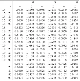
and produce the residuals rt = Yt−Yˆt = Yt−βˆ0 −βˆ1Dt. Replacing (Yt−Y¯) with rt in (2.5) and (2.6), we obtain a WS estimator and associated pivotal statistic, respectively, allowing for a break. For the limiting distribution of these statistics, see Appendix A.

Table 2.5 presents empirical size and power results with respect to Model I as a DGP. Various values of n, λ and ρ are used where λ = c/n is the break time in

(35)

for the modified estimator whether there is a break or not in the DGP. Both critical values from a simulation method and from Fuller (1996) are applied. The number of replications is 1,000.

For all values of n, empirical sizes (ρ= 1) are too big if we use the critical values from Fuller (1996). This is no surprise since most previous research on trend breaks shows that critical values must be adjusted for breaks. For instance, Perron (1989) showed that the critical values under various models are noticeably smaller than the standard Dickey-Fuller critical value.

The values for τw with no fitted break are shown under the label λ= 0 in Table 2.5. Previous researchers have used least squares estimation for trend break cases and, in Table 2.5, we include with underlines the powers obtained using OLS estimation. See Tables 4-6 in Pantula et al (1994) for the empirical powers of τµ andτw when no break is present.

Using critical values from simulation, we obtain reasonably good empirical powers. For givennandρ, as λchanges from .02 to .5, the power decreases. In general, when there really is no break, the modified test that is invariant to breaks gives less power than τw with no fitted break. When there is a break (λ > 0), the modified test based on the WS estimator gives better power than the modified test based on the OLS estimator. It is seen that substantial improvement in power occurs with the WS estimator especially for larger λ values.

2.5 Conclusion

(36)

The WS estimator in particular shows practically no size distortion and, even for large m, nearly retains the nominal level. The performance of the WS estimator in the augmented case is as good as in the simple case. The WS estimator also generates reasonably good empirical power when modified to allow for a break.

(37)

Table 2.1: Empirical sizes for Model I using mean adjusted statistics

m=2.5 m=5 m=10

c τµ τs τw τµ τs τw τµ τs τw

(38)

Table 2.2: Empirical sizes for Model I using linear trend adjusted statistics

m=2.5 m=5 m=10

c ττ τs,τ τw,τ ττ τs,τ τw,τ ττ τs,τ τw,τ

(39)

Table 2.3: Empirical sizes for Model I using lagged first differences (Weighted Sym-metric estimator)

c m=2.5 m=5 m=10

(40)

Table 2.4: Empirical sizes for Model II using linear trend adjusted statistics

m=0.5 m=1 m=2

c ττ τs,τ τw,τ ττ τs,τ τw,τ ττ τs,τ τw,τ

(41)

Table 2.5: Empirical powers for Model I using the modified test

n= 50 n= 100

ρ λ=0 .02 .05 .25 .50 λ=0 .02 .05 .25 .50

CV∗ -2.57 -2.89 -2.94 -3.26 -3.31 -2.55 -2.85 -2.95 -3.18 -3.26 1.00 0.05 0.05 0.05 0.05 0.05 0.05 0.05 0.05 0.05 0.05 0.05† 0.05 0.05 0.05 0.05 0.05 0.05 0.05 0.05 0.05 0.95 0.12 0.10 0.10 0.08 0.09 0.26 0.17 0.15 0.13 0.14 0.07 0.10 0.10 0.07 0.07 0.12 0.17 0.15 0.11 0.10 0.90 0.25 0.18 0.16 0.13 0.14 0.60 0.45 0.39 0.33 0.32 0.12 0.18 0.16 0.10 0.09 0.31 0.45 0.39 0.25 0.22 0.80 0.58 0.45 0.42 0.32 0.32 0.98 0.94 0.91 0.85 0.83 0.32 0.45 0.42 0.25 0.22 0.88 0.94 0.91 0.75 0.68

0.50 0.99 0.99 0.97 0.96 1.00 1.00 1.00 1.00

0.99 0.99 0.94 0.90 1.00 1.00 1.00 1.00

CV‡ -2.57 -2.55

1.00 0.10 0.11 0.19 0.23 0.11 0.12 0.20 0.23

0.95 0.21 0.21 0.29 0.35 0.32 0.33 0.41 0.48

0.90 0.33 0.33 0.42 0.49 0.66 0.66 0.74 0.77

0.80 0.66 0.67 0.73 0.76 0.99 0.99 0.99 0.99

0.50 1.00 1.00 1.00 1.00 1.00 1.00 1.00 1.00

∗_{Critical values are from Fuller (1996) for}_λ_{=0 or from simulation otherwise.} †_{Underlined values are from the OLS estimator.}

(42)

Table 2.5: continued

n= 250

ρ λ=0 .02 .05 .25 .50

CV∗ -2.54 -2.82 -2.87 -3.11 -3.20 1.00 0.05 0.05 0.05 0.05 0.05 0.05† 0.05 0.05 0.05 0.05 0.95 0.78 0.61 0.58 0.49 0.46 0.44 0.61 0.57 0.35 0.30 0.90 0.99 0.99 0.99 0.97 0.96 0.97 0.99 0.99 0.90 0.86 0.80 1.00 1.00 1.00 1.00 1.00 1.00 1.00 1.00 1.00 1.00

0.50 1.00 1.00 1.00 1.00

1.00 1.00 1.00 1.00 CV‡ -2.54

1.00 0.10 0.12 0.19 0.22

0.95 0.80 0.80 0.85 0.88

0.90 1.00 1.00 1.00 1.00

0.80 1.00 1.00 1.00 1.00

0.50 1.00 1.00 1.00 1.00

∗_{Critical values are from Fuller (1996) for}_λ_{=0 or from simulation otherwise.} †_{Underlined values are from the OLS estimator.}

(43)

t

Y

0 20 40 60 80 100

-5

0

5

10

15

m= 0

t

Y

0 20 40 60 80 100

-25

-20

-15

-10

-5

0

m= 2.5

t

Y

0 20 40 60 80 100

-15

-10

-5

m= 5

t

Y

0 20 40 60 80 100

-12

-8

-6

-4

-2

0

m= 10

(44)

C

Empirical Size

0 20 40 60 80 100

0.0

0.1

0.2

0.3

0.4

0.5

Least Squares Simple Symmetric Weighted Symmetric

(45)

Lambda

E[num]

0.0 0.4 0.8

-55 -50 -45 -40 -35 OLS SS WS E[num] m=2.5 Lambda E[den]

0.0 0.4 0.8

1650 1700 1750 E[den] m=2.5 Lambda E[num]/E[den]

0.0 0.4 0.8

-0.034 -0.030 -0.026 -0.022 E[num]/E[den] m=2.5 Lambda Tau

0.0 0.4 0.8

-1.4 -1.2 -1.0 Pivotal Statistics m=2.5 Lambda E[num]

0.0 0.4 0.8

-70 -60 -50 -40 m=5 Lambda E[den]

0.0 0.4 0.8

1600 1800 2000 2200 m=5 Lambda E[num]/E[den]

0.0 0.4 0.8

-0.045 -0.035 -0.025 m=5 Lambda Tau

0.0 0.4 0.8

-1.8 -1.6 -1.4 -1.2 -1.0 -0.8 m=5 Lambda E[num]

0.0 0.4 0.8

-100 -80 -60 -40 m=7.5 Lambda E[den]

0.0 0.4 0.8

2000 2500 3000 m=7.5 Lambda E[num]/E[den]

0.0 0.4 0.8

-0.06 -0.05 -0.04 -0.03 -0.02 m=7.5 Lambda Tau

0.0 0.4 0.8

-2.5 -2.0 -1.5 -1.0 m=7.5 Lambda E[num]

0.0 0.4 0.8

-140 -100 -80 -60 -40 m=10 Lambda E[den]

0.0 0.4 0.8

1500 2000 2500 3000 3500 4000 m=10 Lambda E[num]/E[den]

0.0 0.4 0.8

-0.08 -0.06 -0.04 -0.02 m=10 Lambda Tau

0.0 0.4 0.8

-3.5

-2.5

-1.5

m=10

(46)

C

Empirical Size

0 20 40 60 80 100

0.0

0.2

0.4

0.6

(47)

C

Empirical Size

0 20 40 60 80 100

0.03

0.04

0.05

0.06

m=2.5 m=5 m=10

(48)

t

Y

0 20 40 60 80 100

-10

-8

-6

-4

-2

0

2

m= 0

t

Y

0 20 40 60 80 100

-5

0

5

10

15

m= 0.5

t

Y

0 20 40 60 80 100

0

1

02

03

04

05

0

m= 1

t

Y

0 20 40 60 80 100

0

2

04

06

08

0

m= 2

(49)

C

Empirical Size

0 20 40 60 80 100

0.0

0.2

0.4

0.6

0.8

(50)

Alternative Method for Testing the

Unit Root Null Hypothesis in the

Presence of a Break

3.1 Introduction

Since the pioneering work by Perron (1989), many researchers have been interested in testing for a unit root in time series with a trend-break. It is known that power decreases in finite samples as the trend-break becomes larger when the usual Dickey-Fuller (1979) test is used.

(51)

(1992). They checked all possible break points and took the minimum t statistic. In this Chapter, we present an alternative test statistic for testing the unit root hypothesis allowing for a possible trend break. Although our method assumes that the break time is unknown, it is ignored rather than estimated. Using the new test statistic, we perform a Monte Carlo simulation to obtain its empirical powers which are rather invariant to the break size.

Section 3.2 describes the idea of subgrouping and simulation results to find the optimal number of subgroups. As a result, we suggest new test statistics in section 3.3. Section 3.4 presents the data generating processes and some empirical power results from a Monte Carlo simulation. In section 3.5, we apply our test procedure to the real data analyzed originally by Nelson and Plosser (1982). We finally make concluding remarks in section 3.6.

3.2 Subgrouping of data

Our new test procedure is based on the idea of dividing the whole data into some subgroups of the same size. For each subgroup, a certainttype statistic is calculated. Then the minimum of all these statistics is defined as a new test statistic for the unit root null hypothesis in time series with a break.

Suppose we have stationary series around a broken trend. After dividing the data into subgroups, we expect to have a smaller value of the test statistic from a subgroup without a break than from another subgroup with a break. Therefore taking the minimum among all the statistics might give us reasonable power as we are using left tailed tests. This is a key motivation for our subgrouping idea.

The approach by Perron (1989) assumes the break point is known a priori. Using dummy variables, he combines the data before the break with the data after the break. We do not have to assume a known break point in our new procedure.

(52)

break point that gives the least favorable result for the unit root null hypothesis. Then they take the t type statistic giving that break point. Our procedure is simpler because it does not consider estimating the unknown break point.

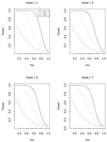
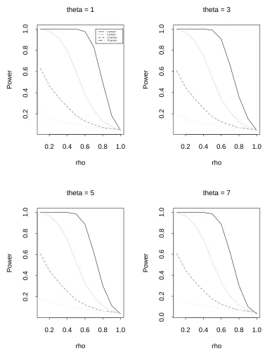
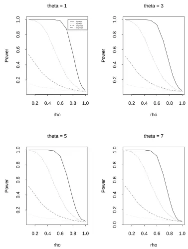
We perform some simulations to decide the optimal number of subgroups. The data generating process given by (3.1) in section 3.4 is used for various numbers of subgroups. We considern(ˆρ−1) type statistics from the ordinary least squares (OLS) estimator, the simple symmetric (SS) estimator and the weighted symmetric (WS) estimator. The number of replications is 5,000 and the sample size per replication is n= 100. We consider the break point c= 36 (for OLS) or c= 37 (for SS and WS) and the break size θ = 1, 3, 5 and 7. In Tables 3.1-3.3 and Figures 3.1-3.3, we show empirical size and power results from simulation.

Clearly the optimal number of subgroups is 2. We expect similar results for t type statistics. The next section describes our new test procedure which we call the “bisection” method.

3.3 Bisection method

From the previous work by Leybourne et al (1998) and Huh and Dickey (1999), we know that, in the presence of an early break, the conventional Dickey-Fuller (1979) test based on the least squares estimator can be subject to serious size distortion but tests based on the weighted symmetric estimator cure this problem. Therefore our bisection method in this Chapter is based on the WS estimator of ρ, ˜ρw, and the associated pivotal statistic τw in the non-zero mean AR(1) process

Yt=µ+ρYt−1+et. Our new bisection test statistic is defined as

(53)

where τw,k is τw for subgroup k for k = 1,2. Each subgroup is supposed to have the same number of observations. Note that we are dealing with the mean adjusted case. See Appendix B for the limiting distribution of τ_w∗. Figure 3.4 shows empirical distributions of τ_w∗, τw,1, τw,2 and the usual τw associated with the data generating process (3.1) in section 3.4. We assume n = 100, c = 75, θ = 5 and ρ =.7. Notice that the empirical distributions of τw,1 and τw∗ are very close to each other since the break is in the second subgroup (c= 75). That does not necessarily mean that they have the same power for a certain ρbecause the critical values are different as shown in Figure 3.4. In the figure, the vertical line on the left denotes the critical value for τ_w∗, so the power for τ_w∗ is lower than that forτw,1 as can be seen in Figure 3.5. This

generally holds good for other values of ρ.

As to the linear trend adjusted case, we consider the WS estimator of ρ and the associated pivotal statistic τw,τ in the model

Yt=µ+βt+ρYt−1 +et.

τw,τ can be regarded as the linear trend adjusted version ofτw. We then use τw,τ∗ , the minimum of two τw,τ statistics, as a new test statistic. See Huh and Dickey (1999) for more details about τw and τw,τ.

3.4 Empirical size and power results

In this section, we display some size and power simulation results using bisection test statistics.

We consider two data generating processes (DGPs) given by

(54)

toσ. Notice that DGP (3.1) corresponds to a break-in-level model with levels 0 and θσ and DGP (3.2) to a break-in-slope model with slopes 0 and γσ. Figures 3.6-3.9 present some typical time series data generated from DGPs (3.1) and (3.2).

We perform a Monte Carlo simulation for some values of θ, γ, c and ρ. The number of replications is 5,000 and the sample size per replication is n= 100. The critical values for τ_w∗ and τ_w,τ∗ are also calculated by simulation.

3.4.1 Data with a break in level

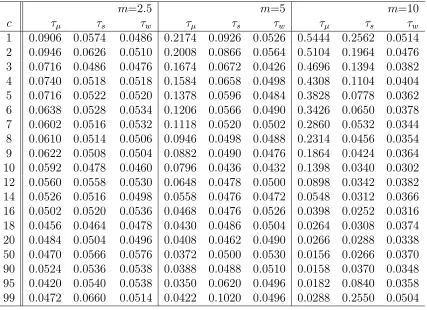
3.4.1.1 Mean adjusted case

For DGP (3.1), we first use the mean adjusted statistics τw and τw∗. As might be expected from our Chapter 2 results, neither τw nor τw∗ show size distortion for DGP (3.1).

If we use τ_w∗ as a test statistic, the powers are in general higher than those for the usualτw when there is a break. Some exceptions are for the early break (c= 1) or the late break (c = 99). For given ρ, the powers for τ_w∗ are relatively invariant whereas those for the usual τw decrease dramatically asθ becomes larger.

If there is no break (θ= 0), on the other hand, the usualτw is more powerful than τ_w∗. This is so especially for large values ofρ. Notice that our power results for τw in Table 3.4 agree closely with those of Pantula et al (1994).

Table 3.4 and Figures 3.10-3.12 present the empirical size and power results for DGP (3.1) usingτw andτw∗. As might be expected,τw outperformsτw∗ for small breaks andτ_w∗ outperformsτw for larger breaks. In all cases, τw∗ is more uniform with respect toλ.

We compare the size and power properties of our test procedure with those of Vogelsang and Perron (1998). They consider a DGP

Yt = θI(t > Tbc) +γ(t−T c

b)I(t > T c

b) +Zt,

(55)

whereet∼N I(0,1) andTbcstands for the true break date. Withα=ψ =γ = 0, DGP (3.3) is exactly the same as our DGP (3.1). They introduce 4 different test statistics

(Tb(tα),ˆ Tb(|tγˆ|),Tb(tˆγ) and Tb(F_θ,ˆ_γ_ˆ)) according to the methods of estimating the true

break date. For their simulation, n= 100 and Tc

b = 50. When ρ =.8, our τw∗ shows higher power than most of their statistics regardless of the break sizeθ. Although one statistic (Tb(tα)) withˆ θ = 10 has higher power than our τw∗, that can be attributed to its size distortion problem. In Table 3.5, we show empirical powers for DGP (3.1) using various statistics.

3.4.1.2 Linear trend adjusted case

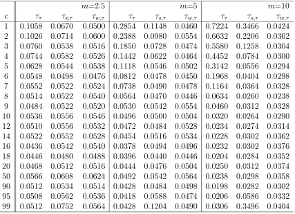
We next use the linear trend adjusted statisticsτw,τ and τw,τ∗ for DGP (3.1). Both τw,τ and τw,τ∗ retain empirical sizes (ρ= 1) close to the nominal 5% significance level. When there is no break, τw,τ shows higher power than τw,τ∗ for given ρ. Notice also thatτw,τ and τw,τ∗ generate lower power than τw and τw∗ respectively.

When the break is fairly big (θ = 10), the powers for τ_w,τ∗ are generally higher than those for τw,τ. As in the mean adjusted case, the powers for τ_w,τ∗ are relatively invariant compared with those forτw,τ.

The empirical size and power results using τw,τ and τw,τ∗ are presented in Table 3.6 and Figures 3.13-3.15.

3.4.2 Data with a break in slope

For DGP (3.2) which represents a break-in-slope model, we adopt the linear trend adjusted statistics τw,τ and τw,τ∗ . Even though both τw,τ and τw,τ∗ retain the nominal 5% significance level, τw,τ becomes severely under-sized asγ grows larger.

(56)

The simulation results for DGP (3.2) using τw,τ and τw,τ∗ are displayed in Table 3.7 and Figures 3.16-3.18.

To compare with the results of Vogelsang and Perron (1998), we consider DGP (3.3) with α=ψ =θ = 0 which is exactly the same as our DGP (3.2). When ρ=.8, the powers of our τ_w,τ∗ are as good as those of their statistics for some values of γ. Power comparisons between τ_w,τ∗ and statistics of Vogelsang and Perron (1998) are displayed in Table 3.8.

3.5 Empirical applications

We now apply our bisection method to the data set analyzed originally by Nelson and Plosser (1982). The data set consists of 14 major macroeconomic time series which include measures of output, spending, money, prices and interest rates. The data are annual, generally averages for the year, with starting dates from 1860 to 1909 and ending in 1970 in all cases. We analyze the natural logarithm of all the data except for the interest rate series, which is analyzed in levels form. Many researchers have referred to this data set. See Nelson and Plosser (1982) for more details about the data set.

In Table 3.9, we compare our unit root test results with those of Nelson and Plosser (1982), Perron (1989), Zivot and Andrews (1992) and Perron (1997). Numbers are the values of the test statistics.

Nelson and Plosser (1982) apply the usual Dickey-Fuller test with extra lags of the first differences of the data (augmented Dickey-Fuller test). Methods of Perron (1989) and Zivot and Andrews (1992) are briefly described in section 3.2. Perron (1997) is closely related to and complements Zivot and Andrews (1992) in that similar procedures are analyzed. See the original articles for more details.

(57)

to some selection criteria. Nelson and Plosser (1982) use critical values from Fuller (1996) whereas the other methods, including ours, use their own critical values gen-erated from simulation. Our bisection method using τ_w,τ∗ rejects the unit root null hypothesis atα=.05 for the series “Real GNP”, “Real per capita GNP”, “Industrial production”, “Unemployment rate”, “Real wages” and “Money stock”.

3.6 Summary

In this work, we suggest new test statistics τ_w∗ and τ_w,τ∗ for testing the unit root null hypothesis in the presence of a trend break. These statistics are based on the idea of dividing the data into subgroups of the same size. The optimal number of subgroups turns out to be 2.

Our bisection method can be used without assuming a known break point unlike Perron’s (1989) original approach. It is simpler than the methods of Zivot and An-drews (1992) and Perron (1997). When there is a trend-break and the break size is fairly big, the empirical powers of the new statistics are in general higher than the usual τw and τw,τ respectively. Based on simulation studies, the power properties of our test procedure are as good as those of Vogelsang and Perron’s (1998).

(58)

Table 3.1: Empirical size and power for DGP (3.1) using various subgroups (OLS, n= 100, c= 36)

No. of subgroups 1 2 5 10 20

(59)

(60)

Table 3.2: Empirical size and power for DGP (3.1) using various subgroups (SS, n= 100, c= 37)

(61)

(62)

Table 3.3: Empirical size and power for DGP (3.1) using various subgroups (WS, n= 100, c= 37)

(63)

(64)

Table 3.4: Empirical size and power for DGP (3.1) using τw and τw∗

θ = 0 θ= 5 θ = 10

ρ c τw τw∗ τw τw∗ τw τw∗

(65)

Table 3.5: Empirical size and power for DGP (3.1) using various statistics (n= 100, c= 50)

ρ 1 0.8

θ 0 5 10 0 5 10

Tb(tα)ˆ † 0.040 0.108 0.507 0.295 0.435 0.861

Tb(|tˆγ|)† 0.049 0.048 0.032 0.301 0.098 0.042 Tb(tˆγ)† 0.050 0.050 0.040 0.350 0.133 0.055

Tb(F_θ,ˆ_ˆ_γ)† 0.052 0.050 0.020 0.339 0.194 0.163

τ_w∗ 0.050 0.048 0.050 0.599 0.592 0.596

(66)

Table 3.6: Empirical size and power for DGP (3.1) using τw,τ and τw,τ∗

θ = 0 θ= 5 θ = 10

(67)

Table 3.7: Empirical size and power for DGP (3.2) using τw,τ and τw,τ∗

γ = 0 γ = 1 γ = 2

(68)

Table 3.8: Empirical size and power for DGP (3.2) using various statistics (n= 100, c= 50)

ρ 1 0.8

γ 0 1 2 0 1 2

Tb(tα)ˆ † 0.040 0.044 0.076 0.295 0.236 0.386

Tb(|tˆγ|)† 0.049 0.036 0.032 0.301 0.239 0.230 Tb(tˆγ)† 0.050 0.072 0.061 0.350 0.376 0.371

Tb(F_θ,ˆ_ˆ_γ)† 0.052 0.027 0.021 0.339 0.193 0.184

τ_w,τ∗ 0.050 0.050 0.052 0.306 0.298 0.302

(69)

Table 3.9: Test results for the unit root null hypothesis

Series n N&P‡ P1§ Z&A¶ P2k Bisection∗∗ Real GNP 62 -2.99 -5.03∗ -5.58∗ -5.93∗ -4.09† Nominal GNP 62 -2.32 -5.42∗ -5.82∗ -8.16∗ -2.28 Real per capita GNP 62 -3.04 -4.09† -4.61 -4.81 -3.71† Industrial production 111 -2.53 -5.47∗ -5.95∗ -6.01∗ -5.72† Employment 81 -2.66 -4.51∗ -4.95† -5.14† -3.46 Unemployment rate 81 -3.55† N/A N/A N/A -4.06† GNP deflator 82 -2.52 -4.04† -4.12 -4.14 -2.67 Consumer prices 111 -1.97 -1.28 -2.76 -3.09 -3.18

Wages 71 -2.09 -5.41∗ -5.30† -5.41† -2.93

Real wages 71 -3.04 -4.28† -4.74 -5.41 -4.35† Money stock 82 -3.08 -4.29† -4.34 -4.69 -4.48†

Velocity 102 -1.66 -1.66 -3.39 -2.81 -2.44

Interest rate 71 0.686 -0.45 -0.98 -1.35 -0.80 Common stock prices 100 -2.05 -4.87† -5.61∗ -5.50† -3.34

∗_{statistical significance at the 1% level} †_{statistical significance at the 5% level} ‡_{Nelson and Plosser (1982)}

§_{Perron (1989)}

¶_{Zivot and Andrews (1992)} k_{Perron (1997)}

(70)

rho

Power

0.2 0.4 0.6 0.8 1.0

0.2

0.4

0.6

0.8

1.0 2 groups

5 groups 10 groups 20 groups

theta = 1

rho

Power

0.2 0.4 0.6 0.8 1.0

0.2

0.4

0.6

0.8

1.0

theta = 3

rho

Power

0.2 0.4 0.6 0.8 1.0

0.2

0.4

0.6

0.8

1.0

theta = 5

rho

Power

0.2 0.4 0.6 0.8 1.0

0.0

0.2

0.4

0.6

0.8

1.0

theta = 7

(71)

rho

Power

0.2 0.4 0.6 0.8 1.0

0.2

0.4

0.6

0.8

1.0 2 groups

theta = 1

rho

Power

0.2 0.4 0.6 0.8 1.0

0.2

0.4

0.6

0.8

1.0

theta = 3

rho

Power

0.2 0.4 0.6 0.8 1.0

0.2

0.4

0.6

0.8

1.0

theta = 5

rho

Power

0.2 0.4 0.6 0.8 1.0

0.0

0.2

0.4

0.6

0.8

1.0

theta = 7

(72)

rho

Power

0.2 0.4 0.6 0.8 1.0

0.2

0.4

0.6

0.8

1.0 2 groups

theta = 1

rho

Power

0.2 0.4 0.6 0.8 1.0

0.2

0.4

0.6

0.8

1.0

theta = 3

rho

Power

0.2 0.4 0.6 0.8 1.0

0.2

0.4

0.6

0.8

1.0

theta = 5

rho

Power

0.2 0.4 0.6 0.8 1.0

0.0

0.2

0.4

0.6

0.8

1.0

theta = 7

Sample Size Determination and Stationarity Testing in the Presence of Trend Breaks

Biography

Acknowledgements

Contents

List of Tables

List of Figures

Introduction

1.1

Literature review

1.2

Outline of research

Comparison of Break Induced Size

Distortions among Unit Root Test

Statistics

2.1

Introduction

2.2

Data with a break in level

2.2.1

Using mean adjusted statistics

2.2.2

Using linear trend adjusted statistics

2.2.3

Using lagged first differences

2.3

Data with a break in trend

2.4

Empirical powers allowing for a break

2.5

Conclusion

Alternative Method for Testing the

Unit Root Null Hypothesis in the

Presence of a Break

3.1

Introduction

3.2

Subgrouping of data

3.3

Bisection method

3.4

Empirical size and power results

3.4.1

Data with a break in level

3.4.2

Data with a break in slope

3.5

Empirical applications

3.6

Summary