ABSTRACT
JENCKES, CHARLES HOLLIDAY. The Simulation of Road Vehicles in Ground Effect. (Under the direction of Dr. Tiegang Fang and Dr. Eric C. Klang.)
The aerodynamic performance of a ground vehicle is significantly affected by the attitude of the vehicle and its proximity to the ground plane. For vehicles used in motorsports competition, aerodynamic design is critical to performance. This work investigated the flow field between vehicle and ground plane by using computational fluid dynamics (CFD) simulation, an alternative to empirical measurement that can provide engineers insight into the complex flow structures present in automotive aerodynamics. Two ground vehicles are used in this work, a sedan similar to a NASCAR competition vehicle and a generic open-wheel F1-style vehicle. A commercial CFD software package, CD-Adapco’s Star-CCM+, was used for the simulation. The study of near-ground simulation was novel because the study of motorsport vehicle aerodynamics, especially ground effect aerodynamics, is currently dominated by empirical measurement.
open-wheel F1 vehicle model, making a direct validation comparison impossible. To understand the effect of the wind tunnel model on the overall simulation, the vehicles were used in a simulation without the wind tunnel in a plane rectangular computational domain.
Modifications were performed on the inlet conditions to the flow box to understand the impact on the vehicle simulations. The study showed that good results can be obtained with a simple flow box. The wind tunnel model is often unnecessary, and its complexity and
computational expense can be eliminated. For the most exact comparisons, though, the wind tunnel model should be included.
For the NASCAR-style sedan, the critical near-ground aerodynamic component is the splitter. To study how it is affected by the proximity of the ground, a flat rectangular plate with dimension similar to the splitter was used. Flow over this flat plate was studied at height above the ground plane from a height to cord ratio (h/c) of 0.0375 to 1.71. The effect of several turbulence models and simulation variables on the flow field were then studied. Finally, a laminar flow simulation of the flat plate was conducted, and the results showed an excellent correlation to the classic Blasius solution.
Finally, for the open-wheel F1 vehicle, a key aerodynamic element is the F1 front wing. To understand the performance of the front wing in near-ground proximity, a model of the front wing was studied. Flow over the front wing was studied at heights above the ground plane from h/c 0.017 to 1.67. The effect of several turbulence models and simulation
The Simulation of Road Vehicles in Ground Effect
by
Charles Holliday Jenckes
A dissertation submitted to the Graduate Faculty of North Carolina State University
in partial fulfillment of the requirements for the Degree of
Doctor of Philosophy
Mechanical Engineering
Raleigh, North Carolina 2016
APPROVED BY:
_______________________________ ______________________________
Dr. Tiegang Fang Dr. Eric C. Klang
Committee Co-Chair Committee Co-Chair
________________________________ ________________________________
DEDICATION
BIOGRAPHY
Charles Jenckes attend high school at the Episcopal Academy in Merion,
ACKNOWLEDGEMENTS
I would like to express my gratitude to my co-chair Dr. Tiegang Fang, who helped me through the program and was extremely patient with me through the process. I would also like to express my gratitude to co-chair Dr. Erick Klang for his guidance, understanding, and patience. I could not have made it through this journey without Dr. Klang. I would also like to thank the other members of my committee: Dr. Nagel, who from my first meeting with him encouraged me to purse my academic interest and is the primary reason I applied to NC. State; and Dr. Saveliev, for his ability to patiently explain complex concepts of heat transfer to me. I would also like to thank Dr. Iqbal Husain for taking time out of his busy schedule to act as the Graduate School Representative on my committee.
I would like to thank all of the faculty in the MAE department for one of the best experiences of my life. Studying for a Ph.D. later in life allowed me the perspective to truly savor the learning opportunities. I would like to thank Dr. Gould for his outstanding class on Thermodynamics, and Dr. Gopalarathnam for his amazing classes on airfoil and wing theory. Dr. Roberts’ combustion class was amazing as well. Dr. Echekki’s class on fluids is
something that I refer to regularly in my daily work. I would also like to thank Dr. Silverberg for helping me solve problems that no one else could. I would like to thank Dr. Eischen for advice. I would like to thank Annie White for guiding me through the in intricacies of the graduate process. I would also like to thank Toni Rand for help with the accounting system. I would also like to thank Marilyn Cross, Edie Nowell, and Skip Richardson for their
TABLE OF CONTENTS
LIST OF TABLES ... viii
LIST OF FIGURES ... ix
NOMENCLATURE ... xxii
CHAPTER 1. INTRODUCTION ... 1
1.1 Background ... 2
1.1.1 Wind Tunnel Simulations ... 3
1.1.2 CFD Simulation ... 5
1.1.3 Boundary Layers, Turbulence, Lift, and Drag in Simulations ... 7
1.2 Purpose and Scope ... 10
1.3 Procedure ... 11
CHAPTER 2. Wind Tunnel Simulation ... 16
2.1 Introduction and Literature Review ... 16
2.2 Wind Tunnel Simulations ... 19
2.2.1 The CAD Models and Geometry Used for the Simulation ... 20
2.2.2 The Mesh for the Wind Tunnel Simulations ... 27
2.2.3 Physics Settings for the Wind Tunnel Simulations ... 31
2.2.4 Boundary Settings for the Wind Tunnel Simulations ... 34
2.2.5 Wind Tunnel Base Simulations ... 35
2.3 Comparison of the CD Model with Full-Modeled Boundary-Layer Control to Measured Data ... 39
2.4.1 Results ... 41
2.4.2 Emulating the Effect of the Boundary-Layer Control System without Direct Modeling ... 51
2.5 Discussion ... 59
CHAPTER 3. Vehicle Simulation with CFD With and Without a Wind Tunnel ... 62
3.1 Introduction and Literature Review ... 62
3.2 NASCAR Simulations ... 64
3.2.1 NASCAR Sedan Simulated in the WindShear Wind Tunnel ... 68
3.2.2 NASCAR Vehicle in a Rectangular Flow Box ... 81
3.3 F1 Car ... 93
3.3.1 F1 Car in the WindShear Wind Tunnel ... 94
3.3.2 F1 Car with Rectangular Flow Box ... 118
3.4 Discussion ... 134
CHAPTER 4. Simplified Flat Plate Simulation Generic Front Wing Simulations ... 136
4.1 Introduction and Literature Review ... 136
4.2 Flat Plate Simulations ... 139
4.2.1 Ground Proximity ... 140
4.2.2 Mesh Dependency ... 141
4.2.3 Turbulence Models ... 142
4.2.4 Half Plate Laminar Flow ... 144
4.3 Front Wing Simulations ... 165
4.3.2 Turbulence Models ... 169
4.4 Discussion ... 182
CHAPTER 5. CONCLUSION ... 187
REFERENCES ... 194
APPENDICES ... 198
A. WindShear Base Model ... 199
B. WindShear Without Boundary-Layer Control ... 204
C. WindShear With Turbulence Intensity ... 208
D. WindShear With Turbulence Viscosity Ratio = 200 ... 212
E. WindShear With Modified Meshing and Boundary Conditions ... 216
F. NASCAR in WindShear ... 220
G. F1 in WndShear ... 231
H. F1 in Flow Box... 235
I. F1 flow box Far Inlet ... 240
J. F1 in Flow Box Far Inlet ... 245
K. F1 in Flow Box With SA Turbulence Model ... 250
L. Plate Ground Clearance ... 254
M. Plate Mesh Changes ... 268
N. Plate Turbulence Models ... 277
LIST OF TABLES
Table 1. Comparison of Aerodynamic Forces. ... 82
Table 2. Generic F1 Car in WindShear with Changes to Inlet Conditions; Force Coefficient Summary. ... 117
Table 3. Generic F1 Car in Flow Box with Changes to the Inlet Position; Force Coefficient Summary ... 126
Table 4. Generic F1 Car in Flow Box With SA Turbulence Model; Force Coefficient Summary ... 132
Table 5. Generic F1 Car Comparison of WindShear to Flow Box; Force Coefficient Summary ... 134
Table 6. Summary of Force Coefficients for Plate Ground Clearance Study ... 148
Table 7. Results for turbulence model changes for flat plate simulation. ... 160
LIST OF FIGURES
Figure 1. Plan view of the WindShear wind tunnel with airline. (8) ... 20
Figure 2. Rendering of the wind tunnel's key components. (8) ... 21
Figure 3. Computational domain full model, top view. ... 22
Figure 4. Computational Domain Symmetry Plane Model, top view. ... 23
Figure 5. Computational Domain Full Model, side view. ... 23
Figure 6. Added geometry. ... 24
Figure 7. Details of the WindShear model. ... 24
Figure 8. Primary Boundary Layer Control System model. ... 25
Figure 9. Actual Primary Boundary Layer Scoop. (8) ... 25
Figure 10. Secondary Boundary Layer Control System model with tangential suction slots. ... 26
Figure 11. Actual Secondary Boundary Layer System. (7) ... 26
Figure 12. WindShear simulation volume mesh X-Z plane. ... 29
Figure 13. Details of the volume mesh in the test section. ... 29
Figure 14. WindShear simulation volume mesh Y-Z plane. ... 30
Figure 15. Details of the volume mesh showing the refinement near the rolling road. .. 30
Figure 16. The regions of applicability of the y+ wall treatments. ... 33
Figure 17. y+ values for the rolling road ... 34
Figure 19. Velocity vectors for the WindShear tunnel model with the boundary-layer
control system. ... 36
Figure 20. U(x)/U(∞) VS. Z height (mm). ... 37
Figure 21. Turbulent Kinetic Energy for the WindShear tunnel model without the boundary-layer control system. ... 38
Figure 22. Turbulent Kinetic Energy for the WindShear tunnel model with the boundary-layer control system. ... 38
Figure 23. Velocity vectors for YZ plane at X=0 without the boundary-layer control system. ... 38
Figure 24. Velocity vectors for YZ plane at X=0 with the boundary-layer control system. ... 39
Figure 25. Measurement of the velocity profile in the WindShear wind tunnel. (12) .... 40
Figure 26. Chart 2: U(x)/U(∞) VS. Z height (mm). ... 40
Figure 27. Velocity Magnitude Uniformity at the Nozzle Exit. ... 42
Figure 28. Surface Average Velocity at the Nozzle Exit. ... 43
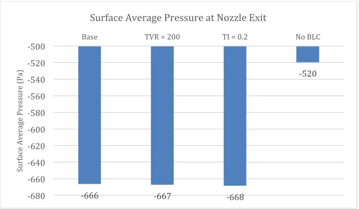
Figure 29. Surface Average Pressure at the Nozzle Exit. ... 43
Figure 30. Surface TKE at the Nozzle Exit. ... 44
Figure 31. Surface TVR at the Nozzle Exit. ... 44
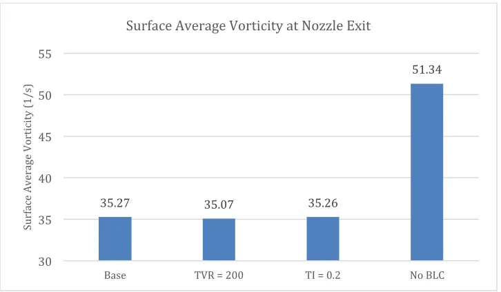
Figure 32. Surface Vorticity at the Nozzle Exit. ... 45
Figure 33. Base Simulation, Velocity Magnitude. ... 45
Figure 34. TVR = 200 Simulation, Velocity Magnitude. ... 46
Figure 36. No-BLC Simulation, Velocity Magnitude. ... 46
Figure 37. Base Simulation, Turbulent Kinetic Energy. ... 47
Figure 38. TVR = 200 Simulation, Turbulent Kinetic Energy. ... 47
Figure 39. TI= 0.2 Simulation, Turbulent Kinetic Energy. ... 47
Figure 40. No-BLC Simulation, Turbulent Kinetic Energy. ... 48
Figure 41. Base Simulation, Turbulent Viscosity Ratio. ... 48
Figure 42. TVR = 200 Simulation, Turbulent Viscosity Ratio. ... 48
Figure 43. TI= 0.2 Simulation, Turbulent Viscosity Ratio. ... 49
Figure 44. No BLC Simulation, Turbulent Viscosity Ratio. ... 49
Figure 45. Base Simulation, Vorticity Magnitude. ... 49
Figure 46. TVR = 200 Simulation, Vorticity Magnitude. ... 50
Figure 47. TI= 0.2 Simulation, Vorticity Magnitude. ... 50
Figure 48. No BLC Simulation, Vorticity Magnitude. ... 50
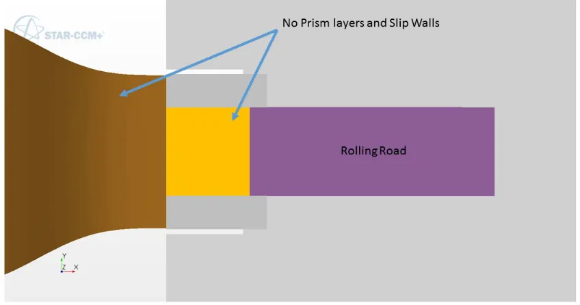
Figure 49. Modifications to WindShear simulation. ... 53
Figure 50. Velocity Magnitude Uniformity at Nozzle Exit. ... 53
Figure 51. Surface Average Velocity at the Nozzle Exit. ... 54
Figure 52. Surface Average TKE at Nozzle Exit. ... 54
Figure 53. Surface Average TVR at Nozzle Exit. ... 55
Figure 54. Surface Average Vorticity at Nozzle Exit. ... 55
Figure 57. Velocity Vectors for YZ Plane at X=0 with the Modified Simulation. ... 57
Figure 58. Velocity Magnitude at the YZ Plane at X=-7.5 meters (nozzle exit) with the Modified Simulation. ... 57
Figure 59. Surface Average Pressure at the Nozzle Exit. ... 58
Figure 60. Pressure at the YZ Plane at X=-7.5 Meters (nozzle exit) with the Base Simulation. ... 58
Figure 61. Pressure at the YZ Plane at X=-7.5 meters (Nozzle Exit) with the Modified Simulation. ... 59
Figure 62. Plan view of NASCAR vehicle used for simulation. ... 65
Figure 63. Side view of NASCAR vehicle used for simulation. ... 65
Figure 64. Front view of NASCAR vehicle used for simulation. ... 66
Figure 65. Bottom view of NASCAR vehicle used for simulation. ... 66
Figure 66. Rear view of NASCAR vehicle used for simulation. ... 67
Figure 67. Bottom view of the NASCAR vehicle with the splitter and radiator pan in red. ... 67
Figure 68. Bottom view of the NASCAR vehicle with the splitter in red and the radiator pan in blue. ... 68
Figure 69. Plan view of the generic NASCAR sedan in the WindShear wind tunnel. ... 71
Figure 70. Side view of the generic NASCAR sedan in the WindShear wind tunnel. .... 72
Figure 71. Mesh on the XZ pane at y = 0. ... 72
Figure 73. Detailed view of the mesh on the XZ pane at y = 0 showing the splitter and
radiator pan. ... 73
Figure 74. Velocity magnitude on the YZ plane 1 m upstream of the vehicle. ... 74
Figure 75. Coefficient of pressure on the XZ plane 1 m upstream of the vehicle. ... 74
Figure 76. TKE on the YZ plane 1 m upstream of the vehicle. ... 75
Figure 77. TVR on the YZ plane 1 m upstream of the vehicle. ... 75
Figure 78. Vorticity magnitude on the YZ plane 1 m upstream of the vehicle. ... 76
Figure 79. Velocity magnitude on the XZ plane at y = 0. ... 76
Figure 80. Velocity magnitude on the XZ plane at y = 0, showing the vehicle in detail. 77 Figure 81. Velocity magnitude on the XZ plane at y = 0, showing the splitter in detail. 77 Figure 82. Coefficient of pressure on the XZ plane at y = 0, showing the splitter in detail. ... 78
Figure 83. Coefficient of total pressure on the XZ plane at y = 0, showing the splitter in detail. ... 78
Figure 84. Coefficient of pressure on the underside of the vehicle. ... 79
Figure 85. Near-surface velocity vectors on the splitter and radiator pan. ... 79
Figure 86. Coefficient of pressure on the splitter and radiator pan. ... 80
Figure 87. Coefficient of skin friction on the splitter and radiator pan. ... 80
Figure 88. Contours of total pressure plotted on a XY plane at a height of 5 mm. ... 81
Figure 89. Plan view of the generic NASCAR sedan in a flow box. ... 83
Figure 90. Side view of the generic NASCAR sedan in a flow box. ... 84
Figure 92. Detailed view of the mesh on the XZ pane at y = 0, showing the vehicle. ... 85
Figure 93. Velocity magnitude on the YZ plane 1 m upstream of the vehicle. ... 85
Figure 94. Coefficient of pressure on the YZ plane 1 m upstream of the vehicle. ... 86
Figure 95. TKE on the YZ plane 1 m upstream of the vehicle. ... 86
Figure 96. TVR on the YZ plane 1 m upstream of the vehicle. ... 87
Figure 97. Vorticity magnitude on the YZ plane 1 m upstream of the vehicle. ... 87
Figure 98. Velocity magnitude on the XZ plane at y = 0. ... 88
Figure 99. Velocity magnitude on the XZ plane at y = 0, showing the vehicle in detail. 88 Figure 100. Velocity magnitude on the XZ plane at y = 0, showing the splitter in detail. ... 89
Figure 101. Coefficient of pressure on the XZ plane at y = 0, showing the splitter in detail. ... 89
Figure 102. Coefficient of total pressure on the XZ plane at y = 0, showing the splitter in detail. ... 90
Figure 103. Coefficient of pressure on the underside of the vehicle. ... 90
Figure 104. Near-surface velocity vectors on the splitter and radiator pan. ... 91
Figure 105. Coefficient of pressure on the splitter and radiator pan. ... 91
Figure 106. Coefficient of skin friction on the splitter and radiator pan. ... 92
Figure 107. Contours of total pressure plotted on a XY plane at a height of 5 mm. ... 92
Figure 108. Cp for the splitter and pan plotted vs X position for Y = 0. ... 93
Figure 109. Plan view of generic F1 vehicle used for simulation. ... 97
Figure 111. Front view of generic F1 vehicle used for simulation. ... 98
Figure 112. Bottom view of generic F1 vehicle used for simulation. ... 99
Figure 113. Rear view of generic F1 vehicle used for simulation. ... 99
Figure 114. Mesh of generic F1 in WindShear. ... 100
Figure 115. Mesh of generic F1 in WindShear. ... 100
Figure 116. Mesh of generic F1 in WindShear. ... 101
Figure 117. Mesh of generic F1 in WindShear YZ plane at X = 0. ... 101
Figure 118. Heat exchange placement in model. ... 102
Figure 119. Base, showing contours of velocity magnitude on the XZ plane at Y = 0. . 102
Figure 120. Base, showing contours of velocity magnitude with details of the vehicle. 103 Figure 121. Base, showing contours of velocity magnitude with details of the front wing. ... 103
Figure 122. Base, showing contours of velocity magnitude with details of the rear of the vehicle. ... 104
Figure 123. Base, showing contours of velocity magnitude on the XZ plane at Y = -0.4. ... 104
Figure 124. Base, showing contours of coefficient of total pressure on the XZ plane at Y = -0.4. ... 105
Figure 125. Figure 108: Base, showing contours of velocity magnitude at the nozzle exit. ... 105
Figure 127. Figure 110: Base, showing contours of turbulent viscosity ratio at the nozzle
exit. ... 106
Figure 128. Figure 111: Base, showing contours of vorticity magnitude at the nozzle exit. ... 107
Figure 129. TVR = 200; contours of velocity magnitude showing details of the vehicle. ... 107
Figure 130. TVR =200; contours of velocity magnitude showing details of the front wing. ... 108
Figure 131.Figure 114: TVR =200; contours of velocity magnitude showing details of the rear of the vehicle. ... 108
Figure 132. TVR = 200; contours of velocity magnitude on the XZ plane at Y = -0.4. 109 Figure 133. TVR = 200; contours of coefficient of total pressure on the XZ plane at Y = -0.4. ... 109
Figure 134. TVR = 200; contours of velocity magnitude at the nozzle exit. ... 110
Figure 135. TVR = 200; contours of turbulent kinetic energy at the nozzle exit. ... 110
Figure 136. TVR =200; contours of turbulent viscosity ratio at the nozzle exit. ... 111
Figure 137. Contours of vorticity magnitude at the nozzle exit. ... 111
Figure 138. TVR =200; contours of velocity magnitude showing details of the vehicle. ... 112
Figure 140. TI = 0.2; contours of velocity magnitude showing details of the rear of the
vehicle. ... 113
Figure 141. TI = 0.2; contours of velocity magnitude on the XZ plane at Y = -0.4. ... 113
Figure 142. TI = 0.2; contours of coefficient of total pressure on the XZ plane at Y = -0.4... 114
Figure 143. TI = 0.2; contours of velocity magnitude at the nozzle exit. ... 114
Figure 144. TI = 0.2; contours of turbulent kinetic energy at the nozzle exit. ... 115
Figure 145. TI = 0.2; contours of turbulent viscosity ratio at the nozzle exit. ... 115
Figure 146. TI = 0.2; contours of vorticity magnitude at the nozzle exit. ... 116
Figure 147. Surface-average TKE on the YZ plane at the nozzle exit. ... 116
Figure 148. Surface average TVR on the YZ plane at the nozzle exit. ... 117
Figure 149. % Change for lift-related metrics ... 118
Figure 150. Base flow box simulation with inlet positioned 12.5 m in front of the vehicle. ... 121
Figure 151. Inlet Base –6 m. ... 121
Figure 152. Inlet base +6 m. ... 122
Figure 153. Base flow box TKE on an YZ plane at X = -4.5. ... 122
Figure 154. Base flow box – 6 m, TKE on an YZ plane at X = -4.5. ... 123
Figure 155. Base flow box + 6 m, TKE on an YZ plane at X = -4.5. ... 123
Figure 156. Base flow box TVR on an YZ plane at X = -4.5. ... 124
Figure 157. Base flow box -6 m, TVR on an YZ plane at X = -4.5. ... 124
Figure 159. Surface average turbulent kinetic energy on an YZ plane at X = -4.5. ... 125 Figure 160. Surface average turbulent viscosity ratio on an YZ plane at X = -4.5. ... 126 Figure 161. Base; velocity magnitude on XZ plane at Y=0. ... 127 Figure 162. Base -6 m; velocity vectors on XZ plane at Y=0. ... 127 Figure 163. Base +6 m; velocity vectors on XZ plane at Y=0. ... 128 Figure 164. Base; velocity magnitude on XZ plane at Y=0. ... 128 Figure 165. Base -6 m; velocity vectors on XZ plane at Y=0. ... 129 Figure 166. Base +6 meters; velocity vectors on XZ plane at Y=0. ... 129 Figure 167. Base; coefficient of total pressure on XZ plane at Y=0. ... 130 Figure 168. Base -6 meters; coefficient of total pressure on XZ plane at Y=0. ... 130 Figure 169. Base +6 m; coefficient of total pressure on XZ plane at Y=0. ... 131 Figure 170. Inlet position VS Cl. ... 131
Figure 171. SA turbulence model; velocity magnitude on XZ plane at Y=0. ... 132 Figure 172. SA turbulence model; velocity magnitude on XZ plane at Y=0. ... 133 Figure 173. SA turbulence model; coefficient of total pressure on XZ plane at Y=0. .. 133 Figure 174. Bottom view of the NASCAR vehicle with the splitter and radiator pan in
red. ... 137 Figure 175. Bottom view of the NASCAR vehicle with the splitter in red and the
Figure 179. Ground clearance vs. coefficient of drag. ... 147 Figure 180. Cp VS Z position for flat plates. ... 148
Figure 181. Plate in computational domain. ... 149 Figure 182. Mesh on symmetry plane. ... 149 Figure 183. Mesh on symmetry plane, complete view. ... 150 Figure 184. Plan view of plate showing the mesh. ... 150 Figure 185. Front view of mesh, XY plane. ... 151 Figure 186. Front view of mesh, XY plane complete view. ... 151 Figure 187. Ground clearance is 0.0357% of cord. ... 152 Figure 188. Ground clearance is 0.0714% of cord. ... 152 Figure 189. Ground clearance is 1.7143% of cord. ... 153 Figure 190. Base size of 16. ... 153 Figure 191. Base size of 25.6. ... 154 Figure 192. Base size of 16. ... 154 Figure 193. Base size of 25.6. ... 155 Figure 194. Base size of 16. ... 155 Figure 195. Base size of 25.6. ... 156 Figure 196. Total number of cells in the mesh vs Cl. ... 156
Figure 197. Total number of cells in the mesh vs Cd. ... 157
Figure 201. Velocity magnitude with base size 25.6. ... 159 Figure 202. Comparison of turbulence models for Cl. ... 159
Figure 203. Comparison of turbulence models for Cd. ... 160
Figure 204. Velocity magnitude for the base turbulence model. ... 161 Figure 205. Velocity magnitude with k-ε. ... 161 Figure 206. Velocity magnitude with SA. ... 162 Figure 207. Velocity magnitude with RST. ... 162 Figure 208. Comparison of CFD simulation to the calculated Blasius. ... 163 Figure 209. Mesh for the low Re case. ... 163 Figure 210. Prism layers for the low Re case. ... 164 Figure 211. Contours of velocity magnitude for the low Re case. ... 164 Figure 212. Velocity vectors showing the boundary layer. ... 165 Figure 213. Side view of computational domain. ... 170 Figure 214. Plan view of computational domain. ... 171 Figure 215. Font view of computational domain... 171 Figure 216. Wing geometry. ... 172 Figure 217. Mesh on the symmetry plane. ... 172 Figure 218. Mesh on YZ plane at X = -2.35. ... 173 Figure 219. Detail of mesh showing prism layers on the ground plane and the wing. . 173 Figure 220. h/c vs. Cl for the F1 wing. ... 174
Figure 221. h/c for Cd for the F1 wing. ... 174
Figure 223. Contours of velocity magnitude for Y = 5 for h/c of 0.017. ... 175 Figure 224. Contours of velocity magnitude for Y = 5 for h/c of 0.083. ... 176 Figure 225. Contours of coefficient of total pressure for h/c of 0.033 (minimum Cl). .. 176
NOMENCLATURE
A platform or frontal area
b wing span
c chord
Cp coefficient of pressure, p/q
CLf front lift coefficient on the front wheels CLr rear lift coefficient on the rear wheels CL lift coefficient
D diameter
h ride height
hf front ride height; height of the projected floor at front axle centerline hr rear ride height; height of the projected floor at rear axle centerline
H height
l lift, positive indicates lift,
L length
p static pressure
q dynamic head, 1 2𝜌𝑈!!
Re Reynolds number based on either wing chord u,v,w streamwise, traverse, and spanwise velocity components
U freestream velocity
W width
x, y , z Cartesian coordinates, x positive downstream, y positive upwards
Greek Symbols
α incidence, positive for a nose down rotation ᶿ angle of diffuser or rotation
Glossary
CHAPTER 1. INTRODUCTION
A current focus in road vehicle production is aerodynamics development, the engineering of vehicles to minimize wind resistance while the vehicle is in motion. A primary objective in road vehicle aerodynamic development is to reduce drag, the friction between air and vehicle, which is a major determinant of the road load power required to move a vehicle. Drag can be reduced by adjusting the attitude of the vehicle and its proximity to the ground plane. One benefit of reducing aerodynamic drag is that it can significantly reduce fuel consumption, and thus, carbon emissions. In developed
countries, legislation is often used in efforts to reduce vehicles’ fossil fuel consumption and the associated costs of operation, including carbon emissions. The widespread drive to reduce carbon emissions from both heavy- and light-duty vehicles has made drag reduction the dominant factor in road vehicle aerodynamic development. After drag reduction, the second priority in vehicle aerodynamic development is aero-acoustic noise reduction, which is driven by consumers’ demand for quieter vehicles. Additional
development criteria for which vehicles must meet target performance objectives include lift control, cross-wind stability, visibility, cooling, and climate control.
1.1 Background
In many ways, ground vehicles’ aerodynamics are more complex than those of aircraft. Because a road vehicle has a bluff shape, it is difficult to discretize into sub-regions, and its flow field has large viscous regions of separated flow and a large wake. By contrast, aircraft are streamlined, and the flow field is generally dominated by inviscid flow; any viscous effects are limited to the boundary layer and a small wake, with the flow generally attached to the body.
Both road and motorsport vehicles operate in close ground proximity, and the effect of the ground proximity may never be ignored in aerodynamic development. Professional motorsport vehicles move at greater speed and are closer to the ground than production road vehicles, and they must meet sanction regulations and performance objectives that can be orders of magnitude greater than for road vehicles. In most top-level motorsports series, the clear objective of aerodynamics development is to maximize the lift-to-drag ratio (L/D). In some series, such as the top-level American sedan series controlled by the sanctioning body NASCAR, regulations strictly control the parts of the vehicle where aerodynamic development may occur. In these environments, drag
reduction at a given lift is somewhat less important, and the objective becomes to minimize lift for the regulations.
In both the original equipment manufacturer (OEM) and motorsport
dynamics (CFD). Each tool has its strengths and limitations, and no tool provides a complete picture of a vehicle’s aerodynamic performance. However, when all of the tools are used in conjunction and appropriately, they give the most well-defined definition possible of the aerodynamic performance envelope of a ground vehicle. This work used both wind tunnel and CFD simulation, which are both described below.
1.1.1 Wind Tunnel Simulations
The wind tunnel is the primary ground vehicle aerodynamic development tool for both motorsport and industry. In general, the validation of any vehicular aerodynamic simulation will likely be in a wind tunnel. Wind tunnels offer a laboratory-controlled environment to measure aerodynamic performance empirically. Empirical work in wind tunnels dominates ground vehicle aerodynamic development because of the nature of the vehicles’ bluff shapes. As the complexity of testing has increased over the decades, along with the demand to reduce development cycle time, the motorsports industry has been forced to move from the rental of aerospace wind tunnels to dedicated tunnels. The wind tunnels used for automotive aerodynamic development have evolved into highly
specialized facilities.
Despite their widespread use, wind tunnels can only simulate the conditions of the road, not reproduce them exactly. The flow field in an automotive wind tunnel is an extreme simplification of reality. The aerodynamic forces on the vehicle are a function of pressure and area:
For the aerodynamic forces to be accurate in a wind tunnel simulation, the pressure distribution must be accurate. Velocity and pressure are related. The Euler equation with gravity and viscous forces neglected is as follows:
𝑑𝑝 = −𝜌𝑉𝑑𝑉 (1)
Integrating from P1 to P2 along a streamline, the equation is as follows:
𝑝2−𝑝1 +𝜌 !!𝑉!!−!
!𝑉!
! = 0 (2)
or 𝑝1+!!𝜌𝑉!! =𝑝2+!
!𝜌𝑉!
! (3) Equation 3 is also known as Bernoulli’s equation.
Because the pressure at every point on the vehicle is proportional to the square of the local velocity, any errors in the velocity distribution have a significant impact on the test results.
significantly more difficult than in other types of wind tunnels and may lead to a loss of resolution.
Because of the ground proximity of road and motorsport vehicles, accurate results in wind tunnel simulations depend upon control of the boundary layer. A boundary layer forms when air flows along the side of the vehicle; as the air at the side of the vehicle adheres to the vehicle, its velocity is zero. Wind tunnels dedicated to ground vehicle testing are equipped with advanced boundary-layer control systems. In many cases, two boundary layer controls are used, a primary and a secondary control. For moving-ground-plane wind tunnels, the primary and secondary boundary layer suction removes the boundary layer immediately upstream of the model, allowing the remaining free stream to follow the belt. The belt moves at the free-stream velocity, so no ground boundary layer will develop. This approach, in combination with wheel rotation, provides the highest possible fidelity in automotive aerodynamic laboratory testing.
1.1.2 CFD Simulation
automotive industry to reduce the duration of product development cycles. In automotive development, CFD simulation is used for external aerodynamics, for internal flows, and at the component level. Most automotive flows are relatively low-speed, incompressible, and turbulent. These flow fields are generally unsteady or time-dependent, although in many cases, they can be successfully approximated as steady cases. The challenge with using CFD is to manage the tradeoff of the requirement for increased accuracy with processing time. CFD often struggles to produce the accuracy and the resolution of wind-tunnel testing. Resolution and solution time must be balanced against computational expense. Due to this limitation, CFD is often best used early in the design process to evaluate the potential of various concepts.
CFD is also used for visualization of the flow field. In the wind tunnel, flow field visualization is made possible by particle image velocimetry (PIV), a measurement technique that involves the use of a laser, seed particles, and camera(s). Although it is a valuable tool for understanding the flow field, and the data it provides may be used to validate a CFD simulation, the technique is often cumbersome and time-consuming to use. A properly validated CFD model may be a more flexible tool to visualize the flow field than using PIV with a wind-tunnel simulation. Indeed, one of the primary strengths of CFD is its visualization of the flow field. CFD provides a faster and more flexible method of flow visualization than PIV.
particularly influenced by the ground plane. This creates challenges for CFD, as the field under the vehicle must be modeled correctly to provide good correlation to empirical results from wind-tunnel simulations or over-the-road tests. At present, CFD is used in motorsports to augment empirical testing rather than replace it. Several unsuccessful attempts have been made to replace traditional wind-tunnel testing with CFD simulation. The most notable is the former Virgin Racing F1 team; their 2010 F1 car was designed and developed using CFD exclusively (38). This attempt to rely entirely on CFD for aerodynamic development failed, and the cars were not competitive. For the development of the 2012 car, the team moved to a more traditional wind-tunnel-based development program, augmented with CFD, and achieved significantly better performance. (39) For motorsports applications, the through-put of CFD often becomes a limiting factor. To obtain the required resolution, the model size becomes very large, and the solution time increases. During a wind tunnel test, it is common for two to three model changes to be achieved per hour. In CFD, it may take five to 10 times as long to complete the same work. In the fast-paced environment of motorsport aerodynamic development, speed relates directly to on-track performance, and CFD with the current limitations is neither fast nor accurate enough to replace empirical testing completely.
1.1.3 Boundary Layers, Turbulence, Lift, and Drag in Simulations
the no-slip condition at the wall and the free stream some distance away. The boundary layer is the portion of the flow field (adjacent to the wall that contains the velocity gradient) where the viscous effects are significant. The velocity gradient will be between zero (at the fluid wall interface) and the free stream velocity. Two classifications for boundary layers are laminar and turbulent. While a laminar boundary layer has a smooth, organized flow, a turbulent boundary layer is disorganized and contains eddies. Boundary layers grow with the length of the flow over the surface. A boundary layer flow can be characterized as either laminar or turbulent based on the ratio of inertial forces to viscous forces, or the Reynolds Number (Re). All interesting automotive simulations are in the turbulent flow regime.
Any study of vehicle aerodynamics must make use of turbulence models. Turbulence occurs when inertial forces are larger than the viscous forces, and it is characterized by chaotic flow. A turbulent flow is made up of eddies of different sizes. Turbulence models provide a means of simulating the effects of turbulent fluctuations from the mean flow state. Energy is taken from the mean flow by the largest eddies, which are unstable and eventually break up into smaller eddies. Energy is passed down from the macro scale of the large-scale eddies to smaller-scale eddies. This transfer of energy continues until the length-scale of the motion is sufficiently small that the viscosity of the fluid can effectively dissipate the kinetic energy at the micro scale. This is known as the energy cascade. Turbulence has significant impacts on vehicle
vehicles, turbulence can re-energize the boundary layer, and in some cases it can delay separation, improving aerodynamic performance. Accurate modeling of turbulence is critical to the proper calculation of lift and drag. All turbulence models are an
approximation, and in any given automotive simulation, it is not likely that one
turbulence model will provide a good fit for the entire flow field. As a result, predicting where a flow field separates from a surface can be a significant challenge.
To approximate the boundary layer over the lower portion of a vehicle’s splitter, it is possible to use a simplified two-dimensional solution for a laminar boundary layer over a semi-infinite flat plate. Paul Richard Heinrich Blasius (1908) was the first to use this simplified, two-dimensional alternative to complex differential equations. The complex relationships among the velocity, pressure, temperature, and density of a moving fluid are more fully described by the Navier-Stokes equations.
Any time- and space-dependent flow variable ∅(𝑥,𝑡) is decomposed, by
averaging or filtering, into a quantity that can be resolved ∅(𝑥,𝑡) and a component that cannot be resolved ∅(𝑥,𝑡)!. The effect of the unresolved flow structures on the resolved
ones is modeled as a force. For a Reynolds Averaged Naiver-Stokes (RANS) model, this would be the Reynolds Stress. The energy on the unresolved portion of the flow field is extremely significant and can exceed 30% of the flow field’s total energy.
Kolmogorov length scale = 𝑣! 𝜀 ! !
≈0.1𝑚𝑚
If four cells are used in each direction to resolve an eddy, 10e16 cells would be needed in a 10m x 10m x 20m wind tunnel. There are more unknowns than there are equations, so the Naiver-Stokes equations cannot be closed. A turbulence model must be used to close them. With up to 30% of the energy in the flow field being modeled, the method of closure becomes critical to balancing computational expense and accuracy.
All of the results reported in this work use RANS, where the turbulence is fully modeled. The base model used is the shear stress transport (SST) k-Omega two equation [AIAA Journal, Vol. 32, No. 8, August 1994, pp. 1598–1605]. For comparison, specific cases are presented with other turbulence models, including Spalart-Allmaras, k-Epsilon two equation, and the Reynolds Stress Transport seven equation.
The SST k-Omega model is a two-equation model that blends the k-Omega near-wall model with a transformed k-Epsilon model in the bulk flow. This model performs well in adverse pressure gradients, but it may over-predict separation. Proper meshing is critical for the performance of this model. In motorsports CFD modeling of critical aerodynamic components, it is necessary to resolve the viscous sub-layer with appropriate prism layers. As a result, the y+ values will be < 1.
1.2 Purpose and Scope
less accurate as the x position is increased along the length of the vehicle model. The rear of the vehicle is less accurate than the front. Boundary layers grow with length, and the interaction of vortices increases the difficulty of the simulation. The upper surface of the vehicle is more accurate than the lower due to the turbulent nature of the flow field under the vehicle. CFD simulations of bluff bodies are difficult due to the large-scale separation of the flow and the highly turbulent wake. Adding ground proximity to the simulation of a bluff body adds another layer of complexity. This work adds to the knowledge of ground vehicle simulation by investigating techniques to simulate ground vehicles. The scope encompasses ground vehicle simulations in general but also motorsports ground vehicles specifically.
1.3 Procedure
After this first round of simulations, several more tests were run. A NASCAR sedan was tested in the Windshear tunnel model and in a standard flow box, and the results were compared to those from the simulation of the wind tunnel itself. Next, a generic F1 model was tested in the Windshear tunnel model; a simulation was run with changes made to the boundary-layer control. Then, another simulation was run with changes to the inlet turbulence intensity and turbulent viscosity ration conditions. The generic F1 car was then simulated in a flow box. Simulations were then run with the F1 car in the flow box, changing the inlet position, and with changes to the inlet turbulence intensity and turbulent viscosity ration conditions.
In order to understand how ground proximity affects the performance of a flat plate, a series of 23 simulations were performed. A plate was simulated with the following ground clearances h/c=:
• 0.0357 • 0.0536 • 0.0714 • 0.1071 • 0.1429 • 0.2143 • 0.4286 • 0.8571 • 1.7143
The plate was then fixed at a ground clearance of h/c = 0.1071, and the following turbulence models were run:
• Base Segregated KW SST Rans • Modified KW A1 =1
The plate was then run at a fixed ground clearance of h/c = 0.1071, with varying mesh densities, to look at mesh dependency.
• Base of 12.8 mm • Base of 16 mm • Base of 19.2 mm • Base of 22.4 mm • Base of 25.6 mm
A generic multi-element F1-style front wing was simulated with the following ground clearances of h/c=:
• 0.017 • 0.033 • 0.050 • 0.067 • 0.083 • 0.167 • 0.25 • 0.33 • 0.833 • 1.667
The generic multi-element F1-style front wing was then fixed at a ground clearance of h/c = 0.067, and different turbulence models were run:
1. Base Segregated KW SST Rans 2. Modified Segregated KW SST Rans 3. Segregated K Omega
4. Segregated SA
moving belt ground plan, a simulation of the wind tunnel was first completed. To validate the model, the boundary layer profile of the wind tunnel CFD simulation was compared to empirical measurements made in the wind tunnel’s test section. The results of the comparison showed that the simulation provides excellent correlation to the empirical measurements made in the wind tunnel. CAD models for both a NASCAR-style competition vehicle and an open-wheel F1-style vehicle were created and placed in the CAD model of the wind tunnel. A CFD simulation of each vehicle in the wind tunnel was performed. The coefficient of lift front (Clf), coefficient of lift rear (Clr), coefficient of lift total (Clt), and coefficient of drag (Cd) were calculated for each vehicle in the wind tunnel. The lift, drag, and balance all had less than 10% error when compared with results from the NASCAR-style vehicle. No empirical results were available for the generic open-wheel F1 vehicle model, making a direct validation comparison impossible.
To understand the effect of the wind tunnel model on the overall simulation, the vehicles were used in a simulation without the wind tunnel in a plane rectangular
computational domain. Modifications were performed on the inlet conditions to the flow box to understand the impact on the vehicle simulations. The study showed that good results can be obtained with a simple flow box. In many cases, the wind tunnel model is not necessary, and its complexity and computational expense can be eliminated. For the most exact comparisons, though, the wind tunnel model should be included.
study the effect of the proximity of the ground on this key aerodynamic device, a flat rectangular plate with dimension similar to the splitter was used. Flow over this flat plate was studied at a height above the ground plane from a height to cord ratio (h/c) of 0.0375 to 1.71. The effect of several turbulence models and simulation variables on the flow field were then studied. Finally, a laminar flow simulation of the flat plate was
CHAPTER 2. Wind Tunnel Simulation
2.1 Introduction and Literature Review
Wind tunnels are widely used for empirical research in ground vehicle
aerodynamics. In the development of vehicles for both motorsport and industry, the wind tunnel offers a laboratory-controlled environment to measure vehicles’ aerodynamic performance. However, wind tunnels offer only a simplified simulation of real road conditions, and the flow field in an automotive wind tunnel needs to be carefully
controlled to achieve accurate results. Particularly crucial is the control of the layer of the flow field in close proximity to walls, referred to as the boundary layer. The boundary layer control near the ground and in close proximity to the bottom of the vehicle is most critical. (1)(2)(4)
boundary layer flow as either laminar or turbulent is based on the ratio of inertial forces to viscous forces, which is the Reynolds Number. Turbulent flows are of great interest in automotive simulations because automotive bodies are primarily bluff with substantial regions of separated flow and large wakes. These flows have great implications for drag and lift, and thus for aerodynamic design. Automotive simulations differ from aircraft simulations in that aircraft are primarily streamlined, with small wakes and limited or no separated flow. (1)(2)
A wind tunnel is itself a simulation. In a wind tunnel, the relative motion of the road, ground plane, vehicle, and air are reversed. In the wind tunnel, the vehicle remains stationary while the air moves. Over the road, the vehicle moves through the air while the road is stationary. The air nearest the ground remains stationary. Over the road, the wheels rotate, which greatly affects the flow field downstream of the wheels and the pressures in the wheel housings. Accurate results in wind tunnel simulations for both road and motorsport vehicles depend upon control of the ground boundary layer, and on simulation of the wheel wakes. This is due to the close ground proximity of these
vehicles. If the boundary layer is not controlled, then it may grow in height to exceed the lower extremities of the vehicle. The stagnation point for passenger cars is generally less than 500 mm above the ground. For motorsports vehicles, this can be less than 100 mm. For turbulent flows over a flat plate, the thickness or height of the boundary layer δ may be approximated:
𝛿 ≈0.382𝑥
𝑅𝑒!!.!
Rex is the Reynolds number at the x location
X = the distance downstream from the start of the boundary layer
For a flow at 50 m/s in a wind tunnel with no boundary layer control where the vehicle is 10 meters downstream from the start of the test section δ≈ 116 mm. In the case of a motorsport vehicle that has a splitter or wing with a ground clearance of 10 mm, the boundary layer in this example would envelope a key aerodynamic device. This is of great concern in motorsport applications, as these vehicles routinely operate at ground clearances of 10 mm. In motorsport applications, in order to provide the necessary boundary layer control, wind tunnel tests are done in a wind tunnel with a moving belt floor and with a vehicle whose wheels rotate. Unfortunately, in this type of wind tunnel, it is very difficult to measure forces, potentially leading to a loss of resolution. For a wind tunnel simulation to model aerodynamic forces accurately, the pressure distribution must be precisely accounted for. Pressure is related to velocity, in that the pressure at every point on the vehicle is proportional to the square of the local velocity. Even a minor error in the velocity distribution can have a significant impact on the test results. Therefore, for both the wind tunnel and a CFD simulation, achieving a near-flat velocity gradient upstream of the vehicle is desired.
question, we performed 5 simulations using models of the WindShear wind tunnel. First, we simulated the WindShear wind tunnel geometry with no boundary layer control but with the rolling road. This simulation shows the growth of the uncontrolled boundary layer. Next, the WindShear wind tunnel was simulated with a fully modeled primary and secondary boundary layer control and a moving ground plane. The results of this
simulation were compared with empirical measurements from the WindShear wind tunnel. Next, we tested two changes to the turbulence conditions at the inlet to the computational domain, as well as their effect at the inlet to the test section. Finally, a modification to the boundary conditions and mesh strategy was used to see whether a similar inlet condition could be created without the expense of modeling the boundary layer control system. (3) (4) (5) (6)
2.2 Wind Tunnel Simulations
As previously stated, empirical results for the measurement of ground vehicle aerodynamics are most often achieved in a wind tunnel. The correlation of CFD
calculations is therefore usually correlated to wind tunnel measurements. Although wind tunnels are designed to limit their influence on the model being tested, the influence can be significant, especially for near-ground testing. (8) The purpose of these simulations is to gain an understanding of the best method to simulate a full-scale wind tunnel. The questions to be answered are:
• Can the primary and secondary boundary layer control systems be simulated accurately?
• How do changes in the turbulence conditions at the inlet of the computational domain affect the inlet to the test section?
• Is there a less computationally expensive method to achieve an acceptable test section velocity gradient than by modeling the details of the primary and secondary boundary layer control system?
2.2.1 The CAD Models and Geometry Used for the Simulation
A CFD simulation of the WindShear wind tunnel was created. The CAD surfaces were provided by WindShear Inc., of Concord, North Carolina. A check of key
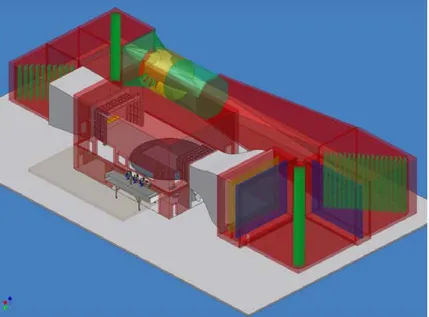
dimensions in the test section verified the accuracy of the supplied geometry. Image 1 shows the plan view of the WindShear wind tunnel. Image 2 shows a rendering of the wind tunnel’s key components. The computational domain of the WindShear CFD model includes the following:
• Contraction • Test section • Collector • Diffuser
Figure 2. Rendering of the wind tunnel's key components. (8)
The fan corners’ turning vanes were not modeled due the computational expense. A straight section upstream of the contraction was added to provide additional volume to organize and develop the inlet flow field. The velocity inlet to the computational domain was placed 15 meters upstream of the contraction. An additional 15-meter straight section was added downstream of the high-speed diffuser to remove any influence that the
model and the symmetry plane model. Figure 6 highlights the 15-meter straight sections added to the domain.
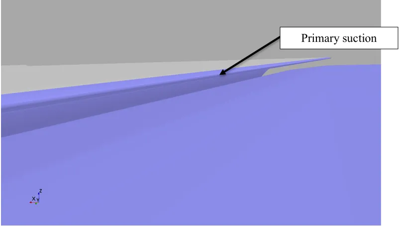
The boundary layer control system was modeled in fine detail. Figure 7 shows the primary and secondary boundary control systems in the model. Figure 8 shows the details of the primary boundary layer control system. Figure 9 shows the actual primary
boundary layer scoop at the WindShear wind tunnel. Figure 10 shows the secondary boundary layer control system in the model. Figure 11 shows the actual secondary boundary layer system.
Figure 4. Computational Domain Symmetry Plane Model, top view.
Figure 6. Added geometry.
Figure 8. Primary Boundary Layer Control System model.
Figure 9. Actual Primary Boundary Layer Scoop. (8)
Figure 10. Secondary Boundary Layer Control System model with tangential suction slots.
2.2.2 The Mesh for the Wind Tunnel Simulations
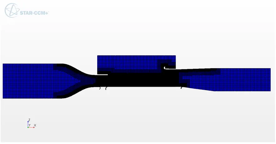
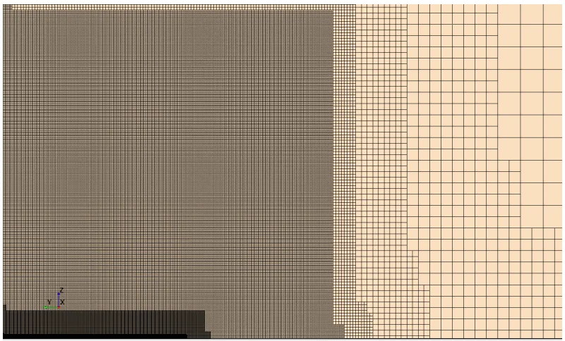
Mesh convergence was not possible with the computational resources available for this work. A traditional strategy was used, moving from a coarse mesh far from the area of interest to a fine mesh in the proximity of the area of interest. A quadrahedral trimmer mesh aligned with global coordinate system was used to mesh the WindShear model. This type of mesh tends to be more efficient as the grid lines are aligned with the bulk flow field. Prism layers were used on wall boundaries as an efficient way to model the near wall region. Prism layers allow high aspect-ratio cells to be placed adjacent to the wall without incurring excessive stream-wise resolution, which is not the case with other cell types. Prism layers reduce numerical diffusion near the wall by forcing cells connecting the prism to the bulk mesh to be aligned with the flow. Volume controls are generally simple geometric sub-regions inside the computational domain, such as boxes, cylinders, cones or spheres, typically created in CAD, where the volume mesh has specific settings that are different than the bulk mesh. In these simulations, volume refinements were used to increase mesh resolution in the boundary-layer control systems and test section.
The mesh in the test section near the rolling road was highly refined. The default settings for overall computational domain included a base size of 25 mm, with a
inlet and outlet walls. For these less critical surfaces, a large target size of 200 mm was used to reduce the overall size of the volume mess. The floor of the test section was meshed with a target size of 100 mm. No prism layers were used on the symmetry plane (for ½ model), or on inlet and outlet surfaces. The rolling road surface was the area of interest in this model and had special surface controls applied. The target size was reduced to 1.56 mm. The prism layer near-wall thickness was set to 0.01 mm, with a total prism layer thickness of 4.0 mm. A volume control was used in close proximity of the rolling road, where the size of the quadratic trimmer cells were set to 6.25 mm. A volume control was used for the region where the vehicle would be placed above the rolling road. The quadratic trimmer cells were set to 12.5 mm in this region. The effect of the volume controls can be seen in Figures 12 to 15.
Figure 12. WindShear simulation volume mesh X-Z plane.
Figure 14. WindShear simulation volume mesh Y-Z plane.
2.2.3 Physics Settings for the Wind Tunnel Simulations The WindShear models used the following physics settings: • Coupled Flow
• Constant Density Air, 1.1745 kg/m3
• RANS with SST (Menter) K-Omega Turbulence model
o a1 = 1
o Realizability Coefficient = 1.2 • All y+ Wall Treatment
The coupled flow model solves the conservation equations for mass, momentum, and energy simultaneously using a pseudo-time-marching approach. The coupled solver’s CPU time scales linearly with cell count, and is therefore less computationally expensive. In addition, the convergence rate does not deteriorate as the mesh is refined. The
disadvantage of the coupled solver is that it can be more difficult to achieve convergence if the mesh is less refined. (9) A constant density model was used for these cases as the average Mach number is << 0.3, and the peak Mach number is < 0.3; therefore, density affects are minimal. A two-equation eddy-viscosity turbulence model was chosen for these simulations. The two-equation k-ω model uses the turbulent kinetic energy (k) and turbulence-specific dissipation rate (ω) to define the turbulent eddy viscosity. This model shows improvement over the k-ε model in the prediction of flow separation, with both favorable and adverse pressure gradients. The k-ω performs well where the very near-wall physics modeling is of prime importance. (9) A near-wall treatment is a set of assumption for modeling the near-wall for the turbulence model. (10)
y+ is a non-dimensional wall distance for a flow bounded by a wall. 𝑦! ≡ 𝑢
𝑢∗≡ 𝜏! 𝜌
𝜏! =𝜇 !"!"
y = the distance from the wall to the cell centroid
ν = kinematic viscosity
Figure 16 shows the regions of applicability of the y+ wall treatments. The low y+ wall treatment assumes the viscous sublayer is well resolved by the mesh and is used when y+ < 1. High y+ wall treatment is the classic wall function approach first published by von Karmen (11), where wall shear stress, turbulent production, and turbulent
dissipation are all derived from equilibrium turbulent boundary layer theory. It is assumed that the near-wall cell lies within the logarithmic region of the boundary layer; therefore, the centroid of the cell attached to the wall should have y+ > 30.
The all-y+ wall treatment is an additional hybrid wall treatment that attempts to combine the high y+ wall treatment for coarse meshes and the low y+ wall treatment for fine meshes. It is designed to give results similar to the low y+ treatment as Y+
Figure 16. The regions of applicability of the y+ wall treatments.
The value for the turbulence quantity is calculated: Tq = gTq Low + (1-g)TqHigh where g is: g = exp(-Rey/11) where Rey is:
𝑅𝑒! = 𝑘𝑦 𝜈
y = the distance from the wall to the cell centroid
ν = kinematic viscosity
Figure 17. y+ values for the rolling road
2.2.4 Boundary Settings for the Wind Tunnel Simulations
The wind tunnel inlet was specified as a velocity inlet boundary with an 8.333334 m/s inlet velocity, with the direction normal to the boundary. With a contraction ratio of 6:1, a 50 m/s velocity was provided at the inlet to the test section. The turbulence
2.2.5 Wind Tunnel Base Simulations
To establish the base model, we first performed a simulation of the WindShear wind tunnel itself. We conducted the simulation both with and without the boundary-layer control system to show the significant effect of the boundary-control systems on the boundary layer in the wind tunnel test section. Figure 18 shows velocity vectors for the WindShear tunnel model without the boundary-layer control system, and Figure 19 shows velocity vectors for the WindShear tunnel model with the boundary-layer control system. The rolling road speed was set to 50 m/sec to match the nominal free stream near the ground in the test section. The outlet to the computational domain was set to a
pressure outlet, with the pressure set to 0.0 Pa gauge.
Figure 19. Velocity vectors for the WindShear tunnel model with the boundary-layer control system.
height above the ground plane is unacceptable for ground vehicle simulations. Figures 23 and 24 show velocity vectors in the YZ plane at the center of the rolling road without boundary-layer control and with, respectively. A comparison of these figures highlights the high degree of variance in the velocity field without the boundary-layer control despite the fact that the ground is moving at the free stream. It is evident that some form of boundary-layer control modeling is required for simulating ground vehicles in near-ground proximity.
Figure 20. U(x)/U(∞) VS. Z height (mm). 0 50 100 150 200 250
0 0.1 0.2 0.3 0.4 0.5 0.6 0.7 0.8 0.9 1
H ei gh t Ab ov e G ro un d Pl an e (mm) U(x)/U(∞)
Boundary Layer ProKile 2.5 m upsteam of Vehcile Center on center (SAE J2881)
With BLC (Base Model)
Figure 21. Turbulent Kinetic Energy for the WindShear tunnel model without the boundary-layer control system.
Figure 22. Turbulent Kinetic Energy for the WindShear tunnel model with the boundary-layer control system.
Figure 24. Velocity vectors for YZ plane at X=0 with the boundary-layer control system.
2.3 Comparison of the CD Model with Full-Modeled Boundary-Layer Control to Measured Data
Figure 25. Measurement of the velocity profile in the WindShear wind tunnel. (12) 0 5 10 15 20 25 30 35 40 45 50
0 0.2 0.4 0.6 0.8 1
H ei gh t Ab ov e G ro un d Pl an e (mm) U(x)/U(∞)
Boundary Layer ProKile 2.5 m upsteam of Vehcile Center (SAE J2881)
With BLC (Base Model)
2.4 Inlet Conditions
Turbulence conditions in front of the test object in the wind tunnel affect the lift and drag performance of the object being tested. Two changes to the computational domain’s inlet turbulence specifications were made, and their effects at the test section inlet were evaluated. Turbulence intensity was changed from 0.01 to 0.2, and
independently, the turbulence viscosity ratio was changed from 10 to 200. An YZ plane was created at the location X = -7.5 meters, which corresponds to the exit of the nozzle. Surface average values were measured across the tunnel at this location.
2.4.1 Results
Figures 27 to 36 compare velocity uniformity, surface average velocity, pressure, turbulent kinetic energy, turbulent viscosity, and vorticity respectively, for the base case, the no-boundary-layer control system case, and the two cases where inlet turbulence conditions were changed. Figures 33 through 36 show velocity magnitude on the YZ plane at X = -7.5 meters for the base model, TVR = 200, TI = 0.2 and the no-BLC simulations, respectively. Figures 37 through 40 show turbulent kinetic energy for the same location for the base model, TR = 200, TI = 0.2 and the no-BLC simulations, respectively. Figures 41 through 44 show turbulent viscosity ratio for the same location for the group of simulations. Figures 45 through 48 show vorticity magnitude on the YZ plane at X = -7.5 meters for the group of simulations.
viscosity ratio to 200 had the second-largest effect on the flow field. Changing the TVR value can be an effective way of tuning a wind tunnel simulation to match measured Cl and Cd values for ground vehicle simulations. Figure 42 shows the significant increase in TVR at the nozzle exit when compared to the other simulations. This may not be
surprising since the TVR was increased 1900% at the inlet to the computational domain. This showed a 214% increase in surface-averaged TVR at the nozzle exit. The 1900% increase in turbulence intensity at the inlet to the computational domain had no
measureable effect on the surface-averaged metrics or observable changes on the YZ plane at X = -7.5 meters. This inlet change is not effective as a tuning aid to wind tunnel simulations.
Figure 27. Velocity Magnitude Uniformity at the Nozzle Exit.
0.9914 0.9914 0.9914
0.9889 0.988 0.990 0.992 0.994 0.996 0.998 1.000
Base TVR = 200 TI = 0.2 No BLC
V el oc it y M ag ni tu de U ni fo rmi ty
Figure 28. Surface Average Velocity at the Nozzle Exit.
Figure 29. Surface Average Pressure at the Nozzle Exit.
48.94 48.95 48.91
51.34 48.5 49.0 49.5 50.0 50.5 51.0 51.5
Base TVR = 200 TI = 0.2 No BLC
Su rf ac e Av er ag e V el oc it y M ag ni tu de ( m/ s)
Surface Average Velocity Magnitude at Nozzle Exit
-666 -667 -668
-520 -680 -660 -640 -620 -600 -580 -560 -540 -520
-500 Base TVR = 200 TI = 0.2 No BLC
Su rf ac e Av er ag e Pr es su re ( Pa )
Figure 30. Surface TKE at the Nozzle Exit.
Figure 31. Surface TVR at the Nozzle Exit.
0.450 0.536 0.449 0.712 0.4 0.5 0.5 0.6 0.6 0.7 0.7 0.8
Base TVR = 200 TI = 0.2 No BLC
Su rf ac e Av er ag e T K E J/ kg
Surface Average TKE at Nozzle Exit
129
405
125 128
100 150 200 250 300 350 400
Base TVR = 200 TI = 0.2 No BLC
Su rf ac e Av er ag e T V R
Figure 32. Surface Vorticity at the Nozzle Exit.
Figure 33. Base Simulation, Velocity Magnitude.
35.27 35.07 35.26
51.34 30 35 40 45 50 55
Base TVR = 200 TI = 0.2 No BLC
Su rf ac e Av er ag e V or ti ci ty ( 1/ s)
Figure 34. TVR = 200 Simulation, Velocity Magnitude.
Figure 37. Base Simulation, Turbulent Kinetic Energy.
Figure 38. TVR = 200 Simulation, Turbulent Kinetic Energy.
Figure 40. No-BLC Simulation, Turbulent Kinetic Energy.
Figure 43. TI= 0.2 Simulation, Turbulent Viscosity Ratio.
Figure 44. No BLC Simulation, Turbulent Viscosity Ratio.
Figure 46. TVR = 200 Simulation, Vorticity Magnitude.
2.4.2 Emulating the Effect of the Boundary-Layer Control System without Direct Modeling
simulation and the base simulation. In this Figure, the overshoot of the target velocity can be seen as some of the data points exceed one. In addition, the floor velocity is
mismatched to the freestream average. A correction—or better, an iterative, closed-loop control to match the floor velocity to the free-stream average—would provide an
excellent velocity profile. Figure 56 shows velocity vectors for the WindShear tunnel model with the modifications. Figure 56 may be compared directly with the base
simulation in Figure 19. Figure 56 shows the removal of the BLC system. The bulk flow is very similar in magnitude and direction to the base simulation. Figures 57 and 58 may be compared directly with Figures 24 and 33, respectively. A comparison of these images to the base simulation shows qualitatively what the measured values show, that the modified simulation has greater uniformity in velocity magnitude than the base simulation.
Figure 49. Modifications to WindShear simulation.
Figure 50. Velocity Magnitude Uniformity at Nozzle Exit.
0.9914 0.9928 0.9889 0.988 0.990 0.992 0.994 0.996 0.998 1.000
Base Mod Mesh No BLC
V el oc it y M ag ni tu de U ni fo rmi ty
Figure 51. Surface Average Velocity at the Nozzle Exit.
Figure 52. Surface Average TKE at Nozzle Exit.
48.94 49.26 51.34 48.5 49.0 49.5 50.0 50.5 51.0 51.5
Base Mod Mesh No BLC
Su rf ac e Av er ag e V el oc it y M ag ni tu de (m/ s)
Surface Average Velocity Magnitude at Nozzle Exit
0.450 0.451
0.712 0.4 0.5 0.5 0.6 0.6 0.7 0.7 0.8
Base Mod Mesh No BLC
Su rf ac e Av er ag e T K E J/ kg
Figure 53. Surface Average TVR at Nozzle Exit.
Figure 54. Surface Average Vorticity at Nozzle Exit.
129 130 128
100 150 200 250 300 350 400
Base Mod Mesh No BLC
Su rf ac e Av er ag e T V R
Surface Average TVR at Nozzle Exit
35.27 35.57
51.34 30 35 40 45 50 55
Base Mod Mesh No BLC
Su rf ac e Av er ag e V or ti ci ty ( 1/ s)
Figure 55. U(x)/U (∞) VS. Z height (mm) Showing the Base and Modified Simulations.
Figure 56. Velocity Vectors for the WindShear Tunnel Model with the Modifications. 0 50 100 150 200 250
0.5 0.6 0.7 0.8 0.9 1
H ei gh t Ab ov e G ro un d Pl an e (mm) U(x)/U(∞)
Boundary Layer ProKile 2.5 m upsteam of
Vehcile Center (SAE J2881)
Base