Standard Error Computations for Uncertainty
Quantification in Inverse Problems: Asymptotic
Theory vs. Bootstrapping
H. T. Banks, Kathleen Holm and Danielle Robbins
Center for Research in Scientific Computation
and
Center for Quantitative Sciences in Biomedicine
North Carolina State University
Raleigh, NC 27695-8212
August 2, 2009
Abstract
We computationally investigate two approaches for uncertainty quantification in inverse problems for nonlinear parameter dependent dynamical systems. We compare the bootstrapping and asymptotic theory approaches for problems involv-ing data with several noise forms and levels. We consider both constant variance absolute error data and relative error which produces non-constant variance data in our parameter estimation formulations. We compare and contrast parameter estimates, standard errors, confidence intervals, and computational times for both bootstrapping and asymptotic theory methods.
1
Introduction
One of the more ubiquitous problems in all of science and engineering is the inverse prob-lem for estimation of parameters from longitudinal observations of system responses. This is usually formulated in terms of a parameter dependent dynamical system (or-dinary, partial, delay differential or integral equation (see [1, 2, 3, 7, 8, 10, 18, 19, 20, 21, 29, 30] and the references therein) for which observations of solutions (or certain components of the solutions) are to be used to estimate some unknown parameters 𝑞. In particular the general inverse problem for nonlinear parameter dependent ordinary differential equations is formulated in terms of a system
𝑑𝑥
𝑑𝑡(𝑡) =ℱ(𝑡, 𝑥(𝑡), 𝑞)
𝑥(0) =𝑥0,
(1)
with observations
𝑦𝑗 =𝑓(𝑡𝑗, 𝜃) =𝒞𝑥(𝑡𝑗;𝜃), 𝑗 = 1, . . . , 𝑛, (2)
where the solutions𝑥(𝑡;𝜃) in general depend on unknowns𝑞 and the (possibly unknown) initial conditions 𝑥0 so that 𝜃 = (𝑞, 𝑥0). In addition to computing estimates ˆ𝜃 for the unknown parameters using observations {𝑦𝑗}, it is widely accepted that quantifying
the uncertainty in these parameter estimates is equally important. A standard method [3, 4, 6, 8, 14, 16, 25] to do this involves computation of standard errors (SE) to be used
inconfidence intervals(CI) for the parameter estimates. Discussions of the fundamental
ideas and methods that are accessible to non-statisticians can be found in [3, 8].
In this note we investigate computationally and compare the bootstrapping approach and the asymptotic theory approach to computing parameter standard errors corre-sponding to data with various noise levels 𝑁𝑙. We consider both absolute error (with constant variance) measurement data and relative error (and hence non-constant vari-ance) measurement data sets in obtaining parameter estimates. Both types of errors are found widely in measurement procedures used in science and engineering investigations. We compare and contrast parameter estimates, standard errors, confidence intervals, and computational times for both bootstrapping and asymptotic theory approaches. Our goal is to investigate and illustrate some possible advantages/disadvantages of each approach in treating problems for nonlinear dynamical systems. We discuss these in the context of a simple example for which an analytical solution is available to provide readily obvious distinct qualitative behaviors. We chose this example because its solu-tions have many features found in those of much more complicated models: regions of rapid change as well as a region near an equilibrium with very little change and different regions of relative insensitivity of solutions to different parameters.
logistic model (also called the Verhulst-Pearl growth model) given by
𝑑𝑥(𝑡)
𝑑𝑡 =𝑟𝑥(𝑡)
(
1− 𝑥(𝑡)
𝐾
)
, 𝑥(0) =𝑥0.
Here𝐾 is thecarrying capacity as well as the asymptote value for solutions (as𝑡→ ∞)
0 5 10 15 20 25 0
2 4 6 8 10 12 14 16 18
Time
True Model
True Solution vs. Time
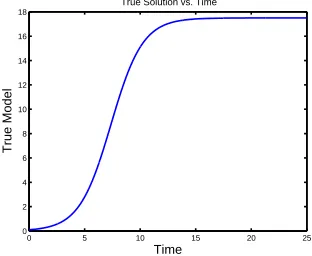
Figure 1: Logistic curve with 𝐾 = 17.5,𝑟 =.7 and 𝑥0 =.1.
and 𝑟 is the intrinsic growth rate.
The solution is given for 𝜃 = (𝐾, 𝑟, 𝑥0) by
𝑥(𝑡) = 𝑓(𝑡, 𝜃) = 𝐾 1 + (𝐾
𝑥0 −1)𝑒
−𝑟𝑡,
and is plotted in Figure 1 for 𝐾 = 17.5, 𝑟=.7 and 𝑥0 = 1 and 0≤𝑡≤25.
There is a substantial statistical literature (see [12, 15, 16, 23] and their references) on the use of the bootstrap in nonlinear regression problems while Chapter 12 of [25] con-tains a readable presentation for the corresponding use of asymptotic theory estimates in regression. As will be discussed in illustrative examples below, for quantifying uncer-tainty in parameter estimates the asymptotic theory is always faster computationally than bootstrapping. This unfortunately is the only definitive comparison that can be made. One of the two methods may be favored over the other dependent on the type of observational data set used. For constant variance data there appears to be little advantage for either method. Bootstrapping may be more reasonable for estimating the standard error in the cases of nonlinear systems so complex as to prohibit computation of the sensitivities needed for asymptotic theory errors. However, if computation time is already a concern and sensitivities can be computed, then asymptotic theory may prove advantageous.
least squares; in this case the asymptotic theory error estimates and the bootstrapping error estimates may be comparable. In some situations (when local variation in the data is high), the standard errors for bootstrapping are likely to be larger (due to a positive additive corrective term) but also more accurate than those of the asymptotic theory,. Otherwise as we shall illustrate, there will be insignificant correction in the bootstrap’s estimate of standard error over that of the asymptotic theory. Hence, the choice between bootstrapping and asymptotic theory approaches depends on the local variation in data in regions of influence in the estimation of a specific parameter. These heuristic conclusions (it is difficult to give rigorous proofs in this area) will be supported by examples in subsequent sections of this paper.
2
Bootstrapping Algorithm for Computing Standard
Error: Ordinary Least Squares (OLS) and
Con-stant Variance Data
Assume we are given experimental data (𝑦1, 𝑡1), . . . ,(𝑦𝑛, 𝑡𝑛) from the following underlying
observation process
𝑌𝑗 =𝑓(𝑡𝑗, 𝜃0) +ℰ𝑗, (3)
where 𝑗 = 1, . . . , 𝑛 and the ℰ𝑗 are independent identically distributed (iid) from a distribution 𝐹 with mean zero (𝐸(ℰ𝑗) = 0) and constant variance 𝜎02, and 𝜃0 is the “true value” parameter value hypothesized to exist in statistical treatments of data. Associated corresponding realizations of 𝑌𝑗 are given by
𝑦𝑗 =𝑓(𝑡𝑗, 𝜃0) +𝜖𝑗.
We note that the assumption that the observation errors are uncorrelated across 𝑗 (i.e., time) may be a reasonable one when the observations are taken with sufficient intermit-tency or when the primary source of error is measurement error. If we define
𝜃OLS(𝑌⃗) =𝜃𝑛OLS(𝑌⃗) = arg min
𝜃∈Θ𝑎𝑑
𝑛
∑
𝑗=1
[𝑌𝑗−𝑓(𝑡𝑗, 𝜃)]2, (4)
where Θ𝑎𝑑 ⊂𝑅𝑝 is the admissible parameter set, then𝜃OLS can be viewed as minimizing the distance between the data and model where all observations are treated as of equal importance. We note that minimizing in (4) corresponds to solving for 𝜃 in
𝑛
∑
𝑗=1
We point out that 𝜃OLS is a random variable (ℰ𝑗 = 𝑌𝑗 −𝑓(𝑡𝑗, 𝜃) is a random variable);
hence if {𝑦𝑗}𝑛
𝑗=1 is a realization of the random process {𝑌𝑗}𝑛𝑗=1 then solving ˆ
𝜃OLS = ˆ𝜃𝑛OLS = arg min
𝜃∈Θ𝑎𝑑
𝑛
∑
𝑗=1
[𝑦𝑗−𝑓(𝑡𝑗, 𝜃)]2 (6)
provides a realization for𝜃OLS. (A remark on notation: for a random variable or estimator
𝜃 we will always denote a corresponding realization or estimate with an over hat, e.g., ˆ𝜃
is an estimate for 𝜃.) Noting that 𝜎2 0 = 1 𝑛𝐸[ 𝑛 ∑ 𝑗=1
[𝑌𝑗 −𝑓(𝑡𝑗, 𝜃0)]2] (7)
suggests that once we have solved for 𝜃OLS in (4), we may obtain an estimate ˆ𝜎OLS2 for𝜎 2 0. The following algorithm [12, 13, 15, p. 285–287] can be used to compute thebootstrapping
estimate 𝜃ˆ𝑏𝑜𝑜𝑡 of 𝜃0 and its empirical distribution.
1. First estimate ˆ𝜃0 = ( ˆ𝐾0,𝑟ˆ0,𝑥ˆ0
0) from the entire sample, using OLS.
2. Using this estimate define the standardized residuals:
¯ 𝑟𝑗 = √ 𝑛 (𝑛−𝑝) (
𝑦𝑗−𝑓(𝑡𝑗,𝜃ˆ0)
)
for 𝑗 = 1, . . . , 𝑛. Then {𝑟¯1,. . . ,¯𝑟𝑛}are realizations of iid random variables ¯𝑅𝑗 from
the empirical distribution 𝐹𝑛, and 𝑝 = 3 for the number of parameters. Observe
that
𝐸(¯𝑟𝑗∣𝐹𝑛) =𝑛−1 𝑛
∑
𝑗=1 ¯
𝑟𝑗 = 0, var(¯𝑟𝑗∣𝐹𝑛) = 𝑛−1 𝑛
∑
𝑗=1 ¯
𝑟2
𝑗 = ˆ𝜎2.
Set 𝑚= 0.
3. Create a bootstrap sample of size𝑛using random sampling with replacement from the data (realizations) {𝑟¯1,. . . ,¯𝑟𝑛}to form a bootstrap sample {𝑟𝑚1 , . . . , 𝑟𝑛𝑚}.
4. Create bootstrap sample points
𝑦𝑚
𝑗 =𝑓(𝑡𝑗,𝜃ˆ0) +𝑟𝑗𝑚,
where 𝑗 = 1,. . . ,𝑛.
5. Obtain a new estimate ˆ𝜃𝑚+1 = ( ˆ𝐾𝑚+1,𝑟ˆ𝑚+1,𝑥ˆ𝑚+1
0 ) from the bootstrap sample
{𝑦𝑚
6. Set 𝑚=𝑚+ 1 and repeat steps 3–5.
7. Carry out the above iterative process M times where M is large (e.g., M=1000), resulting in a vector Θ of length M.
8. We then calculate the mean, standard error, and confidence intervals from the vector Θ using the formulae
ˆ
𝜃𝑏𝑜𝑜𝑡 = 𝑀1
∑𝑀
𝑚=1𝜃ˆ𝑚,
𝐶𝑜𝑣(ˆ𝜃𝑏𝑜𝑜𝑡) = 𝑀1−1
∑𝑀
𝑚=1(ˆ𝜃𝑚−𝜃ˆ𝑏𝑜𝑜𝑡)𝑇(ˆ𝜃𝑚−𝜃ˆ𝑏𝑜𝑜𝑡), (8)
𝑆𝐸𝑘(ˆ𝜃𝑏𝑜𝑜𝑡) =
√
𝐶𝑜𝑣(ˆ𝜃𝑏𝑜𝑜𝑡)𝑘𝑘.
3
Asymptotic Theory for Computing Standard
Er-ror for Constant Variance Data
Given the statistical model and realizations described above, we compute estimates and standard errors using asymptotic theory. The algorithm [3, 8] to obtain these estimates is given below.
1. First obtain the estimate, ˆ𝜃 = ( ˆ𝐾,𝑟,ˆ 𝑥ˆ0) using OLS.
2. Compute the sensitivity matrix𝜒= ∂𝑓∂𝜃, and variance estimate ˆ𝜎2 as follows. The logistic model can be described in term of the differential equation:
𝑑𝑥(𝑡)
𝑑𝑡 =𝑔(𝑥(𝑡, 𝜃);𝜃) =𝑟𝑥(𝑡)
(
1− 𝑥(𝑡)
𝐾
)
.
The sensitivity equations are obtained by taking a partial derivative with respect to 𝜃 on both sides:
∂ ∂𝜃 𝑑𝑥(𝑡) 𝑑𝑡 = ∂ ∂𝜃𝑔(𝑥(𝑡, 𝜃);𝜃), 𝑑 𝑑𝑡 ∂𝑥 ∂𝜃 = ∂𝑔 ∂𝑥 ∂𝑥 ∂𝜃 + ∂𝑔 ∂𝜃.
The solution to this ordinary differential equation gives the sensitivity matrix:
𝜒𝑗,𝑘 =
∂𝑥(𝑡𝑗)
∂𝜃𝑘
= ∂𝑓(𝑡𝑗, 𝜃)
∂𝜃𝑘
, for𝑗 = 1, . . . , 𝑛, 𝑘= 1, . . . , 𝑝.
Note that 𝜒=𝜒𝑛 is an𝑛×𝑝matrix. An estimate of the constant variance can be
obtained by
𝜎2
0 ≈𝜎ˆ𝑂𝐿𝑆2 =
1
𝑛−𝑝
𝑛
∑
𝑗=1
3. Estimate the covariance matrix.
The approximate true covariance matrix,
Σ𝑛
0 =𝜎02[𝜒𝑇(𝜃0)𝜒(𝜃0)]−1,
is unknown since the true parameters 𝜃0 and variance 𝜎02 are unknown. It can be shown [25, p. 570] that under certain conditions, the estimate of𝜃is asymptotically normal:
ˆ
𝜃𝑛 ∼ 𝒩𝑝(𝜃0, 𝜎02[𝜒𝑇(𝜃0)𝜒(𝜃0)]−1). We estimate the covariance matrix using ˆ𝜃 and ˆ𝜎2
𝑂𝐿𝑆 by
Σ𝑛0 ≈Σˆ𝑛(ˆ𝜃) = ˆ𝜎𝑂𝐿𝑆2 [𝜒𝑇(ˆ𝜃)𝜒(ˆ𝜃)]−1 4. Compute the standard error using ˆΣ𝑛(ˆ𝜃) as
𝑆𝐸𝑘(ˆ𝜃) =
√ ˆ Σ𝑛
𝑘𝑘(ˆ𝜃).
4
Bootstrapping Algorithm for Computing Standard
Error: Generalized Least Squares (GLS) and
Non-constant Variance Data
We suppose now that we are given experimental data (𝑦1, 𝑡1), . . . ,(𝑦𝑛, 𝑡𝑛) from the
fol-lowing underlying observation process
𝑌𝑗 =𝑓(𝑡𝑗, 𝜃0)(1 +ℰ𝑗) (9)
where 𝑗 = 1, . . . , 𝑛 and the ℰ𝑗 are iid from a distribution 𝐹 with mean zero and non-constant variance. Note that 𝐸(𝑌𝑗) = 𝑓(𝑡𝑗, 𝜃0) and var(𝑌𝑗) = 𝜎02𝑓2(𝑡𝑗, 𝜃0), with associ-ated corresponding realizations of 𝑌𝑗 given by
𝑦𝑗 =𝑓(𝑡𝑗, 𝜃0)(1 +𝜖𝑗).
We see that the variance generated in this fashion is model dependent and hence generally is longitudinally non-constant variance. The appropriate method to use to estimate 𝜃0 and 𝜎2
0 is a particular form of the Generalized Least Squares (GLS) method [3, 16]. To define the random variable 𝜃GLS the following equation must be solved for the esti-mator 𝜃GLS:
𝑛
∑
𝑗=1
where 𝑌𝑗 obeys (9) and 𝑤𝑗 = 𝑓−2(𝑡𝑗, 𝜃GLS). We note these are the normal equations (obtained by equating to zero the gradient of the weighted least squares criterion in the case where the weights 𝑤𝑗 are not dependent on 𝜃). The quantity 𝜃GLS is a random variable, hence if {𝑦𝑗}𝑛𝑗=1 is a realization of the random process 𝑌𝑗 then solving
𝑛
∑
𝑗=1
𝑓−2(𝑡
𝑗,𝜃ˆ)[𝑦𝑗−𝑓(𝑡𝑗,𝜃ˆ)]∇𝑓(𝑡𝑗,𝜃ˆ) = 0, (11)
for ˆ𝜃 we obtain an estimate ˆ𝜃GLS for 𝜃GLS.
An estimate ˆ𝜃GLS can be solved for iteratively. The iterative procedure as described in [16] is summarized as follows:
1. Estimate ˆ𝜃GLS by ˆ𝜃(0) using the OLS equation (4). Set𝑘 = 0.
2. Form the weights ˆ𝑤𝑗 =𝑓−2(𝑡𝑗,𝜃ˆ(𝑘)).
3. Re-estimate ˆ𝜃 by solving
ˆ
𝜃(𝑘+1) = arg min
𝜃∈Θ𝑎𝑑 𝑛 ∑ 𝑗=1 ˆ 𝑤𝑗 ( 𝑦𝑗 −𝑓 ( 𝑡𝑗, 𝜃 ))2
to obtain the 𝑘+ 1 estimate ˆ𝜃(𝑘+1) for ˆ𝜃 GLS.
4. Set 𝑘 =𝑘+ 1 and return to 2. Terminate the process when two of the successive estimates for ˆ𝜃GLS are sufficiently close.
The following algorithm [12, 13, 15, p. 287–290] can be used to compute thebootstrapping
estimate 𝜃ˆ𝑏𝑜𝑜𝑡 of 𝜃0 and its empirical distribution.
1. First obtain the estimate ˆ𝜃0 = ( ˆ𝐾0,𝑟ˆ0,𝑥ˆ0
0) from the entire sample, using GLS.
2. For the case where 𝑓(𝑡𝑗, 𝜃0) is a linear function of the parameters 𝜃0:
(a) Using this estimate define the standardized residuals:
¯ 𝑟𝑗 = √ 𝑛 (𝑛−𝑝) (
𝑦𝑗−𝑓(𝑡𝑗,𝜃ˆ0)
)
𝑓(𝑡𝑗,𝜃ˆ0)
for 𝑗 = 1, . . . , 𝑛. Then{𝑟¯1,. . . ,¯𝑟𝑛}are realizations of iid random variables ¯𝑅𝑗, and
𝑝= 3 for the number of parameters. (b) Define ¯𝑟𝑎𝑣𝑔 =𝑛−1
∑𝑛
𝑗=1𝑟¯𝑗.
(c) Define ˆ𝜎2
𝑏𝑜𝑜𝑡 =𝑛−1
∑𝑛
𝑗=1𝑟¯2𝑗.
(d) Define the non-constant variance standardized residuals:
¯
𝑠𝑗 =
( 1− ¯𝑟
2
𝑎𝑣𝑔
ˆ
𝜎2
𝑏𝑜𝑜𝑡
)−1/2
Then {¯𝑠1. . .¯𝑠𝑛} are iid from the empirical distribution 𝐹𝑛. We modify the
stan-dardized residuals from what we had in the constant variance case, so that the following conditions would continue to hold:
𝐸(¯𝑠𝑗∣𝐹𝑛) = 0, var(¯𝑠𝑗∣𝐹𝑛) = ˆ𝜎2.
Set 𝑚= 0.
For the case where 𝑓(𝑡𝑗, 𝜃0) is a non-linear function of the parameters
𝜃0:
Define the non-constant variance standardized residuals
¯
𝑠𝑗 =
(
𝑦𝑗 −𝑓(𝑡𝑗,𝜃ˆ0)
)
/𝑓(𝑡𝑗,𝜃ˆ0).
Then{𝑠¯1. . .¯𝑠𝑛}areiid from the empirical distribution𝐹𝑛. Again the standardized
residuals have been modified from the linear model case so that the following conditions only approximately hold:
𝐸(¯𝑠𝑗∣𝐹𝑛)≈0, var(¯𝑠𝑗∣𝐹𝑛)≈𝜎ˆ2.
Set 𝑚= 0.
3. Create a bootstrap sample of size𝑛using random sampling with replacement from the data (realizations) {𝑠¯1,. . . ,¯𝑠𝑛} to form a bootstrap sample {𝑠𝑚1 , . . . , 𝑠𝑚𝑛}.
4. Create bootstrap sample points
𝑦𝑗𝑚 =𝑓(𝑡𝑗,𝜃ˆ0) +𝑓(𝑡𝑗,𝜃ˆ0)𝑠𝑚𝑗 ,
where 𝑗 = 1,. . . ,𝑛.
5. Obtain a new estimate ˆ𝜃𝑚+1 = ( ˆ𝐾𝑚+1,𝑟ˆ𝑚+1,𝑥ˆ𝑚+1
0 ) from the bootstrap sample
{𝑦𝑚
𝑗 }using GLS. Add ˆ𝜃𝑚+1 into the vector Θ.
6. Set 𝑚=𝑚+ 1 and repeat steps 3–5.
7. Carry out the above iterative process M times where M is large (e.g., M=1000), resulting in a vector Θ of length M.
8. We then calculate the mean, standard error, and confidence intervals from the vector Θ using the same formulae (8) as before.
If bootstrapping samples {𝑦𝑚
1 , ..., 𝑦𝑛𝑚}resemble the data {𝑦1, ..., 𝑦𝑛} in terms of the
em-pirical error distribution,𝐹𝑛, then the parameter estimates are expected to be consistent.
𝐹𝑛. We used both definitions for the standardized residuals (for linear and non-linear
models) when doing our analysis. Although the definition of the standardized residual for the non-linear model gives an approximation to the conditions needed to hold, it performs comparably to the standardized residual as defined for the linear model. As a result, we chose the nonlinear standardized residuals for our simulation comparison studies.
5
Asymptotic Theory for Computing Standard
Er-ror for Non-constant Variance Data
Assume we are given experimental data (𝑦1, 𝑡1), . . . ,(𝑦𝑛, 𝑡𝑛) from the following underlying
observation process
𝑌𝑗 =𝑓(𝑡𝑗, 𝜃0)(1 +ℰ𝑗),
where 𝑗 = 1, . . . , 𝑛 and the ℰ𝑗 are iid with non-constant variance. Note that 𝐸(𝑌𝑗) =
𝑓(𝑡𝑗, 𝜃0) and var(𝑌𝑗) = 𝜎02𝑓2(𝑡𝑗, 𝜃0), with associated corresponding realizations of 𝑌𝑗
given by
𝑦𝑗 =𝑓(𝑡𝑗, 𝜃0)(1 +𝜖𝑗).
When using asymptotic theory [3, 8], we obtain the estimate ˆ𝜃using the GLS algorithm. Then 𝜎2
0 is approximated by
𝜎2
0 ≈𝜎ˆ2𝐺𝐿𝑆 =
1
𝑛−𝑝
𝑛
∑
𝑗=1 1
𝑓2(𝑡𝑗,𝜃ˆ)∣𝑓(𝑡𝑗; ˆ𝜃)−𝑦𝑗∣ 2.
We estimate the covariance matrix using ˆ𝜃 and ˆ𝜎2
𝐺𝐿𝑆 by
Σ𝑛
0 ≈Σˆ𝑛(ˆ𝜃) = ˆ𝜎2𝐺𝐿𝑆[𝜒𝑇(ˆ𝜃)𝑊(ˆ𝜃)𝜒( ˆ𝜃)]−1,
where 𝑊−1(𝜃) = 𝑑𝑖𝑎𝑔(𝑓2(𝑡
1, 𝜃), . . . , 𝑓2(𝑡𝑛, 𝜃)). We compute the standard error using
ˆ
Σ𝑛(ˆ𝜃) and
𝑆𝐸𝑘(ˆ𝜃) =
√ ˆ Σ𝑛
𝑘𝑘(ˆ𝜃).
6
Results of Numerical Simulations
6.1
Simulated Noisy Data Sets
We created noisy data sets using model simulations and a time vector of length 𝑛= 50,
with noise level 𝑁𝑙, was taken from a random number generator for 𝒩(0, 𝑁𝑙2). The constant variance data sets were obtained from the equation
𝑦𝑗 =𝑓(𝑡𝑗, 𝜃0) +𝜖𝑗.
Similarly, for non-constant variance data sets we used
𝑦𝑗 =𝑓(𝑡𝑗, 𝜃0)(1 +𝜖𝑗).
Constant variance and non-constant variance data sets were created for 1%, 5%, and 10% noise, i.e., 𝑁𝑙=.01, .05, and .1.
6.2
Constant Variance Data with OLS
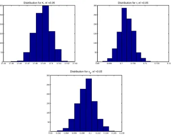
We used the constant variance data with OLS to carry out the parameter estimation calculations. The bootstrap estimates were computed with 𝑀 = 1000 and of course,
𝜃0 = (17.5,0.7,0.1). The standard errors 𝑆𝐸𝑘 and corresponding confidence intervals
[ˆ𝜃𝑘−1.96𝑆𝐸𝑘,𝜃ˆ𝑘+ 1.96𝑆𝐸𝑘] are listed in Tables 1, 2 and 3. In Figure 2 we plot the
empirical distributions for the case 𝑁𝑙 = .05 corresponding to the results in Table 2; plots in the other two cases are quite similar.
The parameter estimates and standard errors are comparable between the asymptotic theory and the bootstrapping theory for this case of constant variance. However, the computational times (given in Table 4) are two to three orders of magnitude greater for the bootstrapping method as compared to those for the asymptotic theory. For this reason, the asymptotic approach would appear (as expected from the theory) to be the more advantageous method.
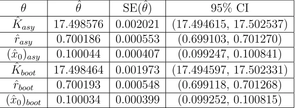
Table 1: Asymptotic and Bootstrap OLS Estimates for Constant Variance Data, w/
𝑁𝑙 = 0.01
𝜃 𝜃ˆ SE(ˆ𝜃) 95% CI
ˆ
𝐾𝑎𝑠𝑦 17.498576 0.002021 (17.494615, 17.502537)
ˆ
𝑟𝑎𝑠𝑦 0.700186 0.000553 (0.699103, 0.701270)
(ˆ𝑥0)𝑎𝑠𝑦 0.100044 0.000407 (0.099247, 0.100841)
ˆ
𝐾𝑏𝑜𝑜𝑡 17.498464 0.001973 (17.494597, 17.502331)
ˆ
𝑟𝑏𝑜𝑜𝑡 0.700193 0.000548 (0.699118, 0.701268)
Table 2: Asymptotic and Bootstrap OLS Estimates for Constant Variance Data, w/
𝑁𝑙 = 0.05
𝜃 𝜃ˆ SE(ˆ𝜃) 95% CI
ˆ
𝐾𝑎𝑠𝑦 17.486571 0.010269 (17.466444, 17.506699)
ˆ
𝑟𝑎𝑠𝑦 0.702352 0.002825 (0.696815, 0.707889)
(ˆ𝑥0)𝑎𝑠𝑦 0.098757 0.002050 (0.0947386, 0.102775)
ˆ
𝐾𝑏𝑜𝑜𝑡 17.489658 0.010247 (17.469574, 17.509742)
ˆ
𝑟𝑏𝑜𝑜𝑡 0.702098 0.002938 (0.696339, 0.707857)
(ˆ𝑥0)𝑏𝑜𝑜𝑡 0.0990520 0.002152 (0.094834, 0.103270)
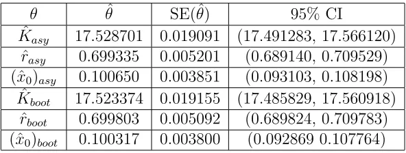
Table 3: Asymptotic and Bootstrap OLS Estimates for Constant Variance Data, w/
𝑁𝑙 = 0.1
𝜃 𝜃ˆ SE(ˆ𝜃) 95% CI
ˆ
𝐾𝑎𝑠𝑦 17.528701 0.019091 (17.491283, 17.566120)
ˆ
𝑟𝑎𝑠𝑦 0.699335 0.005201 (0.689140, 0.709529)
(ˆ𝑥0)𝑎𝑠𝑦 0.100650 0.003851 (0.093103, 0.108198)
ˆ
𝐾𝑏𝑜𝑜𝑡 17.523374 0.019155 (17.485829, 17.560918)
ˆ
𝑟𝑏𝑜𝑜𝑡 0.699803 0.005092 (0.689824, 0.709783)
(ˆ𝑥0)𝑏𝑜𝑜𝑡 0.100317 0.003800 (0.092869 0.107764)
Table 4: Computation Times (sec) for Asymptotic Theory vs. Bootstrapping
Noise Level Asymptotic Theory Bootstrapping
1% 0.017320 4.285640
5% 0.009386 4.625428
17.440 17.45 17.46 17.47 17.48 17.49 17.5 17.51 17.52 17.53 50
100 150 200 250 300
Distribution for K, nl =0.05
0.690 0.695 0.7 0.705 0.71 0.715 0.72 50
100 150 200 250 300
Distribution for r, nl =0.05
0.090 0.092 0.094 0.096 0.098 0.1 0.102 0.104 0.106 0.108 50
100 150 200 250 300
Distribution for x
0, nl =0.05
6.3
Non-constant Variance Data with GLS
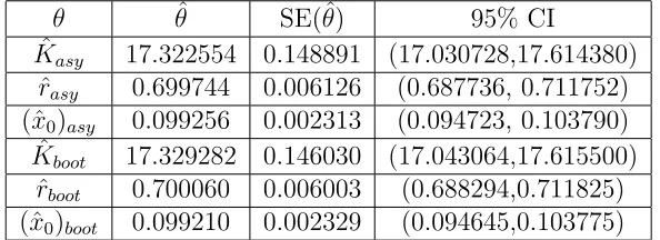
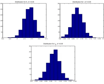
We carried out a similar set of computations for the case of non-constant variance data using a GLS formulation (in these calculations we used 1 GLS iteration). The bootstrap estimates were again computed with 𝑀 = 1000. Standard errors and corresponding confidence intervals are listed in Tables 5, 6 and 7. In Figure 3 we plot the empirical distributions for the case 𝑁𝑙 =.05 corresponding to the results in Table 6; again, plots in the other two cases are quite similar.
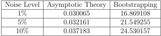
We observe that the standard errors computed from the bootstrapping method are very similar to the standard errors computed using asymptotic theory. In each of these cases the standard errors for the parameter 𝐾 are one to two orders of magnitudes greater than the standard errors for 𝑟 and 𝑥0. The computational time is also slower for the bootstrapping method, thus asymptotic theory may again be the method of choice.
Table 5: Asymptotic and Bootstrap GLS Estimates for Non-Constant Variance Data, w/ 𝑁𝑙= 0.01
𝜃 𝜃ˆ SE(ˆ𝜃) 95% CI
ˆ
𝐾𝑎𝑠𝑦 17.514706 0.028334 (17.459171, 17.570240)
ˆ
𝑟𝑎𝑠𝑦 0.70220 0.001156 (0.699934, 0.704465)
(ˆ𝑥0)𝑎𝑠𝑦 0.099145 0.000435 (0.098292,0.099999)
ˆ
𝐾𝑏𝑜𝑜𝑡 17.515773 0.027923 (17.461045, 17.570502)
ˆ
𝑟𝑏𝑜𝑜𝑡 0.702136 0.001110 (0.699960, 0.704311)
(ˆ𝑥0)𝑏𝑜𝑜𝑡 0.099160 0.000416 (0.098344, 0.099976)
Table 6: Asymptotic and Bootstrap GLS Estimates for Non-Constant Variance Data, w/ 𝑁𝑙= 0.05
𝜃 𝜃ˆ SE(ˆ𝜃) 95% CI
ˆ
𝐾𝑎𝑠𝑦 17.322554 0.148891 (17.030728,17.614380)
ˆ
𝑟𝑎𝑠𝑦 0.699744 0.006126 (0.687736, 0.711752)
(ˆ𝑥0)𝑎𝑠𝑦 0.099256 0.002313 (0.094723, 0.103790)
ˆ
𝐾𝑏𝑜𝑜𝑡 17.329282 0.146030 (17.043064,17.615500)
ˆ
𝑟𝑏𝑜𝑜𝑡 0.700060 0.006003 (0.688294,0.711825)
Table 7: Asymptotic and Bootstrap GLS Estimates for Non-Constant Variance Data, w/ 𝑁𝑙= 0.1
𝜃 𝜃ˆ SE(ˆ𝜃) 95% CI
ˆ
𝐾𝑎𝑠𝑦 17.233751 0.294422 (16.656683,17.810818)
ˆ
𝑟𝑎𝑠𝑦 0.676748 0.011875 (0.653473, 0.700024)
(ˆ𝑥0)𝑎𝑠𝑦 0.109710 0.005015 (0.099880, 0.119540)
ˆ
𝐾𝑏𝑜𝑜𝑡 17.241977 0.275328 (16.702335, 17.781619)
ˆ
𝑟𝑏𝑜𝑜𝑡 0.676694 0.011845 (0.653479, 0.699909)
(ˆ𝑥0)𝑏𝑜𝑜𝑡 0.109960 0.005031 (0.100098, 0.119821)
16.60 16.8 17 17.2 17.4 17.6 17.8 50
100 150 200 250 300
Distribution for K, nl =0.05
0.680 0.685 0.69 0.695 0.7 0.705 0.71 0.715 0.72 0.725 0.73 50
100 150 200 250 300
Distribution for r, nl =0.05
0.090 0.092 0.094 0.096 0.098 0.1 0.102 0.104 0.106 0.108 50
100 150 200 250 300
Distribution for x
0, nl =0.05
Table 8: Computation Times (sec) for Asymptotic Theory vs. Bootstrapping
Noise Level Asymptotic Theory Bootstrapping
1% 0.030065 16.869108
5% 0.032161 21.549255
10% 0.037183 24.530157
7
Using the Incorrect Assumptions on Errors
In practice, one rarely knows the form of the statistical error with any degree of certainty, so that the assumed models (3) and (9) may well be incorrect for a given data set. To obtain some information on the effect, if any, of incorrect error model assumptions on comparisons between bootstrapping and use of asymptotic theory in computing standard errors we carried out further computations.
In this section, we repeat the comparisons above for asymptotic theory and bootstrap-ping generated standard errors, but with incorrect assumptions about the error (constant or non-constant variance). Using the same data sets as created previously, we computed parameter estimates and standard errors for the constant variance data for asymptotic theory and bootstrapping using a GLS formulation, which usually is employed if non-constant variance data is suspected. Similarly, we estimated parameters and standard errors for both approaches in an OLS formulation with the non-constant variance data. In summary, we demonstrate below that if incorrect assumptions are made about the statistical model for error contained within the data, one cannot ascertain whether the correct assumption about the error has been made simply from examining the estimated standard errors. The residual plots must be examined to determine if the error model for constant or non-constant variance is reasonable. This is discussed more fully in [3] and [8, Chapter 3].
7.1
Constant Variance Data, Using GLS
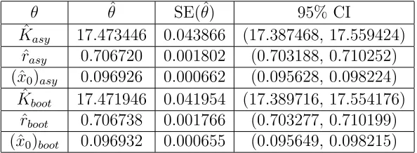
The bootstrap estimates were computed with 𝑀 = 1000 and 1 GLS iteration, with the findings reported in the tables below in a format similar to those in the previous sections. No empirical distribution plots are given here because we found they added little in the way of notable new information.
noise levels 1% to 10%, respectively. The 𝑟 and 𝑥0 standard errors also increase as the noise levels increase. These incorrectly obtained standard error estimates are larger in comparison to those obtained using an OLS formulation with the correct assumption about the error.
Table 9: Asymptotic and Bootstrap GLS Estimates for Constant Variance Data, w/
𝑁𝑙 = 0.01
𝜃 𝜃ˆ SE(ˆ𝜃) 95% CI
ˆ
𝐾𝑎𝑠𝑦 17.473446 0.043866 (17.387468, 17.559424)
ˆ
𝑟𝑎𝑠𝑦 0.706720 0.001802 (0.703188, 0.710252)
(ˆ𝑥0)𝑎𝑠𝑦 0.096926 0.000662 (0.095628, 0.098224)
ˆ
𝐾𝑏𝑜𝑜𝑡 17.471946 0.041954 (17.389716, 17.554176)
ˆ
𝑟𝑏𝑜𝑜𝑡 0.706738 0.001766 (0.703277, 0.710199)
(ˆ𝑥0)𝑏𝑜𝑜𝑡 0.096932 0.000655 (0.095649, 0.098215)
Table 10: Asymptotic and Bootstrap GLS Estimates for Constant Variance Data, w/
𝑁𝑙 = 0.05
𝜃 𝜃ˆ SE(ˆ𝜃) 95% CI
ˆ
𝐾𝑎𝑠𝑦 17.486405 0.169916 (17.153369, 17.819441)
ˆ
𝑟𝑎𝑠𝑦 0.696663 0.006939 (0.683063, 0.710263)
(ˆ𝑥0)𝑎𝑠𝑦 0.103291 0.002722 (0.097956, 0.108625)
ˆ
𝐾𝑏𝑜𝑜𝑡 17.477246 0.165693 (17.152487, 17.802004)
ˆ
𝑟𝑏𝑜𝑜𝑡 0.696828 0.006770 (0.683558, 0.710098)
Table 11: Asymptotic and Bootstrap GLS Estimates for Constant Variance Data, w/
𝑁𝑙 = 0.1
𝜃 𝜃ˆ SE(ˆ𝜃) 95% CI
ˆ
𝐾𝑎𝑠𝑦 17.648739 0.504870 (16.659193, 18.638285)
ˆ
𝑟𝑎𝑠𝑦 0.680706 0.019755 (0.641985, 0.719427)
(ˆ𝑥0)𝑎𝑠𝑦 0.106576 0.008143 (0.090616, 0.122537)
ˆ
𝐾𝑏𝑜𝑜𝑡 17.668510 0.490496 (16.707137, 18.629882)
ˆ
𝑟𝑏𝑜𝑜𝑡 0.681164 0.018922 (0.644077, 0.718251)
(ˆ𝑥0)𝑏𝑜𝑜𝑡 0.106784 0.007835 (0.091427, 0.122140)
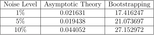
Table 12: Computation Times (sec) for Asymptotic Theory vs. Bootstrapping
Noise Level Asymptotic Theory Bootstrapping
1% 0.021631 17.416247
5% 0.019438 21.073697
7.2
Non-constant Variance Data, Using OLS
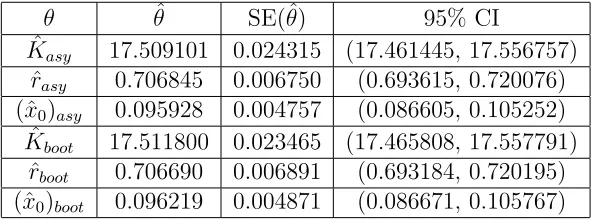
The bootstrap estimates were again computed with𝑀 = 1000. When the error estimates for data sets with non-constant variance are estimated using OLS, the estimates are comparable for the asymptotic theory and bootstrapping methods. In comparing these estimates to the error estimates obtained under accurate assumptions, we observe that under the incorrect error model assumption, the standard error for 𝐾 is always smaller (though comparable) regardless of the noise level, while the corresponding 𝑟 and 𝑥0 standard errors are always larger. For 𝑥0, the standard error under OLS is an order of magnitude larger as compared to the GLS case (non-constant variance).
Table 13: Asymptotic and Bootstrap OLS Estimates for Non-Constant Variance Data, w/ 𝑁𝑙= 0.01
𝜃 𝜃ˆ SE(ˆ𝜃) 95% CI
ˆ
𝐾𝑎𝑠𝑦 17.509101 0.024315 (17.461445, 17.556757)
ˆ
𝑟𝑎𝑠𝑦 0.706845 0.006750 (0.693615, 0.720076)
(ˆ𝑥0)𝑎𝑠𝑦 0.095928 0.004757 (0.086605, 0.105252)
ˆ
𝐾𝑏𝑜𝑜𝑡 17.511800 0.023465 (17.465808, 17.557791)
ˆ
𝑟𝑏𝑜𝑜𝑡 0.706690 0.006891 (0.693184, 0.720195)
(ˆ𝑥0)𝑏𝑜𝑜𝑡 0.096219 0.004871 (0.086671, 0.105767)
Table 14: Asymptotic and Bootstrap OLS Estimates for Non-Constant Variance Data, w/ 𝑁𝑙= 0.05
𝜃 𝜃ˆ SE(ˆ𝜃) 95% CI
ˆ
𝐾𝑎𝑠𝑦 17.301393 0.122316 (17.061653, 17.541133)
ˆ
𝑟𝑎𝑠𝑦 0.694052 0.033396 (0.628596, 0.759508)
(ˆ𝑥0)𝑎𝑠𝑦 0.105893 0.025879 (0.055171, 0.156615)
ˆ
𝐾𝑏𝑜𝑜𝑡 17.291459 0.118615 (17.058973, 17.523945)
ˆ
𝑟𝑏𝑜𝑜𝑡 0.697367 0.034670 (0.629413, 0.765320)
Table 15: Asymptotic and Bootstrap OLS Estimates for Non-Constant Variance Data, w/ 𝑁𝑙= 0.1
𝜃 𝜃ˆ SE(ˆ𝜃) 95% CI
ˆ
𝐾𝑎𝑠𝑦 17.081926 0.262907 (16.566629, 17.597223)
ˆ
𝑟𝑎𝑠𝑦 0.727602 0.078513 (0.573717, 0.881487)
(ˆ𝑥0)𝑎𝑠𝑦 0.082935 0.047591 (-0.010343, 0.176213)
ˆ
𝐾𝑏𝑜𝑜𝑡 17.095648 0.250940 (16.603807, 17.587490)
ˆ
𝑟𝑏𝑜𝑜𝑡 0.733657 0.081852 (0.573228, 0.894087)
(ˆ𝑥0)𝑏𝑜𝑜𝑡 0.094020 0.054849 (-0.013484, 0.201524)
Table 16: Computation Times (sec) for Asymptotic Theory vs. Bootstrapping
Noise Level Asymptotic Theory Bootstrapping
1% 0.008697 5.075417
5% 0.009440 6.002897
8
The Corrective Nature of Bootstrapping
Covari-ance Estimates
When estimating 𝜃 using GLS, there may be more error in the estimated covariance matrix, ˆΣ𝑛(ˆ𝜃), due to the estimation of weights. Recalling Theorem 4 from Carroll, Wu,
and Ruppert [13, p. 1048], originally given in [24, p. 815], we can write the bootstrap estimate of the covariance matrix as
𝐶𝑜𝑣(ˆ𝜃𝑏𝑜𝑜𝑡) = ˆΣ𝑛(ˆ𝜃) +𝑛−1𝜎02Λ(𝐹) +𝑂𝑝(𝑛−3/2),
where Λ(𝐹) is an unknown positive-definite matrix. As a result the bootstrapping covariance matrix is generally thought to be more accurate than the asymptotic theory estimate due to the corrective term 𝑛−1𝜎2
0Λ(𝐹). The corrective term is discussed for the linear model in [13, p. 1050], and for the nonlinear model in [12, p. 28] where the standardized residuals are defined by
𝜖𝑖 =
(𝑦𝑖−𝑓(𝑥𝑖, 𝜃))
𝜎𝑔(𝑓(𝑥𝑖, 𝜃), 𝑥𝑖, 𝜃)
.
In simulations reported in previous sections, we found that our results did not necessarily meet expectations consistent with the theory presented by Carroll, Wu, and Ruppert [13]. After further examination of the theory, we find that the theory is presented and discussed in detail for a linear model. To further explore this, we linearized our original model (𝑓(𝑡, 𝜃)) about𝜃 =𝜃∗, and re-ran our simulations. As a result of the linearization
we have the following new model
𝑦=𝐹0(𝑡, 𝜃∗) +𝐹1(𝑡, 𝜃∗)(𝐾 −𝐾∗) +𝐹2(𝑡, 𝜃∗)(𝑟−𝑟∗) +𝐹3(𝑡, 𝜃∗)(𝑥0 −𝑥∗0), (12) where 𝐹0 = 𝑓(𝑡, 𝜃), 𝐹1 = ∂𝑓∂𝑘(𝑡,𝜃), 𝐹2 = ∂𝑓∂𝑟(𝑡,𝜃), and 𝐹3 = ∂𝑓∂𝑥(𝑡,𝜃0). Note that 𝜃0 =
{𝐾∗, 𝑟∗, 𝑥∗
0} = {17.5,0.7,0.1}. We considered this new model and performed the same computational analysis as described earlier. At each simulation while the values for the bootstrapping standard errors are similar, their specific values would vary in comparison to the asymptotic theory standard errors, which are the same for repeated simulations. For example, during the first run all bootstrapping computed standard errors for 𝐾, 𝑟, 𝑥0 would be larger in comparison to the asymptotic theory estimates, while on the next run only 𝐾, 𝑟 would have corresponding larger estimates. We performed a Monte Carlo analysis, for 1000 trials using M=250, to find the average behavior of the bootstrapping standard errors. We performed these Monte Carlo simulations on the same time inter-val 𝑇 ∈ [0,20], at 10% noise, where 𝑛 = 20,25,30,35 and 40. When comparing this average bootstrapping standard error with the asymptotic standard error for 𝐾, 𝑟, 𝑥0 at 𝑛 = 20,25,30,35 and 40, we observe that the bootstrapping estimates are larger (as expected) for parameters 𝐾, 𝑟, but slightly smaller (not expected) for the parameter 𝑥0. We would expect that the theory presented in [13] would be observed at lower values of
𝑛 due to the correction term𝑛−1𝜎2
0Λ(𝐹); however, the inverse problem is very unstable at this sample size because it appeared that at least 9 data points are needed for each parameter that is being estimated in this problem. (We remark that in general the correlation between the number of data points required per parameter estimated is not easy to compute and is very much problem dependent–this is only one of a number of difficulties arising in such problems–see [9, p. 87] for discussions. Indeed this problem is one of active research interest in the areas of sensitivity functions [4, 5, 6, 28] and design of experiments.) We expected to observe theory-consistent SE at the higher values of 𝑛, because we have three parameters estimates. Although we observe the desired theoret-ical behavior for 2 out of 3 of the parameters, the lack of data for the inverse problem could be the reason we do not observe this corrective theory for all parameters.
To better understand the fluctuations in bootstrapping standard errors among the three parameters, we ran the Monte Carlo simulations for the estimation of just one param-eter. When only the parameter 𝑟 was estimated, the bootstrapping standard errors were larger than those of asymptotic theory for every case, using 𝑛 = 10,15,20 and 25 time points. These simulations supported the theory of the corrective nature of boot-strapping. We also examined the standard errors when only estimating 𝑥0, again for
of magnitude for the bootstrapping method, as compared to asymptotic theory. This example provides some evidence that the corrective nature of the bootstrap may only be realized in certain situations.
Carroll and Ruppert [12, p. 15–16] describe the following result for the behavior of GLS with a particular non-constant variance model. If the data points have higher variance in a neighborhood of importance for estimating a specific parameter (for our example the region of rapidly increasing slope is important for estimating 𝑟), then the weights in GLS heavily influence the estimate and the standard error. Based on our computational findings, we are inclined to think that this local variance also influences whether or not the bootstrapping estimate will be “corrective”. If the GLS weights are not as important, then the bootstrap error estimate will not exhibit the corrective term of the covariance properly.
We ran some simulations for both the linearized and nonlinear models to test this hy-pothesis. For our example, in the solution to the logistic equation there are three regions each of importance for estimating one of the parameters. Region I is important for esti-mation of 𝑥0 and is the region where𝑥(𝑡) is near 𝑥0, located near the initial time points before the slope begins to increase significantly. Region II data influences heavily the estimation of 𝑟 and is located in the area of the increasing slope. Region III is located where the solution approaches the steady state𝑥(∞) = 𝐾. Due to the manner in which our simulated non-constant variance data was modeled, Region I had little variation in comparison to Regions II and III. This low variation in Region I led us to believe that increasing the variance in this region would demonstrate the corrective nature of the bootstrapping estimate. We subsequently created data sets (linear and nonlinear) where variance was only increased in Region I and remained the same in Regions II and III. For these new data sets all of the bootstrapping standard errors were larger than the asymptotic standard errors and hence exhibited the theoretically predicted corrective nature of bootstrapping generated standard errors. We also created data sets where there was less variance around the asymptote 𝑥 = 𝐾 (region III), and for those data sets the bootstrapping generated standard error was smaller when compared to the asymptotic theory standard error. This leads us to believe that local variance strongly influences the presence or not of the corrective nature of the bootstrapping estimate.
9
Summary of Literature on the Asymptotic Nature
of the Bootstrapping Estimate
directly from the sample (ex: mean, and variance). In this situation, there is no model for the data therefore no inverse problem is needed to estimate the parameters. The results that follow are of interest for the general bootstrapping method, but are not directly applicable for parameter estimation for a nonlinear model using bootstrapping. Bickel and Freedman [11] give insight to asymptotic theory for the general bootstrapping method in a population 𝑌1, ..., 𝑌𝑛, where 𝑌𝑖 =𝑡𝑖+𝜖𝑖 and iid with empirical distribution
𝐹𝑛. It is assumed that 𝐹𝑛 has finite mean,𝜇𝑛, and finite positive variance𝜎𝑛2 where the
standard deviation is
𝑠2 𝑛= 1 𝑛 𝑛 ∑ 𝑖=1
(𝑌𝑖−𝜇𝑛)2.
Then a conditionally independent bootstrapping sample of size𝑛𝑏 sampled from the
pop-ulation{𝑌1, ..., 𝑌𝑛}is defined as{𝑌1∗, ..., 𝑌𝑛∗𝑏}, where𝑠 ∗
𝑛𝑏 =
1
𝑛𝑏
∑𝑛𝑏
𝑖=1(𝑌𝑖∗−𝜇∗𝑛𝑏)
2, and𝜇∗
𝑛𝑏 =
1
𝑛𝑏
∑𝑛𝑏
𝑖=1𝑌𝑖∗ is an estimate for 𝜇𝑛. From here a pivotal quantity 𝑄𝑛 = √
𝑛(𝜇𝑛 −𝜇)/𝑠𝑛
can be estimated from 𝑄∗
𝑛𝑏 =
√
𝑛𝑏(𝜇∗𝑛𝑏 −𝜇𝑛)/𝑠 ∗
𝑛𝑏. Note that 𝑛 is the number of data
points in the population while 𝑛𝑏 is the bootstrapping sample size which does not have
to equal 𝑛, and𝑄𝑛 converges weakly to𝒩(0,1), given 𝜇is known, by the Central Limit
Theorem. Bickel and Freedman report the asymptotic properties of 𝑄∗
𝑛𝑏 and find its
asymptotic convergence to be in accordance with the convergence of 𝑄𝑛. The following
theorems are as a result of the previously discussed findings.
Theorem 2.1 [11, p. 1197] Suppose 𝑌1, 𝑌2, ... are iid and have finite positive variance
𝜎2. Along almost all sample sequences 𝑌
1, 𝑌2, ..., given (𝑌1, .., 𝑌𝑛), as 𝑛 and 𝑛𝑏 tend to ∞ we have:
(a)The conditional distribution of √𝑛𝑏(𝜇∗𝑛𝑏 −𝜇𝑛) converges weakly to 𝒩(0, 𝜎
2) and
(b) 𝑠∗
𝑛𝑏 converges to 𝜎 in conditional probability.
Theorem 2.2 [11, p. 1197] Let 𝑌1, 𝑌2, ..., be independent with a common distribution in 𝑅𝑑. Suppose 𝐸{∣∣𝑌
1∣∣2} < ∞. Let 𝐹𝑛 be the empirical distribution of 𝑌1, ..., 𝑌𝑛, and
let 𝑌∗
1, .., 𝑌𝑛∗𝑏 be conditionally independent, with common distribution 𝐹𝑛. Then along
almost all sample sequences, as 𝑛𝑏 and 𝑛 tend to infinity:
(a) The conditional distribution of √𝑛𝑏
( 1
𝑛𝑏
∑𝑛𝑏
𝑖=1𝑌𝑖∗− 1𝑛
∑𝑛
𝑗=1𝑌𝑗 )
converges weakly to the d-dimensional normal distribution with mean 0, and variance-covariance matrix equal to the theoretical variance variance-covariance matrix 𝑌1
(b) The empirical variance-covariance matrix of 𝑌∗
1, .., 𝑌𝑛∗𝑏 converges in conditional
prob-ability to the theoretical variance-covariance matrix of 𝑌1.
of explanatory variables associated with the data (for example 𝑡(𝑖) = (1, 𝑡
𝑖, 𝑡2𝑖, . . . 𝑡𝑝𝑖−1)′),
and 𝜃 is a𝑝-vector of unknown parameters. Let𝑇′ = (𝑡(1), . . . , 𝑡(𝑛)),ℎ
𝑖 =𝑡(𝑖)
′
(𝑇′𝑇)−1𝑡(𝑖), and ℎ𝑚𝑎𝑥 = 𝑚𝑎𝑥𝑖≤𝑛ℎ𝑖. Let 𝑣boot be the variance estimator of ˆ𝜃𝑏𝑜𝑜𝑡, the bootstrapping
estimate of 𝜃. The OLS estimate of 𝜃 is denoted by ˆ𝜃𝑂𝐿𝑆.
In addition, we define the Mallows’ distance (as shown on pg 73 [26]) on ℱ𝑟,𝑠 = {𝐺 ∈ ℱℝ𝑠::
∫
∥𝑡∥𝑟𝑑𝐺(𝑡)<∞}. The two distributions𝐻 and𝐺inℱ
𝑟,𝑠 have Mallows’ distance,
˜
𝜌𝑟(𝐻, 𝐺) = inf
𝒯𝑋,𝑌
(𝐸∥𝑋−𝑌∥𝑟)1/𝑟,
where 𝒯𝑋,𝑌 is the collection of all possible joint distributions of (𝑋, 𝑌), if𝑋 and𝑌 have
marginal distributions 𝐻 and 𝐺, respectively.
Shao and Tu give us the following two theorems that prove the bootstrapping estimator of variance of the parameter is consistent, as is the bootstrapping distribution estimator [26].
Theorem 7.3.i [26, p. 317]: Consistency of 𝑣boot. If 𝑇′𝑇 → ∞, ℎ
𝑚𝑎𝑥 → 0, and we have constant variance (𝜎2𝑖 = 𝜎2 for all 𝑖), then
𝑣boot/var(𝑐′𝜃ˆ𝑂𝐿𝑆) →𝑝 1, where 𝑐 is a vector of arbitrary constants. Additionally, we
have that bias(𝑣boot)/var(𝑐′𝜃ˆ𝑂𝐿𝑆) = 𝑂(𝑛−1) and var(𝑣boot)/[var(𝑐′𝜃ˆ𝑂𝐿𝑆)]2 = 𝑂(𝑛−1), if
𝐸(𝜖4
𝑖 <∞).
Theorem 7.6[26, p. 320]: Consistency of the distribution estimator based on bootstrap-ping the residuals.
Assume 𝑇′𝑇 → ∞, ℎ
𝑚𝑎𝑥 →0, and the 𝜖𝑖 are i.i.d.. Then
˜
𝜌2(𝐻𝑏𝑜𝑜𝑡, 𝐻𝑛)→𝑎.𝑠. 0,
where𝐻𝑛is the distribution of (𝑇′𝑇)1/2(ˆ𝜃𝑂𝐿𝑆−𝜃) and𝐻𝑏𝑜𝑜𝑡 is the bootstrap distribution
of (𝑇′𝑇)1/2(ˆ𝜃
𝑏𝑜𝑜𝑡−𝜃ˆ𝑂𝐿𝑆).
Shao and Tu state that these consistency results can be generalized for nonlinear models in [26, p. 331, 335–337], though no rigorous proof is given.
9.1
Iterative Bootstrap Asymptotics
Earlier we discussed asymptotics for bootstrapping methods in reference to sample size,
𝑛, now we will highlight some discussion on the asymptotics in reference to 𝑀 the number of bootstrapping samples. Efron and Tibrishani state the bootstrap method is asymptotically efficient in [17, p. 395] , meaning that as 𝑀 −→ ∞, ˆ𝑆𝐸(𝑀)(ˆ𝜃𝑏𝑜𝑜𝑡) −→
ˆ
𝑆𝐸∞(ˆ𝜃𝑏𝑜𝑜𝑡), the ideal bootstrap estimate of standard error in [17, p. 50]. In addition,
parameter estimates [17, p. 395]. For a general bootstrap method, 𝑀 = 50 is sufficient to estimate 𝜃, 𝑀 = 200 is sufficient to estimate the standard error, and 𝑀 = 1000 is sufficient to estimate confidence intervals for 𝜃 as reported in [17, p. 52, 164].
9.2
Determining Iterative Size for the Bootstrapping Estimate
Let 𝐻𝑏𝑜𝑜𝑡(𝑥) represent the distribution of ˆ𝜃𝑏𝑜𝑜𝑡 conditional to the empirical distribution𝐹. Let 𝐻𝑀
𝑏𝑜𝑜𝑡(𝑥) be the approximation of 𝐻𝑏𝑜𝑜𝑡(𝑥) at the 𝑀𝑡ℎ iterate. The following
result holds
sup
𝑥 ∣𝐻𝑀
𝑏𝑜𝑜𝑡(𝑥)−𝐻𝑏𝑜𝑜𝑡(𝑥)∣=𝜖𝑛+
√
𝑀−1𝑙𝑜𝑔 𝑙𝑜𝑔𝑀
and
sup 0<𝑡<1∣(𝐻
𝑀
𝑏𝑜𝑜𝑡)−1(𝑡)−(𝐻𝑏𝑜𝑜𝑡)−1(𝑡)∣=𝑂(𝜖𝑛+
√
𝑀−1𝑙𝑜𝑔 𝑙𝑜𝑔𝑀),
where 𝜖𝑛= sup𝑥∣𝐻𝑏𝑜𝑜𝑡𝑀 (𝑥)−𝐻𝑏𝑜𝑜𝑡(𝑥)∣, established by Shi, Wu and Chen [27] as shown in
Shao and Tu [26, p. 210]. In addition 𝑀 is determined using the following relationship:
𝑀−1𝑙𝑜𝑔 𝑙𝑜𝑔𝑀 =𝑜(𝜖2
𝑛).
10
Summary
Based on our computational experience with a known example we make the follow-ing summary remarks/conclusions. Asymptotic theory and bootstrappfollow-ing are distinct methods for quantifying uncertainty in parameter estimates. Asymptotic theory is al-ways faster computationally than bootstrapping; however, this is the only definitive comparison that can be made. Depending on the type of data set, one method may be more favorable than the other. For constant variance data using OLS there is no clear advantage in using bootstrapping over asymptotic theory. However, for a complex system it may be too complicated to compute the sensitivities needed for asymptotic theory; then bootstrapping may be more reasonable for estimating the standard er-ror. If computation time is already a concern, but sensitivities can be computed, then asymptotic theory may be advantageous.
Given that the statistical model correctly assumes non-constant variance, the parameters are estimated using GLS, and the asymptotic theory error estimates and the bootstrap-ping error estimates are comparable. If local variation in the data points is large in a region of importance for estimation of a parameter, then the bootstrapping covariance estimate may contain a corrective term of significance. In that situation, the standard errors for bootstrapping will be larger than those of asymptotic theory, and hence more
conservative and also more accurate. If the local variation in the data is low in a region
theory depends onlocal variation in the data in regions of importance for the estimation of the parameters.
Acknowledgments
This research was supported by the National Institutes of Health in part under grant number R01AI071915-07 from the National Institute of Allergy and Infectious Diseases and in part by the Air Force Office of Scientific Research under grant number FA9550-09-1-0226. The research of D.R. was also supported in part by a Graduate Fellowship under the Initiative for Maximizing Student Diversity (IMSD) program grant PAR-06-553 funded by the NIH.
References
[1] G.Anger, Inverse Problems in Differential Equations, Plenum Press, New York, 1990.
[2] H. T. Banks, M. W. Buksas and T. Lin, Electromagnetic Material Interrogation
Using Conductive Interfaces and Acoustic Wavefronts, SIAM FR21, Philadelphia,
2002.
[3] H. T. Banks, M. Davidian, J. R. Samuels Jr., and K. L. Sutton, An inverse problem statistical methodology summary, CRSC Technical Report, CRSC-TR08-01, NCSU, January, 2008; Chapter 11 in Statistical Estimation Approaches in Epidemiology, (edited by Gerardo Chowell, Mac Hyman, Nick Hengartner, Luis M.A Bettencourt and Carlos Castillo-Chavez), Springer, Berlin Heidelberg New York, 2009, 249–302.
[4] H. T. Banks, S. Dediu and S. E. Ernstberger, Sensitivity functions and their uses in inverse problems, CRSC Tech Report, CRSC-TR07-12, NCSU, July, 2007; J.
Inverse and Ill-posed Problems, 15 (2007), 683–708.
[5] H. T. Banks, S. Dediu, S. L. Ernstberger, F. Kappel, A new approach to optimal design problems, CRSC Technical Report CRSC-TR08-12, NCSU, September, 2008.
[6] H. T. Banks, S. L. Ernstberger and S. L. Grove, Standard errors and confidence intervals in inverse problems: sensitivity and associated pitfalls, J. Inverse and
Ill-posed Problems,15 (2007), 1–18.
[7] H. T. Banks and K. Kunsich, Estimation Techniques for Distributed Parameter
Systems, Boston:Birkha¨user, 1989.
[8] H. T. Banks and H. T. Tran, Mathematical and Experimental Modeling of Physical
[9] D. M. Bates, Nonlinear Regression Analysis and its Applications, J. Wiley & Sons, Somerset, NJ, 1988.
[10] J. Baumeister, Stable Solutions of Inverse Problems, Vieweg, Braunschweig, 1987.
[11] P. Bickel and D. Freedman, Some asymptotic theory for the bootstrap, The Annals
of Statistics,9(6) (1981), 1196–1217.
[12] R. J. Carroll and D. Ruppert, Transformation and Weighting in Regression, Chap-man & Hall, London, 1988.
[13] R. J. Carroll, C. F. J. Wu and D. Ruppert, The effect of estimating weights in Weighted Least Squares,J. Amer. Statistical Assoc., 83 (1988), 1045–1054.
[14] G. Casella and R. L. Berger, Statistical Inference, Duxbury, California, 2002.
[15] M. Davidian, Nonlinear Models for Univariate and Multivariate Response, ST 762 Lecture Notes, Chapters 9 and 11, 2007; http://www4.stat.ncsu.edu/ david-ian/courses.html
[16] M. Davidian and D. M. Giltinan,Nonlinear Models for Repeated Measurement Data,
Chapman & Hall, London, 1995.
[17] B. Efron and R. J. Tibshirani, An Introduction to the Bootstrap, Chapman & Hall/CRC Press, Boca Raton, 1998.
[18] H. W. Engl and C. W. Groetsch (eds.), Inverse and Ill-posed Problems, Academic Press, Orlando, 1987.
[19] C. W. Groetsch, Inverse Problems in the Mathematical Sciences, Vieweg, Braun-schweig, 1993.
[20] C. W. Groetsch, The Theory of Tikhonov Regularization for Fredholm Equations of
the First Kind, Pitman, London, 1984.
[21] B. Hoffman, Regularization for Applied Inverse and Ill-posed Problems, Teubner, Leipzig, 1986.
[22] M. Kot, Elements of Mathematical Ecology, Cambridge University Press, Cam-bridge, 2001.
[23] N. Matloff, R. Rose, R. Tai, A comparison of two methods for estimating optimal weights in regression analysis, J. Statist. Comput. Simul.,19 (1984), 265–274.
[24] T. J. Rothenberg, Approximate normality of generalized least squares estimates,
[25] G. A. F. Seber and C. J. Wild, Nonlinear Regression, Wiley-Interscience, Hoboken, NJ, 2003.
[26] J. Shao and D. Tu,The Jackknife and Bootstrap, Springer-Verlag, New York, 1995.
[27] X. Shi, J. Chen, and C. F. J. Wu, Weak and strong representations for quantile processes from finite populations with applications to simulation size in resampling methods,Canadian J. Statist., 18 (1990), 141–148.
[28] K. Thomaseth and C. Cobelli, Generalized sensitivity functions in physiological system identification, Annals of Biomedical Engineering, 27 (1999), 607–616.
[29] A. N. Tikhonov and V. Y. Arsenin, Solutions of Ill-posed Problems, Winston and Sons, Washington, 1977.