Copyright1998 by the Genetics Society of America
Genealogical Inference From Microsatellite Data
Ian J. Wilson*
,†and David J. Balding
†*School of Biological Sciences, Queen Mary and Westfield College, University of London, London E1 4NS, England and
†Department of Applied Statistics, University of Reading, Reading RG6 6FN, England
Manuscript received November 21, 1997 Accepted for publication June 3, 1998
ABSTRACT
Ease and accuracy of typing, together with high levels of polymorphism and widespread distribution in the genome, make microsatellite (or short tandem repeat) loci an attractive potential source of information about both population histories and evolutionary processes. However, microsatellite data are difficult to interpret, in particular because of the frequency of back-mutations. Stochastic models for the underlying genetic processes can be specified, but in the past they have been too complicated for direct analysis. Recent developments in stochastic simulation methodology now allow direct inference about both historical events, such as genealogical coalescence times, and evolutionary parameters, such as mutation rates. A feature of the Markov chain Monte Carlo (MCMC) algorithm that we propose here is that the likelihood computations are simplified by treating the (unknown) ancestral allelic states as auxiliary parameters. We illustrate the algorithm by analyzing microsatellite samples simulated under the model. Our results suggest that a single microsatellite usually does not provide enough information for useful inferences, but that several completely linked microsatellites can be informative about some aspects of genealogical history and evolutionary processes. We also reanalyze data from a previously published human Y chromosome microsatellite study, finding evidence for an effective population size for human Y chromosomes in the low thousands and a recent time since their most recent common ancestor: the 95% interval runs from z15,000 to 130,000 years, with most likely values around 30,000 years.
P
ATTERNS of heritable genetic variation in contem- relationships, but does not provide a basis for assessing porary samples can provide information both about the uncertainty associated with inferences.parameters of evolutionary processes and about details Recently, inferential methods that use the coalescent of the genealogical history of the sample. Data from the (Kingman1982;Hudson1991) to model explicitly the
male-specific part of the human Y chromosome, for genealogical relationships underlying a genetic sample example, can provide evidence both about mutation have become available (Griffiths and Tavare´ 1994;
rates and about the number and reproductive behavior Kuhneret al. 1995).Tavare´ et al. (1997) present
com-of human males. When combined with information putational methods for genealogical inference under from mitochondrial, autosomal, and X chromosome the assumptions of the coalescent model with infinite-loci, additional insights about recent human evolution- sites mutation, so that back-mutation is assumed to not ary history may be obtained. occur. Microsatellite loci present a particular challenge Extracting historical and evolutionary information to genealogical inference because these loci form an from the genetic data is, however, difficult, due to the important source of highly polymorphic molecular ge-complex interaction of the underlying genetic pro- netic data (JarneandLagoda1996), but the mutation
cesses. Traditionally, the interpretation of genetic sam- process is such that back-mutations cannot reasonably ples has been based on summary statistics, such as heter- be ignored.Nielsen(1997) developedGriffithsand
ozygosity or pairwise measures of identity (Nei 1987; Tavare´
’s (1994) algorithm to obtain maximum
likeli-Slatkin 1995). Such an approach can waste much of
hood estimates of the scaled mutation parameteru at the information contained in the data (Felsenstein
microsatellite loci. The method was found to be compu-1992). Intuitively, this is because pairwise measures of tationally costly, even for a single locus, making accurate identity do not explicitly take account of the ancestral estimation difficult.
relationships underlying the data (Donnelly 1996).
Here, we present a computationally tractable method For microsatellite data, a network can be constructed for drawing inferences from microsatellite data, not only (Cooper et al. 1996; Zerjal et al. 1997) that displays
aboutubut also about population histories. Very briefly, some of the structure of the data and suggests historical the method is based on the coalescent model of geneal-ogy together with a ladder (or stepwise) model of micro-satellite mutation and is implemented via a Markov Corresponding author: David J. Balding, Department of Applied
Statis-chain Monte Carlo (MCMC) simulation algorithm.
tics, University of Reading, PO Box 240, Reading RG6 6FN, England.
E-mail: [email protected] In the following section we start by outlining the
lescent-with-ladder-mutation modeling framework and coalescent, assumes neutrality, random mating, and a constant, large population size. These assumptions can the process of drawing inferences from microsatellite
data under this model. FollowingTavare´ et al. (1997), each be weakened to some extent and at some
computa-tional cost. However, the novelty of this article is the we adopt a fully probabilistic approach in which the
uncertainty about an unknown parameter is expressed introduction of a model for microsatellite mutation, and to simplify the presentation of this development we in terms of its probability distribution, given the data
and the model. As well as making efficient use of all work primarily with the standard coalescent.
Time in the coalescent model is measured in units the available information, another important advantage
of this approach is interpretability. For scalar parameters, of N generations, where N is the (fixed and large) popu-lation size. Tracing backward in time the lineages of either singly or in combination, inferences are naturally
presented visually, in terms of probability density curves each gene in a sample of size n, the time t1until the first “coalescence” of two lineages at a common ancestor or surfaces. Even very complex unknowns, for example,
the entire genealogy of the sample, can be described has the exponential distribution with mean 2/n(n 2 1). Continuing backward in time, the time t2 between either in terms of probability density curves for
impor-tant features, such as height or total branch length, or the first and the second coalescences has the exponen-tial distribution with mean 2/(n2 1)(n 2 2), and so in terms of pictures of a sample of realizations from the
probability distribution. A further advantage of a fully forth, until the time tn21between the final two coales-cences (i.e., the time during which the sample has ex-probabilistic analysis is flexibility. For example,
infer-ences about the genealogical tree or about the effective actly two ancestors) has the exponential distribution with mean 1. Crucially, each of these times is indepen-population size, or both, can be obtained, according to
the goals of the investigator. dent of the other times. Hence the joint probability density of the coalescence times t1, . . . , tn21is In the recent past, fully probabilistic analyses of
com-plex genetic processes were not computationally
feasi-ble. While computational cost remains an issue, ad- p(t1, . . . , tn21)5
p
n21i51
1
n 112i
2
2
exp1
21
n1 12 i 2
2
ti2
. vances in stochastic simulation methodology, such as(1) MCMC algorithms, now allow problems of substantial
size and complexity to be tackled. One important fea- Because all pairs of lineages remaining at any time are ture of the MCMC algorithm that we propose here is equally likely to coalesce, p(t1, . . . , tn21) is proportional that the allelic type of the ancestral gene at each coales- to the probability density, under the coalescent model, cence is assigned and successively updated according to of any (labeled) genealogy with the coalescence times its conditional probabilities. This simplifies the likeli- t1, . . . , tn21.
hood computations, which in turn allow flexibility in Equation 1 pertains to the predata coalescent, in the choice of algorithms for stepping through the space which the sample size n is fixed but the allelic types are of candidate trees. not yet observed. Once the allelic types are known, the The quality of genealogical inference that can be coalescent probabilities are altered: evaluating the up-achieved under ideal circumstances is investigated using dated probabilities after observing a sample of microsat-data simulated from the model. The method is then ellite data is the primary goal of this article. A particular illustrated by reanalyzing the data of Cooper et al. feature of the predata coalescent is that most of the
(1996) for five microsatellite loci on the human Y chro- lineages coalesce relatively quickly. (In other words, mosome. Because of the complexities of the genetic most branches are short.) On the other hand, the time phenomena under study, we find that data from a single period during which the tree has just two lineages is on microsatellite locus do not suffice for accurate infer- average 1 coalescent unit, more than half the mean ences, even when the modeling assumptions hold ex- height of the coalescent tree. Another notable feature actly. However, if data from a number of completely of the predata coalescent is the high variability in tree linked loci are available and the mutation process can height: its standard deviation is about 60% of the mean be assumed to be the same at each locus, then much height for typical values of n. SeeDonnellyandTavare´
more precise inferences can be made. (1995) and references therein for further details of the coalescent model.
Microsatellite mutations:Given the genealogy, muta-THE MODEL
tions in the standard coalescent are assumed to occur Genealogies and the coalescent:Interpreting genetic independently and at constant rateu/2, where data requires an understanding of the patterns of shared u 5
2Nm ancestry among the genes in the sample. Currently, the
most successful mathematical description of the genea- andmdenotes the mutation rate per gene per genera-logical processes underlying these patterns is provided tion. This means that the number of mutations in any by the so-called coalescent model. section of the tree with total branch length t has the
Although additional variation can be distinguished to model the background information before D is ob-served, then updating this prior distribution, via Bayes’ in some cases, microsatellite alleles are usually
charac-terized by the copy number of the repeat motif. For the rule, to incorporate the information conveyed by D. The coalescent model specifies a probability distribu-data ofCooperet al. (1996) discussed below, the repeat
motif is the four-base sequence GATA. tion forY. This distribution can be thought of as a prior distribution for the genealogical tree, which should be Mutations of microsatellite alleles are thought to be
due predominantly to polymerase slippage (Levinson updated in the light of the data D. Information aboutm
obtained from pedigree studies, such as those described andGutman1987;Dover1996), which produces
mu-tant alleles close in length to the original; the mumu-tant above, can be summarized by a probability density curve that would usually be smooth and unimodal. Informa-alleles differ by whole copies of the repeat motif. Direct
studies of mutations using a large number of parent- tion about N is more difficult to specify, because N should be interpreted as an effective, rather than actual, offspring triplets (WeberandWong1993) for
autoso-mal microsatellites, and using pedigrees over larger population size. However, previous genetic studies, to-gether with archaeological evidence, do give some idea numbers of generations for Y chromosome
microsatel-lites (Heyeret al. 1997), show only single gains or losses of the effective population sizes for recent human
evolu-tion (Fullerton et al. 1994;Hammer1995; Harding
of the GATA motif for 11 observed mutations. The
mechanisms for gains of repeats through slippage may et al. 1997). Corresponding probability distributions would normally be very diffuse, reflecting the imprecise well differ from those for losses. There may also be
evidence of between-species differences (Rubinsztein background information, but would again be smooth
and unimodal. et al. 1996).
For autosomal DNA, rare, large mutational steps are Although the probability distributions chosen to rep-resent knowledge about N and m are not unique, in thought to occur (Di Rienzoet al. 1994), and there is
evidence from somatic mutations in cancer patients of many cases the postdata inferences will be insensitive to reasonable specifications. If this is not the case, inves-heterogeneity between loci (Di Rienzo et al. 1998).
These may be due to unequal crossing over, and so it tigation of the sensitivity will indicate the information needed to produce more reliable inferences. An alterna-remains uncertain whether or not they occur on the
nonrecombining portion of the Y chromosome. tive approach sometimes adopted is to undertake analy-ses conditional on particular values for N and m. As Perhaps the simplest plausible model for the changes
in repeat number at each mutation event is the stepwise, noted byBrookfield(1997) andTavare´ et al. (1997),
this approach can be seriously misleading, because in-or ladder, model (OhtaandKimura1973), under which
the repeat number behaves like a simple random walk; formation in the data that is informative about N orm may be misinterpreted as informative about Y. Re-i.e., it is equally likely to increase or decrease by 1 unit
at each mutation, and changes of more than 1 unit do peating the analysis for various values of N andmcannot overcome the problem; the only satisfactory solution is not occur. Although the ladder model may not describe
fully the complexities of the microsatellite mutation pro- to let the data speak simultaneously for all the parame-ters, N,m, andY.
cess, it does incorporate “local” changes in allele length,
while remaining tractable (Shriveret al. 1993;Valdes MCMC methods: MCMC algorithms generate
ap-proximate random samples from a probability distribu-et al. 1993;Goldsteinet al. 1996). More detailed models
of microsatellite mutation, such as the extended models tionP by constructing a Markov chain whose equilib-rium distribution isP. Consecutive states of a Markov of Di Rienzo et al. (1994) and Slatkin (1995), can
readily be incorporated into the inferential framework chain are usually correlated, but if the chain is run for a suitably long “burn-in” period, and then every ith state described here.
is recorded for some sufficiently large i, the resulting values will form an approximate random sample from
STATISTICAL INFERENCE P
. Features ofPcan then be investigated by examining corresponding properties of this sample. For example The direct probability paradigm: We have a sample,
D, of genes at a particular microsatellite locus, and a the probability assigned byPto any region of the param-eter space can be approximated by the proportion of collection of unknown parameters, N, m, and the tree
parameters—the coalescence time and the two descen- the sample values that lie in this region. For a further discussion seeBesag et al. (1995) andBrooks(1998).
dant nodes of each internal node—which we collectively
denoteY. We want to make valid and useful statements It is not usually possible to prove that a Markov chain has converged to its equilibrium distribution. However, about N,m, andY, given D and the modeling
assump-tions. In the direct probability, or Bayesian, paradigm a number of diagnostic checks that allow many cases of nonconvergence to be detected have been proposed. of statistical inference, such statements are based on
the probability distribution of N,m, andY, conditional The chains implemented below have been checked us-ing the suite of diagnostic tools contained in the soft-on D and the model. The required probability
several chains were started at widely spaced, “over- probabilities, weighted by the prior probability of each allele (a uniform prior is often chosen, in which case dispersed” starting points, and no convergence
prob-lems were indicated. the weighting is invisible).
Although calculation of the likelihood via pruning is The Metropolis-Hastings algorithm: One general method
for producing a Markov chain with the required equilib- feasible for problems of moderate size, the fully probabi-listic approach to inference adopted here permits much rium distribution is the Metropolis-Hastings algorithm
(Metropoliset al. 1953;Hastings1970). Given a cur- faster likelihood computations. The key idea is that the
likelihood would be relatively easy to compute if the rent locationQin parameter space, whereQstands for
the parameter vector (N,m,Y), a new candidate location allelic states at the internal nodes of the genealogical tree were known. Then, the likelihood would be simply
Q9is chosen from a proposal distribution q(Q9|Q). The
new location is acccepted according to the value of a product of terms, one for each branch of the tree. The term corresponding to a branch of length t, linking nodes whose allelic states differ by d$0, is
u 5q(Q|Q9) q(Q9|Q)
p(D|Q9) p(D|Q)
p(Q9)
p(Q), (2)
vd(t,u)5 e2tu/2
o
∞k50
(tu/4)2k1d k!(k 1d)!5e
2tu/2I
d(tu/2), where p(D|Q) denotes the likelihood, the probability of
the data given the parameter vector Q, and p(Q) de- (3)
notes the prior probability density ofQ.
in which Iddenotes the dth-order modified Bessel func-If u. 1, the proposal Q9is accepted; otherwise it is
tion of the first kind (GradshteynandRyzhik1980).
accepted with probability u. IfQ9 is not accepted, the
Although vdinvolves an infinite sum, in practice only chain remains in its current state,Q. The Markov chain
the first few terms are required for an accurate approxi-constructed in this way converges to p(Q|D), the
proba-mation. This is because the value of k corresponds to bility distribution of the unknown parameters given the
the number of pairs of mutations in opposite directions, data, provided that q is such that the chain is aperiodic
which is usually very small. Fast algorithms for comput-and irreducible, which means that it should be possible to
ing Id(x) are widely available; see, for example,Presset get from any point in the state space to any other—given
al. (1992). enough steps.
Equation 3 specifies the likelihood that would apply Although q is to a large extent arbitrary, in practice
if the internal allelic states were known. Unfortunately, it must be chosen carefully to ensure that the chain has
they are unknown. However, the simple likelihood for-good mixing properties: i.e., from an arbitrary initial
mula based on (3) can nevertheless be exploited under state, the chain reaches its equilibrium distribution
rea-the direct probability paradigm, because rea-the internal sonably quickly. The most important aspect of q is the
allelic states can be regarded as additional parameters. choice of a candidate tree. The steps in tree space must
The parameter space is therefore augmented: in addi-usually be “local”—i.e., the candidate treeY9must be
tion to N, m, and Y, there is an allelic state for each similar to the current treeY—to ensure that a
reason-internal node. able proportion of candidates are accepted. However,
Increasing the dimension of the parameter space in this requirement can conflict with the need for good
this way is impractical in traditional statistical ap-mixing properties. Computational factors may also be
proaches. With direct probability inference based on important in the specification of q: it may be necessary
an MCMC algorithm, however, there is no substantial to restrict q to a narrow class such that p(D|Q9) can be
difficulty. If the parameter space becomes very large, calculated easily from p(D|Q).
then convergence of the algorithm can become slow We overcome these potential problems with two
inno-and/or difficult to assess, but this did not arise for the vations, discussed further below. First, we use an
aug-examples discussed below. mented parameter space, in which the allelic states at
The augmented parameter space allows great flexibil-the internal nodes of flexibil-the coalescent are regarded as
ity in the choice of proposal distributions q. We use unknown parameters. The resulting increase in the
di-a very simple method for generdi-ating cdi-andiddi-ate trees. mension of the parameter space is more than
compen-Basically, the method involves removing a branch from sated by the simplification of the likelihood
computa-the tree at random and adding it anywhere on computa-the tree, tions. Second, we implement a mechanism for generating
candidate trees that allows “large” moves in tree space but locations close to “similar” allelic types are preferen-tially chosen. In this way large jumps in tree space are while retaining reasonable acceptance probabilities.
Computing the likelihood using data augmentation: One possible, while acceptance rates remain sufficiently high. Before describing the branch-swapping algorithm way to calculate the likelihood is via “pruning” (
Felsen-stein1981). This algorithm proceeds recursively, start- in more detail, we introduce some notation: for a node
x, we write t(x) for its coalescence time [t(x)50 if x is a ing at the terminal nodes, to evaluate conditional
proba-bilities for the data given the allelic state at the root. terminal (data) node], while a(x) denotes the allelic state at node x.
The branch-swapping algorithm: Choose an internal node x at random, except that the root may not be chosen. We then attempt to move the parent of x to a new location in the tree. To this end, we choose a node y above which to attach the parent of x. For this to be possible, either y is the root or t(z) . t(x), where z denotes the parent of y. Choosing y at random among nodes satisfying this condition is likely to be unsatisfac-tory: if a(y) is very different from a(x), the candidate tree will almost certainly be rejected. To avoid an exces-sive rejection rate, the probability of a node being se-lected is set to be a decreasing function of|a(y)2 a(x)|. Specifically, we assign
P(y|x) ~ 1
11 |a(x)2 a(y)|. (4) For example, nodes whose allelic state differs from that of x by one are half as likely to be chosen as nodes with the same allelic state. To simplify the computation, we set P(y|x)50 when y is the parent of x. The distribution specified by (4) is somewhat arbitrary: there exist many other suitable distributions, but this choice seems to work well in practice.
Once y has been chosen, if it is not the root then the parent of x is inserted at a point chosen uniformly between max{t(y), t(x)} and t(z). If y is the root, the parent of x is located at a time chosen from the standard
Figure 1.—The top tree (“true”) is simulated from the
exponential distribution above the root (and thus
be-coalescent-with-ladder-mutation model withu 55. The other comes the new root). Finally, a new allelic state for the four trees are simulated from the postdata distribution given parent of x is chosen according to a discretized normal the allelic data of the true tree. These trees are samples num-bered 2000, 4000, 6000, and 8000 from the MCMC run corre-distribution, with mean (a(x)1 a(y))/2 and standard
sponding to row 1 of Table 1. deviation (|a(x)2 a(y)| 1 1)/4. Again, this choice is
somewhat arbitrary but seems to lead to both reasonable acceptance rates and good mixing. The chain produced
n 5 10 terminal nodes. This tree was simulated from using this proposal distribution is clearly aperiodic and
the coalescent-with-ladder-mutation model, withu 55. is irreducible because we can recreate any tree in, at
The height of the tree, T, is 1.25 coalescent units, which most, n21 steps (where n is the sample size) by
succes-is less than 1.54, the median height of the predata coales-sively moving terminal nodes, one at a time, to their
cent when n510, but is very close to the modal height. position on the new tree, simultaneously changing the
The value of L, the total branch length, is 4.82, which coalescence time and allelic state of the branch point.
again is less than the median of 5.21 for the pre-data Other updating algorithms: Although the branch
swap-coalescent when n 5 10, but very close to the modal ping algorithm described above leads to acceptable
con-value. vergence properties, we found that convergence rates
Note that, of the four genes with allelic type 6 in the could be improved by including between each
branch-true tree of Figure 1, only one pair has very recent swapping step another updating algorithm that
at-shared ancestry. In fact, one of the other 6-alleles has tempted to alter branch lengths only, not the tree
topol-no ancestry in common with this pair beyond the root ogy. The two scalar parameters, N andm, are updated
of the tree, whereas its nearest relative in the sample is using a uniform probability density on a logarithmic
a 3-allele. Clearly, accurate reconstruction of the true scale, centered on the current value, and with length
genealogical tree from only the allelic-type data is un-tailored to optimize convergence.
achievable here, although some information about key parameters, such asu, T, and L is available.
Application of MCMC algorithm: What can be inferred RESULTS
TABLE 1
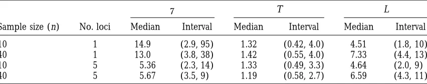
Inferences foru, T, and L from a single tree
u T L
Sample size (n) No. loci Median Interval Median Interval Median Interval
10 1 14.9 (2.9, 95) 1.32 (0.42, 4.0) 4.51 (1.8, 10)
40 1 13.0 (3.8, 38) 1.42 (0.55, 4.0) 7.33 (4.4, 13)
10 5 5.36 (2.3, 14) 1.33 (0.49, 3.3) 4.64 (2.0, 9)
40 5 5.67 (3.5, 9) 1.19 (0.58, 2.7) 6.59 (4.3, 11)
Median and 95% equal-tailed intervals of the posterior distributions foru 52Nm, tree height T, and total branch length L, based on samples of size n510, shown at the terminal nodes of the true tree of Figure 2, and n5 40 (not shown). The values of T and L are given in coalescent units; to obtain years, multiply by population size and generation time. The values used to generate the data were:u 55, T51.25, L54.82 (n5 10), and L57.15 (n540). Table entries are estimated from 10,000 output values (corresponding to 2 3 105attempts to update N andmand 1.63107branch-swapping steps); simulation error isz1–3% of stated
values.
tion is shown against each tree. Not surprisingly, the part of the Y chromosome. The true tree of Figure 2 is the same as that of Figure 1 (N.B. different time scale), simulated trees bear little resemblance to the true tree:
there is not enough information at a single microsatel- but in addition to the allelic data of Figure 1, a further four independent simulations of the ladder mutation lite locus to reconstruct the tree with any accuracy when
uis unknown. process are given, each with u 5 5. This simulation
mimics data from five completely linked microsatellite More detailed information about the inferences for
u, T, and L that can be drawn from the data is provided loci with a common value of u. Once again, four trees are shown simulated from the coalescent based on the by the first row of Table 1, which gives the postdata
median and 95% probability intervals for these parame- five-locus data, with a completely flat predata distribu-tion foru.
ters. The accuracy of inferences aboutu is very poor,
with a 95% interval of (2.9, 95), compared with a true As expected, the trees simulated from the postdata coalescent are, with information from l55 loci, more value of 5. At first sight, the situation looks better for
T: the median height of postdata trees is 1.32, close to similar to the original tree than in the one-locus case. Nevertheless, none of the simulations comes close to the correct value of 1.25. However, the 95% interval is
wide: (0.42, 4.0). Moreover, the 95% interval for the reconstructing the original tree.
Summary statistics for the n 5 10, l 5 5, case are height of the predata coalescent with n5 10 is (0.50,
4.5), so that the postdata 95% interval for T is not much given in row 3 of Table 1. Even with five loci, the post data uncertainty about T and L remain large, although narrower than the corresponding predata interval.
Simi-larly for L, the postdata 95% interval is (1.8, 10), com- inference about u is now much improved. Row 4 of Table 1 quantifies a further improvement when n is pared with a predata interval of (2.2, 12).
The effect of sample size: The true tree of Figure 1 is a increased to 40 (allelic data not shown).
Average performance over many trees: Each row of sub-tree of a tree with n540 terminal nodes (full tree
not shown). The height T of the full tree is 1.25, the Table 1 corresponds to only one realization of a genea-logical tree and allelic data. To obtain a better overall same as that for the n 5 10 sub-tree, but L is now
increased to 7.15. The second row of Table 1 summa- appreciation of the quality of inference achievable from microsatellite data, it is useful to assess average perfor-rizes the quality of inference attainable from the larger
sample size. For u, the width of the 95% interval has mance over many tree and mutation simulations. Care is needed to effectively summarize such a large quantity decreased substantially from 92 to 34. However, there
has been only slight improvement in inference about of simulation results, in part because the uncertainty in inference about u, T, and L tends to increase with the T and L. This may be because the additional data convey
information primarily about the part of the tree near magnitude of the true value.
For each ofu, T, and L, Figure 3 shows both the mean the terminal nodes, rather than near the root.
The effect of additional, linked loci: We have seen that absolute deviation (MAD) of the MCMC output values from the true value, and the length of the 95% probabil-there is only limited information aboutu, T, and L at
a single microsatellite, even when the modeling assump- ity interval (PIL) calculated from the MCMC run. For each combination of u, n and l, the height of the bar tions hold exactly. But is it perhaps possible to obtain
uncertainty, expressed as a proportion of the true length, tend to decrease with increasing n.
A limited number of simulations were performed with n5 200, l5 5, andu 5 5. Confidence inuincreased slightly with average values of MAD and PIL decreasing to 0.18 and 0.60, respectively. Only slight improvements to inferences on T were observed, but the precision of L increased further with n5200, giving a MAD of 0.19 and a PIL of 0.70.
Human Y chromosome microsatellite data: Human mitochondrial DNA sequences have been interpreted as supporting the theory—dubbed “Out of Africa”—that modern humans are descendants of a small group that lived in Africa perhaps about 200,000 years ago and subsequently spread throughout the world, eliminating most or all other extant human lineages. However, infer-ences about the time since the most r ecent common a ncestor (TMRCA) of the sample generally underesti-mate the amount of variability (Tavare´et al. 1997), and
geographical location of the MRCA is problematic and contentious (Templeton1993).
Patterns observed from autosomal DNA seem some-what different. For example, b-globin data suggest a much longer TMRCA (Harding et al. 1997). These
differing interpretations are not necessarily in conflict because autosomal and mitochondrial DNA reflect dif-ferent aspects of human history, and the results may be affected by selection effects. Recombination of autoso-mal DNA sequences may also lead to some problems
Figure2.—The true tree (top) is the same as that of Figure
for inference. 1, but the results of four additional, independent simulations
A third potential source of evidence, reflecting a fur-of the mutation process are also shown, mimicking data from
ther aspect of human prehistory, comes from genetic five completely linked loci, each having the same mutation
mechanism and withu 55. The other four trees are simulated variation on the human Y chromosome. Recently, a from the postdata distribution given all five data sets. These number of polymorphic microsatellites have become trees are samples numbered 2000, 4000, 6000, and 8000 from
available for population surveys (Cooper et al. 1996;
the MCMC run corresponding to row 3 of Table 1.
Dekaet al. 1996;Ruiz Linareset al. 1996; Hammeret
al. 1997;Zerjalet al. 1997).
A large effort has been concentrated on estimating expressed as a proportion of the true value. Inz5% of
MCMC runs, the value ofulay outside the 95% probabil- the TMRCA of a sample of genes drawn from a locus—in this case the entire nonrecombining portion of the hu-ity interval, and similarly for T and L, suggesting that
the MCMC runs had adequately converged. man Y chromosome. While the TMRCA may not be the most important time of human history (Brookfield
The poor quality of inferences about u when l 51,
noted for the particular tree of Figure 1, remains evident 1997), it is central to interpreting genetic samples and has been investigated by several authors (Goldsteinet
on averaging over many trees, especially for n510. In
the latter case the MAD of u is 3 to 5 times the true al. 1996;Tavare´et al. 1997). Furthermore, the method
proposed here allows simultaneous inferences about the value and the PIL as much as 20 times the true value.
Inferences become somewhat more precise as u in- TMRCA (the height of the tree) and, for example, the (effective) population size, N.
creases and markedly better as n and l increase.
Increases in n and l are less effective in improving Data: We consider the data ofCooperet al. (1996),
which consist of the genotypes of 212 individuals at the precision of T, with the improvement from worst
to best cases onlyz20% for both MAD and PIL when five Y chromosome microsatellite loci from East Anglia (UK), Sardinia, and Nigeria, together with a linked Alu
u 5 1, rising to 30% for larger values ofu. The same
patterns are shown as for u, with precision increasing insert. Since we are concerned here with inference from microsatellite haplotypes, we did not include the Alu with u, n, and l. Inferences about L are harder to
inter-pret because the true value increases with n. In the pre- insert in our analyses, although it could readily have been incorporated by means of a further augmentation data coalescent, the standard deviation of L decreases
Figure3.—Average mean
absolute deviation (MAD), left, and probability interval length (PIL), right, for u (top), T (middle), and L (bottom), each scaled by their respective true values. All values are averages over MCMC-generated samples of size 1000 (i.e., 1.63106
branch-swapping steps) from each of 140 datasets simu-lated under the coalescent-with-ladder-mutation model. Bars correspond to single locus with sample size of 10 (white) and 40 (light gray), and five linked loci with a sample size of 10 (dark gray) and 40 (black).
Two datasets were used: the complete set of Nigerian Priors: Under the standard coalescent, no information about the values N and m can be obtained from the and Sardinian haplotypes, together with the initial
sam-ple of 22 East Anglians (dataset NSE), and all 174 East allelic data except through their product, u 5 2Nm. Postdata inferences aboutuare therefore more robust Anglian haplotypes (dataset EA). The first of these sets
gives approximately equal weighting to the three re- than inferences about either N or m separately. It is useful to distinguish the two because information about gions; the second provides a larger sample from a single
location. Although the coalescent-with-ladder-mutation them can be obtained from other sources, particularly in the case ofm.Heyeret al. (1997) used three observed
model is unlikely to be exactly appropriate for these
datasets, inferences based on this model can neverthe- mutations in 1491 meioses to obtain a point estimate of mutation rate of 0.2% per meiosis. Assuming a Poisson less be informative. It is of particular interest to see what
such attempts between samples. After discarding the first 2000 samples (the burn-in), 10,000 samples were retained. Two such sets of samples were taken, with different starting trees, for each prior and dataset combi-nation. The posterior distributions form, N, T, and L approximated from the two MCMC runs were checked and in each case found to be effectively indistinguish-able. They were then combined to give a total of 20,000 samples.
Results are given in Figure 4 (probability density curves for dataset NSE; those for dataset EA are very similar and are not shown) and Table 2 (summary statis-tics for both datasets). For dataset NSE, a number of individual trees sampled from the MCMC output were examined in detail. Although there was some relation between geographic location of haplotype and tree structure, this was restricted to recent nodes. Clades of more than six haplotypes all from a single location were rare, and haplotypes from all locations were typically represented on both sides of the root node.
Inferences aboutu: Figure 4 (top right) shows, for data-set NSE, the two postdata probability density curves for
u 5 2Nm, as well as the corresponding predata curves. The postdata curves are very similar, despite the differ-ences in the two priors. For example, the postdata medi-ans are both around 11, compared with prior medimedi-ans of around 22 and 39, respectively, for the low- and high-variance priors (Table 2). Moreover, the two postdata
Figure4.—Posterior density curves for NSE data, together 95% probability intervals are practically
indistinguish-with corresponding prior density curves. See Table 2 legend able: (7.7, 17.0) and (7.6, 16.4). For dataset EA, the for details of data and prior distributions. The prior formis postdata medians and upper 95% interval limit are both shown as the dotted line in the top left. Elsewhere, the dotted
a little lower (Table 2). line and the dotted and dashed line correspond to the
low-As expected, the postdata distributions for the two and high-variance priors for N, respectively. Solid and dashed
lines show the postdata probability density assuming the low- components ofu, the mutation rate,m, and the popula-and high-variance priors, respectively. All postdata densities tion size, N, are negatively correlated, and each is more
are based on 20,000 output values. strongly affected by the prior than is the postdata
distri-bution ofu. Figure 4 (top left) shows the two post-NSE-data density curves for m, together with the predata based on these data, which we implemented as the prior curves. Both posterior curves are somewhat sharper than distribution for our analyses, is gamma with mode the prior, with diminished support for high values of 3/1492 and mean 4/1492. Inferences about the TMRCA m. The postdata density curves for N (Figure 4, bottom are insensitive to this assumption: a uniform prior for left) are very similar, despite the substantial difference
mleads to very similar conclusions (results not shown). in the prior curves. The post-EA-data distributions are
Tavare´ et al. (1997) used two prior distributions for
very similar to those for NSE. In all cases they reflect N: a gamma with mean 5000 and shape parameter 5, diminished support for high values of N. The postdata and a lognormal with parameters 9 and 1. Both these medians are z3000, with most likely values between distributions are centered at roughly 5000 individuals, z1500 and 8000 for both datasets. Although the limita-but the gamma is concentrated between z1000 and tions of the modeling assumptions require that caution 10,000, whereas the lognormal is more diffuse and posi- be attached to the interpretation of a particular analysis, tively skew, giving some support to values in excess of the similarity of the postdata distributions provides some 20,000. We also adopt these predata distributions for confidence for the conclusion that the Y chromosome N, referring to them (as well as the implied priors for effective population size during recent human history
u and the TMRCA) as the “low-variance” and “high- is a few thousands, consistent with the results of previous
variance” priors, respectively. analyses.
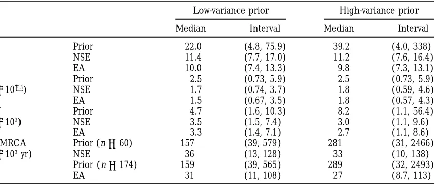
TABLE 2
Summary of human Y chromosome analyses
Low-variance prior High-variance prior
Median Interval Median Interval
u Prior 22.0 (4.8, 75.9) 39.2 (4.0, 338)
NSE 11.4 (7.7, 17.0) 11.2 (7.6, 16.4)
EA 10.0 (7.4, 13.3) 9.8 (7.3, 13.1)
m Prior 2.5 (0.73, 5.9) 2.5 (0.73, 5.9)
(31023) NSE 1.7 (0.74, 3.7) 1.8 (0.59, 4.6)
EA 1.5 (0.67, 3.5) 1.8 (0.57, 4.3)
N Prior 4.7 (1.6, 10.3) 8.2 (1.1, 56.4)
(3103) NSE 3.5 (1.5, 7.4) 3.0 (1.1, 9.6)
EA 3.3 (1.4, 7.1) 2.7 (1.1, 8.6)
TMRCA Prior (n560) 157 (39, 579) 281 (31, 2466)
(3103yr) NSE 36 (13, 128) 33 (10, 138)
Prior (n5174) 159 (39, 565) 289 (32, 2493)
EA 31 (11, 108) 27 (8.7, 113)
Median and 95% equal-tailed intervals of prior and posterior distributions foru,mN, and TMRCA for the
NSE sample (60 Y chromosome haploptyes, approximately equal numbers from Nigeria, Sardinia, and East Anglia), and for the EA sample (174 East Anglian haplotypes). Haplotypes consist of five microsatellite loci; data fromCooperet al. (1996). Prior distributions are:m zgamma (4,1492); Nzgamma (5,1/1000) (low
variance), and Nzln (9,1) (high variance). Table entries are based on 10,000 output values (corresponding to 43107branch-swapping steps).
N and T. Further multiplication by the generation time which opens up possibilities for inferences much more detailed than those previously possible. For example, G gives a posterior density curve for the number of years
since the MRCA. Figure 4 (bottom right) shows both the implications of the data for the scaled mutation parameter,u, and the height and shape of the genealogi-the pre- and post-NSE-data density curves, assuming G5
20. This value allows comparison with the results of cal tree can be assessed simultaneously. One key feature of our direct probability analysis is that likelihood
cal-Tavare´ et al. (1997), but may be too low: alternative
values can be implemented simply by proportional culations are greatly simplified by augmenting the parameter space to include the internal allelic states. adjustment.
The two postdata curves are very similar and reflect This innovation permits great flexibility in algorithms for exploring the space of possible trees, as well as in a very marked shift of support toward smaller values
compared with the predata distributions. For example, the range of modeling assumptions that become practi-cable. Here, we have focused on perhaps the simplest, the postdata distributions are sharply peaked at values
ofz30 kyr, a value that has little a priori support. Most plausible modeling framework: the coalescent-with-lad-der-mutation.
likely postdata values are between z10 and 100 kyr,
while values .150 kyr have probabilities of z1.5 and Results from simulation studies, in which the model-ing assumptions are known to hold exactly, indicate that 2% for the low- and high-variance priors, respectively.
For the much larger EA sample, drawn from a single accurate inference about u requires sampling several, tightly linked loci: a single locus provides little informa-geographic location, postdata distributions are shifted
slightly downward compared with the post-NSE-data dis- tion, even when the sample size is large. With five loci, good quality inferences about u are achievable, but tributions (Table 2).
The posterior distributions for (scaled) tree height, those for other aspects of the tree, such as T and L, remain far from precise.
T, have medians of z0.7 in all cases compared with
prior medians of z1.7. The scaled lengths, L, are not Turning to analyses of published data, although our modeling assumptions are, inevitably, not fully realistic, reduced to the same extent. This may be evidence for
“radial”-type trees, suggesting some recent population our results provide support both for an effective popula-growth. Nevertheless, the posterior values are also con- tion size of human Y chromosomes in the low thousands sistent with the standard coalescent model. and for relatively short times (point estimates around 30 kyr) since the most recent common ancestor. These conclusions in turn support the theory that extant hu-DISCUSSION
man males have spread relatively recently from a small group. In addition, the relatively small value for effective We have developed a methodology for carrying out
in reproductive success. The range of supported values attainable from the data are apparent from the simpler analyses presented here.
for u isz8 to 16. Improved predata estimates for the
mutation ratemwould enable more accurate inference We thankMark Beaumont, Richard Nichols,andBill Amos about the population size N and the TMRCA. Inferences for helpful discussions and comments, and the latter also for drawing our attention to the dataset. This work was supported in part by
from the two datasets were very similar, despite the fact
the Stochastic Modeling in Science and Technology initiative of the
that one was geographically dispersed and the other
United Kingdom Engineering and Physical Sciences Research Council
geographically homogeneous and much larger.
Addi-(Grant no. K72599).
tionally, there is little evidence of “clumping” of haplo-types from the same region, except in the very recent past from posterior trees.
LITERATURE CITED Values of the TMRCA supported by our analyses are
low compared both with times suggested by nongenetic Besag, J., P. Green, D. HigdonandK. Mengersen,1995 Bayesian evidence and with published studies based on autosomal computation and stochastic systems. Stat. Sci. 10: 3–66.
Best, N. G., M. K. CowlesandS. K. Vines,1995 CODA Manual DNA and mitochondria (Templeton1993;Hardinget
version 0.30. MRC Biostatistics Unit, Cambridge, UK.
al. 1997). They are, however, broadly consistent with the Brookfield, J. F. Y.,1997 Importance of ancestral DNA ages. Nature analysis ofTavare´et al. (1997), based on Y chromosome 388:134.
Brooks,S. P., 1998 Markov chain Monte Carlo method and its sequence data and the coalescent-with-infinite-sites
application. Statistician 47: 69–100.
model. [Our 95% intervals are narrower than those of Cooper, G., W. Amos, D. HoffmanandD. C. Rubinsztein, 1996
Tavare´et al. (1997), reflecting more information from Network analysis of human Y microsatellite haplotypes. Hum.
Mol. Genet. 5: 1759–1766.
five microsatellites than from .15 kb of sequence,
de-Deka, R., L. Jin, M. D. Shriver, L. M. Yu, N. Sahaet al., 1996 Disper-spite the limitations imposed by recurrent mutations.] sion of human Y-chromosome haplotypes based on five micro-Wide variation between Y chromosome, mtDNA, and satellites in global populations. Genome Res. 6: 1177–1184.
Di Rienzo, A., A. C. Peterson, J. C. Garza, A. M. Valdes, M. Slatkin autosomal TMRCAs are plausible for purely stochastic
et al., 1994 Mutational processes of simple-sequence repeat loci
reasons. Additional factors not accounted for in the in human populations. Proc. Natl. Acad. Sci. USA 91: 3166–3170. model may also explain the difference: male generation Di Rienzo, A., P. Donnelly, C. Toomajian, B. Sisk, A. Hillet al.,
1998 Heterogeneity of microsatellite mutations within and
be-time may be greater than female, and selective sweeps
tween loci, and implications for human demographic histories.
may play a large part in Y chromosome evolution.
Genetics 148: 1269–1284.
Our analyses were based on males from three loca- Donnelly, P.,1996 Interpreting genetic variability: the effects of
shared evolutionary history, pp. 25–50 in Variation in the Human
tions and may not represent all human Y chromosome
Genome, edited byK. Weiss.Wiley, Chichester, UK. history. Cooper et al. (1996) estimated the timing of
Donnelly, P.,andS. Tavare´ ,1995 Coalescents and genealogical population splits using a maximum divergence ap- structure under neutrality. Annu. Rev. Genet. 29: 410–421.
Dover, G.,1996 Slippery DNA runs on and on and on . . . Nat. proach. This gives an estimate of mT, where T is the
Genet. 10: 254–256.
TMRCA in generations. Their estimates ofmT were 11.4
Felsenstein, J.,1981 Evolutionary trees from DNA sequences: a for the whole data set and 7.75 for EA. These give point maximum likelihood approach. J. Mol. Evol. 17: 368–376. estimates for the TMRCA of 110 kyr for the whole data- Felsenstein, J.,1992 Estimating effective population size from
sam-ples of sequences: a bootstrap Monte Carlo integration method.
set and 77 kyr for the EA dataset. Estimates of
uncer-Genet. Res. 60: 209–220.
tainty are not available with this method. These values Fullerton, S. M., R. M. Harding, A. J. BoyceandJ. B. Clegg,1994 are toward the upper tails of our corresponding poste- Molecular and population genetic analysis of allelic sequence diversity at the humanb-globin locus. Proc. Natl. Acad. Sci. USA
rior distributions. Further, under our analyses the data
91:1805–1809.
suggest values for the TMRCA for the EA sample only Goldstein, D. B.,L. A. Zhivotovsky,K. Nayar, A. R. Linares, slightly lower than those for the NSE sample. They also L. L. Cavalli-Sforzaet al., 1996 Statistical properties of the
variation at linked microsatellite loci: implications for the history
suggest little increase in inferential precision with
in-of human Y chromosomes. Mol. Biol. Evol. 13: 1213–1218.
creasing sample size, in contrast to the conclusions of Gradshteyn, I. S.,andI. M Ryzhik,1980 Table of Integrals, Series, the original authors. and Products, Ed. 6. Academic Press, London.
Griffiths, R. C.,andS. Tavare´ ,1994 Ancestral inference in popula-Producing the first row of Table 1 required about
tion genetics. Stat. Sci. 9: 307–319.
about 50 min on a desktop workstation—equivalent to Hammer, M. F.,1995 A recent common ancestry for human Y chro-320,000 attempted tree rearrangements and 16,000 at- mosomes. Nature 378: 376–378.
Hammer, M. F., A. B. Spurdle, T. Karafet, M. R. Bonner, E. T. tempted changes touper minute. Increasing the sample
Woodet al., 1997 The geographic distribution of human Y size and number of loci increases the time required. To chromosome variation. Genetics 145: 787–805.
perform the same number of steps on a tree with five loci Harding, R. M., S. M. Fullerton, R. C. GriffithsandJ. B. Clegg,
1997 A gene tree for beta-globin sequences from Melanesia. J.
and a sample size of 200 takesz400 min. Computational
Mol. Evol. 44: s133–s138.
resources should not provide a barrier to extending our
Hastings, W. K.,1970 Monte Carlo sampling methods using Markov analyses to incorporate more sophisticated modeling chains and their applications. Biometrika 57: 97–109.
Heyer, E., J. Puymirat, P. Dieltjes, E. BakkerandP. De Knijff, assumptions. These might include more detailed
mod-1997 Estimating Y chromosome specific microsatellite mutation
els for population growth and structure and for
microsa-frequencies using deep rooting pedigrees. Hum. Mol. Genet. 6:
tellite mutation. Although such developments are well 799–803.
pp. 1–44 in Oxford Surveys in Evolutionary Biology, edited byD. J. al., 1996 Microsatellite evolution—evidence for directionality
and variation in rate between species. Nat. Genet. 10: 337–343.
FutuyamaandJ. Antonovics.Oxford University Press, Oxford.
Jarne, P.,andP. J. L. Lagoda,1996 Microsatellites, from molecules Ruiz Linares, A., K. Nayar, D. B. Goldstein, J. M. Hebert, M. T. Seielstadet al., 1996 Geographic clustering of human
to populations and back. Trends Ecol. Evol. 11: 424–429.
Kingman, J. F. C.,1982 The coalescent. Stoch. Proc. Appl. 13: 235– Y-chromosome haplotypes. Ann. Hum. Genet. 60: 401–408. Shriver, M. D., L. Jin, R. ChakrabortyandE. Boerwinkle,1993
248.
Kuhner,M. K., J. Yamato andJ. Felsenstein, 1995 Estimating VNTR allele frequency distributions under the stepwise mutation
model: a computer simulation approach. Genetics 134: 983–993. effective population size from sequence data using
Metropolis-Hastings sampling. Genetics 140: 1421–1430. Slatkin, M.,1995 A measure of population subdivision based on
microsatellite allele frequencies. Genetics 139: 457–462.
Levinson, G.,andG. A. Gutman,1987 Slipped-strand mispairing:
a major mechanism for DNA sequence evolution. Mol. Biol. Evol. Tavare´ , S., D. J. Balding, R. C. GriffithsandP. Donnelly,1997
Inferring coalescence times from DNA sequence data. Genetics
4:203–221.
Metropolis,N., A. W. Rosenbluth, M. N. Rosenbluth, A. H. 145:505–518.
Templeton, A. R.,1993 The “Eve” hypotheses: a genetic critique and TellerandE. Teller,1953 Equations of state calculations by
fast computing machine. J. Chem. Phys. 21: 1087–1091. reanalysis. Am. Anthropol. 95: 51–72.
Nei, M.,1987 Molecular Evolutionary Genetics. Columbia University Valdes, A. M., M. SlatkinandN. B. Friemer,1993 Allele
frequen-Press, New York. cies at microsatellite loci: the stepwise mutation model revisited.
Nielsen, R.,1997 A likelihood approach to population samples of Genetics 133: 737–749.
microsatellite alleles. Genetics 146: 711–716. Weber, J. L.,andC. Wong,1993 Mutation of human short tandem
Ohta, T.,andM. Kimura,1973 A model of mutation appropriate repeats. Hum. Mol. Genet. 8: 1123–1128.
to estimate the number of electrophoretically detectable alleles Zerjal, T., B. Dashnyam, A. Pandya, M. Kayser, L. Roeweret al.,
in a finite population. Genet. Res. 22: 201–204. 1997 Genetic relationships of Asians and Northern Europeans,
Press, W. H., S. A. Teukolsky, W. T. VetterlingandB. P. Flannery, revealed by Y-chromosomal DNA analysis. Am. J. Hum. Genet.
1992 Numerical Recipes in C, Ed. 2, Cambridge University Press, 60:1174–1183. Cambridge, UK.