Transactions of the 17th International Conference on
Structural Mechanics in Reactor Technology (SMiRT 17)
Prague, Czech Republic, August 17 –22, 2003
Paper # J01-5
Static Responses of Elasto –plastic Nonuniform Plates of Arbitrary
Shape
Dr.Subhash Chanda,
Deptt. of physics, A.C College, Jalpaiguri, West Bengal , India
Abstract: A simple method for the analysis of the elasto-plastic plates of arbitrary shape of
nonuniform thickness is developed. The method is based on the concept of isodeflectioncontour lines in
conjunction with Ilyushin
′
s theory for small plastic deformation. The method is applied to study the
nonlinear behaviour of circular and elliptical plates and the results obtained are compared with the
available results for structures of uniform thickness.
I N T R O D U C T I O N
Beyond elastic limit every elastic material exhibits plastic behaviour. For large amplitude vibration of structure under dynamic load and for a large flexure under static extreme load both elastic and plastic behaviour of substances are to be taken into consideration. Thin plates of arbitrary shape have a great practical importance in many engineering fields. The applications of nonuniform plates in mechanical engineering specially in aerospace engineering are very wide. However,the analysis of such structures appears to be quite difficult to yield adequately satisfactory results. Several approximate methods are in use for the analysis of such problems but these are restricted mainly to uniform structures having uniform thickness and of uniform flexural rigidity. The method of constant deflection contour lines have been used by different authors [1—6] to study the behaviours of plates and shells having uniform thickness and rigidity.The present paper aims at extending the method of constant deflection contour lines to study the nonuniform plate problems. The bending of an elliptic plate of elasto-plastic material with uniaxially varying thickness has been considered. The results obtained are presented in graphs and those are compared as far as possible with
DERIVATION OF BASIC DIFFERENTIAL EQUATIONS
A thin elasto-plastic plate of variable thickness and of variable flexural rigidity subjected to a continually distributed lateral load q(x,y) is considered. The middle surface of the plate remains in the x-y plane whereas the z-axis is perpendicular to that plane along the direction of centre of curvature. The intersections between the deflected surface z = w (x,y) and the planes z = constant yield contours which after projection onto z = 0 surface are the level curves called “ Lines of isodeflection“.The family of such curves is denoted by u(x,y) = constant. If the boundary of the plate is subjected to any combination of clamping and of simply support, then clearly it will belong to the family of lines of equal deflection and without loss of generality one may consider that u = 0 on the boundary of the plate. Denoting the family of curves u = constant by Cu, 0≤u≤u*, it is clear that Co = C is the boundary of the plate. It has been assumed that the value of `u `
increases as one moves towards the centre of the plate.
Considering the eqillibrium of an element Ω of the plate bounded by any closed contour Cu as shown in figure 2. Equating
the total downward load acting on an element to the resultant tractions exerted on this portion by the remainder of the plate,one obtains
∫ Vn ds = ∫∫ q dx dy...(1)
where the transverse reaction forces .
Vn = Qn - ∂/∂s( Mnt )...(2)
represents the effect of the shearing force Qn and the edge-rate of change of twisting moment Mnt along the contour Cu.
According to Ilyushin`s theory of the elastic plastic deformation (1948), the bending moments Mx,My,Mxy and their shear
forces Qx,Qy aregiven by the following relations:
X
Contour lines
Mx = - D ( 1 – ν ) { (∂2w/∂x2) + ν (∂2w/∂y2)}
My = - D ( 1 – ν ) { (∂2w/∂y2) + ν (∂2w/∂ x2)}
O
Mxy = D ( 1 – ν ) ( 1 – Ω ) (∂2w / ∂x∂y )...(3 Z
Qx = (∂/∂x) { M y} – (∂/∂y) {Mxy}
Qy = (∂/∂y) { M x} – (∂/∂x) { M xy) }
Y Figure: 1
Where, Ω = 0 when e ≤ 1, the region is elastic ; when e > 1 the region is plastic. Also,
Ω = λ [ 1 – ( 3 / 2e ) + ( 1 /2e3 ) ]...(4)
and e2 = (h2/3e
s) [(∂2w/∂x2)+(∂2w/∂y2 )+(∂2w/∂x∂y)+(∂2w/∂x2) (∂2w/∂y2) ... (5)
in which es is the yield strain, ν is the poisson`s ratio, D is the flexural rigidity of the plate material, λ is a material
constant
The expressions for Qn , Mnt are well known and given by,
Qn = Qx Cosα + Qy Sinα
Mnt = Mxy ( Cos2 α - Sin2 α ) + (Mx -My) Sin α Cosα ...(6)
Where, Cosα = (dy / ds ) and Sinα = - ( dx / ds ) .
Making use of relations (3), (5) and carrying out several steps of computation equation (1) finally takes the form:
(∂ 3w/∂ u 3)) ∫ ( 1 – Ω) [ R + (3m/a) Rx + 3 (m/a) 2 Rx2 + (m/a)3 Rx3 ] ds
(∂ 2w/∂ u 2) ∫ ( 1 – Ω) [ F + (3m/a) Fx + 3 (m/a) 2 Fx2 + (m/a)3 Fx3 ] ds
(∂w/∂ u) ∫ ( 1 – Ω) [ G + (3m/a) Gx + 3 (m/a) (∂u/∂x ) + (m/a)3 Fx3 ] ds
(∂ 2w/∂ u 2) ∫ D [ (∂Ω /∂x ) (∂u /∂x ) +(∂Ω /∂y ) )(∂u /∂y ) ] √ t ds +
(∂w/∂ u) ∫( D/√ t ) [(∂Ω /∂x ) K +(∂Ω /∂y) L ] ds - ∫ (∂D /∂x ) ( 1 – Ω) (∂2w/∂x2) + ν (∂2w/∂y2) ] ((dy / ds ) ds - ∫ (∂D /∂x ) ( 1 – Ω) ( 1 – ν )
(∂2w / ∂x∂y ) (dy / ds ) ds = ∫∫ q dx dy...(7)
where, t = u2
x + u2y , R = - D0 (√ t )3
F = -(D0/ √ t) [ 3 uxx ux2 +3 uyy uy2 + uxx uy2 + uyy ux2 + 4 uxy ux uy ]
G = --D0/ (√ t) 3[uxxx ux3 + uyyy uy3 + (2 - ν ) (uxxx ux uy2 + uyyy uy ux2 + uxyy ux3 +
uxxy uy3 )+ (2 ν – 1 ) (uxyy ux uy2 + uxxy uy ux2 ) - 2 ( 1 – ν ) (uxy uxx ux uy - uxy2
uy2- uxy2 ux2 + ux uy uxy2) + ( 1 – ν ) (uxx - uyy) (uxx ux2 - uyy ux2 )] +
2 D0( 1 – ν )/( √ t) 5[uxy(ux2 – uy2) - (uxx ux uy - uyy ux uy ) ]2
K = (uxx ux + ν uyy ux ) + [( 1 – ν ) uxy uy - uy( H/D) ],
L = uy (uyy + ν uxx ) + ux [ (1- ν) uxy + H/D ],
H /D = (1- ν)/t [uxy ( u2x - u2y ) – ux uy ( uxx - u yy ) ]
h = ho ( 1 + mx/a ), D = DO ( 1+ mx/a )3 , Do = Eho3/ 12 (1- ν2) ...(7)
In the elastic region where Ω is identically Zero and for a plate of uniform thickness ( m = 0), equation (6) reduces to the usual ordinary differential equation.
In the elastic region and plastic region e2 is given by
e2 = ( h
o / 3es2 ) [ M W,2u + N W,u W,un + t2 W,2un ] ...(9)
Where M = ( 1 + mx/a )2 [ u2
xx + u2yy + uxx uyy + u2xy ]
N = ( 1 + mx/a )2 [ 2 u
xxu2x + 2 uyy u2y + uxxu2y +uyy u2x + 2uxy ux uy ] ...(10)
Consequently, whenever the contour lines u(x,y) = constant are known the problem reduces to the solutions of equations ( 8 ) and ( 9) with continuity of the solution at the boundary of the elastic and plastic regions.
It is to be noted that the precise form of isodeflection contour lines may be obtained in many cases by symmetry consideration or by intuition otherwise assumption may be made as a first approximation.
ILLUSTRATIONS
Uniformly loaded elliptic plate
For example, we consider the bending of a simply supported elliptic plate of variable thickness under uniformly distributed transverse load.
The frist approximtion to the lines of equal deflection for elastic case may reasonably be taken as
u ( x,y ) = 1- x2 /a2 - y2 / b2 ...(11)
where ‘a’ and ‘b’ are the semi major and minor axes of the ellipse respectively
Since Ω is a function of ‘e’ which in turn is a function of ‘u’ and considering the form of u given by equation (11) and carrying out the necessary calculations as explained by Mazumder (1970), the equation (6) takes the form :
( 1- u ) (1 – Ω ) w,uuu H1 – 2( 1- Ω ) H2 w, uu - ( 1 – u ) H1w,uu + H3 w,u Ω,u
+ ( 1 – Ω ) H4 = qa4 b4 /(2DOP* ) ...(12)
Where, P* = 3a4 + 2a2 b2 + 3b4
H1 = 1+ 16 m (1 + u ) 1/2 ( 3a4 + 4a2 b2 + 3b4 ) / ( 5 Пp * ) + 3m2 ( 1 - u ) (a4 + 2a2 b2 + 5b4 ) / ( 2p* )
+32m3 (1 - u) 3/2 ( a4 + a2 b2 + 8b4 ) / (35 П p * )
H2 = 1 + 6m (1 + u ) 1/2 ( a4 + 2a2 b2 + b4 ) / ( П p * ) + 3m2 ( 1 - u ) (3a4 + 4a2b2 + 9b4 ) / ( 4p* )
+8m3 (1 - u) 3/2 ( 3a4 + 5a2 b2 + 12b4 ) / (15 П p * )
H3 = [ { 2 + 8m (1 + u )1/2
+ 3m
2 ( 1 - u ) / 2 + 16m3 ( 1 - u ) 3/2 / 15 П } { (a / b ) ( ν / a2 + b2 )}+ { 2 + 32m ( 1 + u ) 3/2 / П + 9m2 ( 1 + u ) + 32m3 ( 1 – u ) 3/2 / 15 П )} {( b / a ) (1 / a2 + ν / b2)} a2 b3/p*
H4 = [ ( 1 / ab ) { 8m ν ( 1 – u )1/2 / ( П ) + 3m2 ν ( 1 - u ) + 16m3 ( 1 - u ) 3/2 / (5 П ) } + ( b / a3 )П
{ 16m (1 – u )1/2 / ( П ) + 9m2 ( 1 – u ) + 16m3 ( 1 - u ) 3/2 / ( 5 П ) } – ( b / a ) ( 1/a2 + ν/b2 ) { 12m ( 1-u )1/2/ ПW + 6m2 +
8m3 (1-u )1/2 / (П ) } ] ( a3 b3 / p* )
Using the following non dimensional parameters
W = wh 0 / esa2 ; Q = qa2ho / 2Does ; β= b4 / p*
Equation ( 12 ) reduces to
( 1 – u ) ( 1 – Ω ) H1 W,uuu - 2 ( 1 – Ω ) H2 W,uu - ( 1- u ) H1 Ω,u W,uu
H3 Ω, u W, u + ( 1 – Ω ) H4 = - βQ ...(13 )
and the expressions for e2 and Ω,
u are as follows :
e2 = ( a4/ 3 ) [ M W,2u + N W,u W,uu + t2 W,uu ] ...(14 )
Ω,u = P [ 2M W,u W,uu + N W,2uu + N W,u W,uuu + 2t2 W,uu W,uuu ] ...(15 )
The set of boundary conditions in nondimensional form are as follows:
W | = 0 , ( 1 - u ) W,uu - ( 1 + ν ) / 2 W,u | = 0, ( 1 – u ) W,u | = 0
|u=0 |u=0 |u=1...(16)
METHOD OF SOLUTION
The non linear governing differential equation (13) can be solved numerically using Finite difference and Range-kutta methods (BURDEN et al,1986). But here a completely new approach towards series solution for better approximation has been presented.
n
Let W = ∑ Aj u j ...(17)
J=3
The series starts at j = 3 as the approximate solution is to satisfy the boundary conditions. Substitution of the Σtrial solution in equation (13) yields the following residual:
n n n R1 = ( 1 - u ) k 1 H 1 ∑ j ( j – 1 ) ( j – 2 ) Aj u j-3 - 2 k 1 H 2
Σ
j ( j - 1 ) A j u j k 2 H 1 (1 - u )Σ
j =3 j=3 j=3
j ( j –1 ) A j u j –2 + k 2 H 3 Σ j A j u j –1 k 1 H 4 + β Q ...( 18)
where k 1 = ( 1 - Ω ) , k 2 = Ω, u
Also, the expressions for e 2 and Ω, u takes the forms:
n n n n e 2 = ( a 4 / 3 ) [ M { Σ j A
j u j-1 } 2 + N {Σ j A j u j –1 }{ Σ j (j –1 ) A j u j –2 } + t 2 { Σ j (j – 1)
j=3 j=3 j=3 j=3
A j u j-2 } 2...(19)
n n n
Ω,u = P [ 2 M { Σ j ( j - 1 ) A j u j - 2 } { Σ j A j u j – 1 } + N { Σ j ( j-1) A j u j –2 } 2
3 3 3
n n n n
+ N { Σ A j j u j –1 } { Σ Aj ( j – 1 ) ( j – 2 ) u j – 3 } + 2 t 2 {Σ A j u j – 2 j ( j- 1 )} {Σ A j u j – 3 j ( j-1) (j –2 )]
j=3 j=3 j=3 j=3
To find the coefficients A j for j = 3,4,5,...n, we solve the following sets of equations in accordance with Galerkin`s orthogonality procedure
1
∫ R 1 ( u ) du = 0 , j = 3,4,5,...n. ...(21) 0
It is necessary to find the average value of ` e ` and Ω, u over the domain of the ellipse given in equations
(11) if the equations in ( 21 ) are to be solved. As a demonstration of the solution for a simple but dominating case ( as it is converging) n=3 and n=4 are substituted into the above equations.
The results corresponding to (21) are as follows:
A 3 = --- ... (22)
308 K 12 - 8.96 K 1 K 2 + 3.2 K Q ( 1.55 k 2 - 4.8 k 1 ) A 4 --- ...(23)
( 308 K 12 - 8.96 K 1 K 2 + 3.2 K 22 The central deflections ( u = 1 ) for this case is W 0 = [( 0.2 Q - 0.001) / ( 18.8 - 2.7 Q ) ] 0.5 + [ ( 0.02 Q - 0.008 ) / ( 18.8 - 1.09 Q )] 0.5...(24)
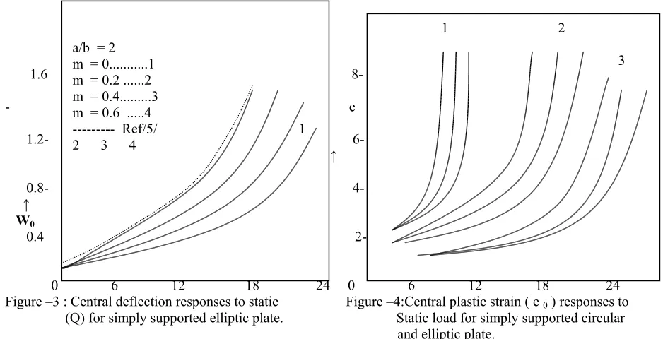
The numerical results for various aspect ratio ( R = a/b ) and the thickness variation parameter (m) are computed and shown in graphs ( 1 – 6 ). The results obtained using Runge-Kutta as well as Finite difference are in close agreement with the present results. Also, the results are in good agreement with those obtained by Mazumder for m = 0 .The present results exhibits little variation with the results of TIMOSHENKO & WOINOWSKY (1953) for higher values of `R`. For higher values of taper constant (m) the assumption of isodeflection contour lines may be a greater approximation for simply supported elliptic plate.
Observations and conclutions
In figure 1 , central deflection (W 0 ) responses to static load (Q) for simply supported circular plate has been shown and it is concluded that tha taper thickness has a considerable contributions to the static load which increases with the increase of the value of ` m `,the taper thickness. In figures 2 & 3 the same characteristics as in figure 1 have been drawn for an elliptic plate and it is observed that here also the required load for certain deflection increases with the increase in the value of ` m`. In figure 4, the central plastic strain (e 0 ) responses to static load for simply supported elliptic plate and circular plate have been drawn and found that in all cases central plastic strain increases with the increase of the value of ` m`. In figures 5 & 6 the variation of plastic load with the changeover radius has been depicted and it isobserved that the taper thickness has great influence on the response and increases with the value of the changeover radius. From a literature survey it seems that the application of constant deflection contour lines method in I ii iiinonhomogeneous plastic plate is completely new. Though the validity of the method is long established till its application in solving nonuniform elastic and plastic plates and shells problems seem to be new. 1.6- 1.6 1.2- 1.2 W0 W0 0.8 0.8- 0.4- 0.4 0 0
- 0 3 6 9 12 0 6 12 18 24
a/b = 1.5 i ii iii iv
m = 0 ...i
m =0.2 ...ii
m = 0.4 ...iii
m = 0.6 ...iv
i ii iii iv a/b =1 m = 0 ...i
m = 0.2 ...ii
m = 0.4 ...iii
m = 0.6 ...iv
Q Q Figure - 1 Figure – 2
1.6 8-
- e 1.2- 6-
↑ e 0 0.8- 4-
↑ W0 0.4 2-
0 6 12 18 24 0 6 12 18 24
a/b = 2 m = 0...1
m = 0.2 ...2
m = 0.4...3
m = 0.6 ...4
--- Ref/5/ 1
2 3 4
1 2 3
Figure –3 : Central deflection responses to static Figure –4:Central plastic strain ( e 0 ) responses to (Q) for simply supported elliptic plate. Static load for simply supported circular and elliptic plate. 80 80
60 60
__ __ Q Q 40 40
20 20
0 0
REFERENCES
1 A.A. 1Ilyushin, 1948 OGIZ, GITTL, MOSCOW, Leningrad. Plastici
2. R.K.Jain and J. Mazumder, 1994 International Journal Of Plasticity, Vol. 10, 749 – 759. Research note on the elastic plastic bending of rectangular plates.
3 J.Mazumdar and D.Bucco, 1978 Journal Of Sound and Vibration, Vol. 57, 323 – 331. Ttransverse vibrations of viscoelastic shallow shells.
4. J.Mazumdar, Journal of Australian Mathematical Society,Vol. 11, 95 –112.Amethod for solving problems of elasticplates of arbitrary shape.
5. J.mazumdar and R.K.Jain, International Journal Of Plasticity, Vol.-5, 463 –475. Elastic Plastic analysis of plates of arbitrary shape- Anew approach.
6. R.Jones and J.Mazumdar, 1`974 Journal of Acoustical Society of America,Vol. 56, 1487 – 1492, Transverse vibrations of shallow shells by the method of constant deflection contours.
7. J.Mazumdar , 1971 JSV, Vol. 18,147 –155. Transverse vibrations of elastic plates by the method of constant deflection lines.
8. S.Chanda and M.M.Banerjee, , Belgium Society of Mechanical Engineering,European Journal, Vol. 4 ,pp 172 – 176 Large deflections of thin elastic plates of arbitrary shape placed on elastic foundation.