Semiparametric Efficient Estimation of Treatment Effect in a Pretest-Posttest Study with Missing Data

Abstract

LEON, SELENE REYES. Semiparametric Efficient Estimation of Treatment Effect in a Pretest-Posttest Study with Missing Data. (Under the direction of Anastasios A. Tsiatis and Marie Davidian.)

Inference on treatment effect in a pretest-posttest study is a routine objective in medicine, public health, and other fields, and a number of approaches have been advocated. Typically, subjects are randomized to two treatments, the response is measured at baseline and a prespecified follow-up time, and interest focuses on the effect of treatment on follow-up mean response. Covariate information at baseline and in the intervening period until follow-up may also be collected. Missing posttest response for some subjects is routine, and disregarding these missing cases can lead to biased and inefficient inference. Despite the widespread popularity of this design, a consensus on an appropriate method of analysis when no data are missing, let alone on an accepted practice for taking account of missing follow-up response, does not exist.

SEMIPARAMETRIC EFFICIENT ESTIMATION OF TREATMENT EFFECT IN A PRETEST-POSTTEST STUDY WITH MISSING DATA

by

SELENE LEON

A dissertation submitted to the Graduate Faculty of North Carolina State University

in partial fulfillment of the requirements for the Degree of

Doctor of Philosophy

STATISTICS

Raleigh

2003

APPROVED BY:

Anastasios Tsiatis Marie Davidian

Chair of Advisory Committee Chair of Advisory Committee

Biography

Acknowledgements

I am grateful to so many persons and organizations that enumerating them all would be another chapter of this dissertation. So, missing someone is just due to lack of space, not of memory.

The support and patience that my advisors, Dr. Tsiatis and Dr. Davidian, consis-tently showed during my doctoral research is an inspiration to continue their example, under a different context, in my professional development.

I am also grateful to all faculty members from the Statistics Department and other Departments for their willingness to provide skills that open opportunities to persons who consider that scientific knowledge is nowadays, a fundamental tool for professional development. I also truly appreciate the friendship, encouragement and moral support from all faculty, staff and students from NC State U.

I want to thank Michael Hughes, Heather Gorski, and the AIDS Clinical Trials Group for providing the data from ACTG 175.

I am also grateful for the economical support provided by the Graduate School, as well as the grants R01-CA51962, R01-CA085848, R01-AI31789 from the National Institutes of Health for my doctoral studies. I also want to thank GlaxoSmithKline Inc. for the opportunity to practice the skills and scientific knowledge acquired in school in an industrial context.

Contents

List of Figures vii

List of Tables ix

1 Introduction 1

2 MODEL 10

2.1 Full data model . . . 10

2.2 Observed data influence functions . . . 16

3 Practical Implementation 26

3.1 Full data . . . 26 3.2 Missing at random follow-up. . . 31 3.2.1 Estimators Based on a Restricted Class of Influence Functions 35

4 Simulation evidence 40

4.1 Full data. . . 40

5 Treatment effect in ACTG 175 57 5.1 20±5 CD4 . . . 57 5.2 96±5 CD4 . . . 58

6 Discussion 63

List of Figures

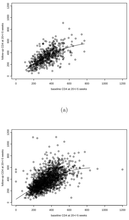
1.1 ACTG 175: CD4 counts after 20±5 weeks vs. baseline CD4 counts for patients randomly assigned to a. ZDV alone (“control”) and b. the combination of ZDV+ddI, ZDV+ddC, or ddI alone (“treatment”). The solid lines were obtained using the Splus functionloess()(Cleveland, Gross, and Shyu, 1993); inb., use of different span values and deletion of the apparent “high leverage” points with the largest baseline CD4 all lead to similar curvilinear fits. . . 8

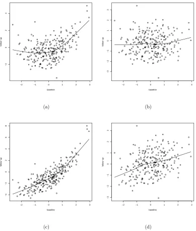
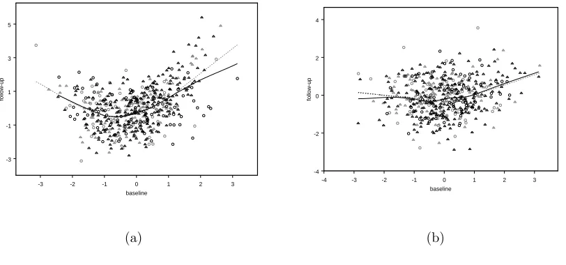
4.1 Simulated data for n = 500 from scenarios a. Q1 and b. based on (4.1.1) and scenarios c. N1 and d. N2 based on (4.1.2), with smooth fits (solid line) obtained using the Splus functionlowess()(Cleveland, 1979). Each panel depicts data for roughly 250 subjects randomized to control. . . 48 4.2 Simulated data for n = 1000 from scenarios a. Q1 and b. based

on (4.2.3) and scenarios c., with smooth fits obtained using the Splus functionloess()(Cleveland, 1979). Solid lines are fitted utilizing only complete cases (observations in black), in contrast, dotted lines are based on the “full” data, as if all observations were available (cases con-sidered as missing follow-up response are colored in light grey). Data represented with triangles are observations with intermediate bernoulli value X1 = 1. Each panel depicts data for roughly 500 subjects

List of Tables

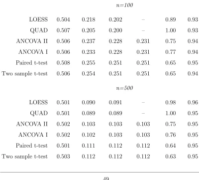
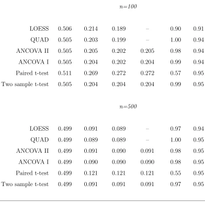
4.1 Simulation results for true quadratic relationship (4.1.1), 5000 Monte Carlo data sets. Estimators and scenarios are as described in the text. MC Mean is Monte Carlo average, MC SD is Monte Carlo standard de-viation, Asymp. SE is the average of estimated standard errors based on the asymptotic theory, OLS SE is the average of estimated stan-dard errors based on OLS for the “popular” estimators, MSE Ratio is Mean Square Error (MSE) for QUAD divided by MSE of the indicated estimator, CP is empirical coverage probability of confidence interval using asymptotic SEs. . . 49

4.2 Simulation results for true quadratic relationship (4.1.1), 5000 Monte Carlo data sets. Columns are as described in table 4.1. Estimators and scenarios are as described in the text. . . 50

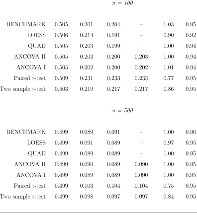
4.4 Simulation results for true nonlinear relationship (4.1.2), 5000 Monte Carlo data sets. Estimators and scenarios are as described in the text. Column headings are as in Table 4.1. . . 52

4.5 Empirical size and power of Wald tests (estimate/asymptotic standard error estimate) ofH0 :β = 0 under scenario N1 with (4.1.2), each based

on 5000 Monte Carlo data sets. Empirical size was found by simulations with β = 0. Empirical power is under the indicated alternative. . . . 53

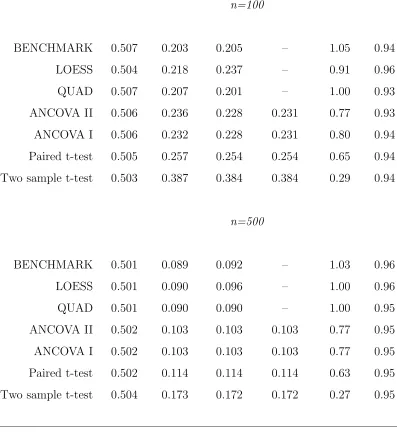
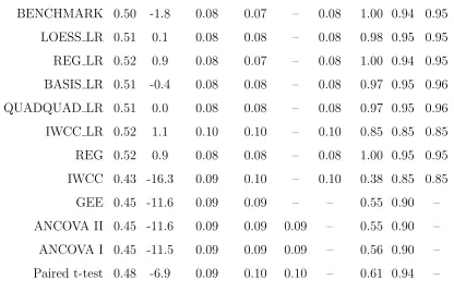
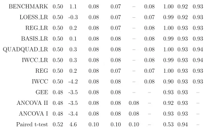
4.6 Simulation results for true quadratic relationship (4.2.3), 1000 Monte Carlo data sets with sample size ofn = 1000. Estimators and scenarios are as described in the text. Bias is the percent relative bias. Columns headings are as described in table 4.1. MSE Ratio is Mean Square Error (MSE) for BENCHMARK divided by MSE of the indicated esti-mator, CP and CPsw are empirical coverage probabilities of confidence interval using asymptotic and sandwich SEs respectively. Treatment effect parameter value is β = 0.51. . . 55

5.1 Treatment effect estimates for 20±5 week CD4 counts for ACTG 175. The methods are as denoted as in Tables 4.1-4.5; in addition, BASE-QUAD denotes the proposed basis function method including up to quadratic terms in baseline CD4 and linear terms involving baseline co-variates, and BASE-GAM denotes the proposed method estimating the conditional expectations using generalized additive models. Asymp-totic SE is estimated standard error based on the influence function and OLS SE is estimated standard error based on the “usual” ap-proaches for the “popular” estimators as described in Section 4. . . . 61 5.2 Treatment effect estimates for 96± 5 week CD4 counts for ACTG

Chapter 1

Introduction

The pretest-posttest trial is ubiquitous in research in medicine, public health, and numerous other felds. In the usual study, subjects are randomized to one of two treatments (e.g., treatment and control) and the response of interest is ascertained for each at baseline (pre-treatment) and follow-up. The objective is to evaluate whether treatment affects follow-up response, with baseline responses serving as a basis for comparison. For instance, in many HIV clinical trials, interest focuses on comparing treatment effects on viral load or CD4 count after a specified period, with baseline observations on these quantities routinely available.

treatment included as a covariates in a linear model, referred to by Yang and Tsiatis (2001) as ANCOVA I and ANCOVA II, respectively. A nonparametric approach in a different spirit was proposed by Quade (1982); we do not consider this here. The two-sample t-test seems predicated on the assumption that baseline and follow-up responses are uncorrelated, so that no precision is to be gained from incorporating baseline information, while the others (paired t-test and ANCOVA I and II) implicitly rely on an apparent assumption of linear dependence between follow-up and baseline response. All are often associated with the assumption of normality.

(2001) showed that all these estimators are consistent and asymptotically normal; the GEE estimator is asymptotically equivalent to that from ANCOVA II and most efficient; when the randomization probability is 0.5 or covariance between baseline and follow-up responses is the same for both treatment and control, the ANCOVA I estimator is asymptotically equivalent to ANCOVA II/GEE; and, if baseline and follow-up responses are uncorrelated, the two-sample t-test estimator achieves the same precision as ANCOVA II but is inefficient otherwise, while the paired t-test is equivalent to ANCOVA II only if the difference between follow-up and baseline is uncorrelated with baseline within each treatment.

As the ANCOVA approaches are derived from a supposed linear relationship be-tween baseline and follow-up, some practitioners are reluctant to use them; asymptotic equivalence of the GEE estimator indicates it involves the same considerations. Yang and Tsiatis (2001) showed that consistency and asymptotic normality hold even if linearity is violated. However, as their study restricted attention to such “linear” estimators, it did not address whether or how it might be possible to improve upon these approaches under deviations from linearity and without limiting distributional assumptions.

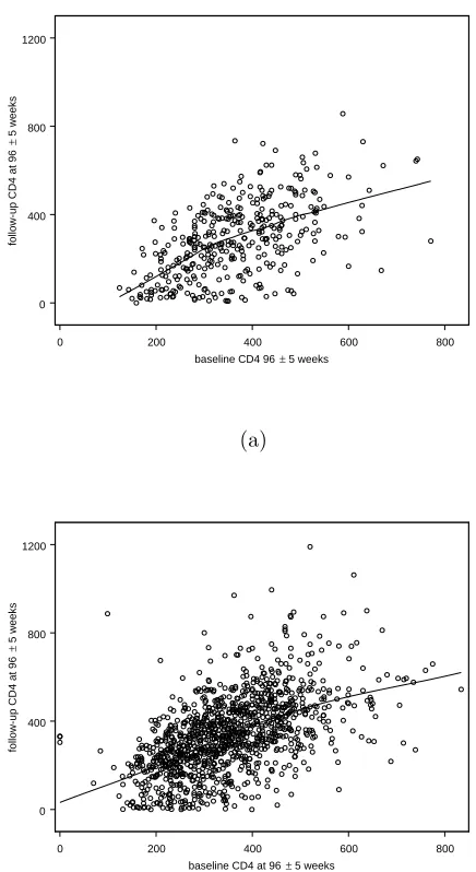
death showed ZDV to be inferior to the other three therapies, which showed no differ-ences. Figure 1.1 plots CD4 counts at 20±5 weeks, a follow-up measure that reflects early response to treatment subsequent to the often-observed initial rise in CD4 (e.g. Tsiatis, DeGruttola, and Wulfsohn, 1995), versus baseline CD4 for the ZDV-only (“control”) and other therapies combined (“treatment”) groups and suggests a possi-ble departure from a straight-line relationship. Figure 1.2, which plots CD4 counts at 96 ± 5 weeks, shows similar behavior. Indeed, nonlinear relationships are a routine feature of biological phenomena, as is nonnormality; histograms of CD4 counts at baseline and follow-up for each group (not shown) exhibit the usual asymmetry that motivates the standard analysis on the log, fourth-, or cube-root scale.

the assumption that follow-up is missing at random (MAR) (Rubin 1976), associ-ated only with these observable quantities and not the unobserved response, may be reasonable. Even if such a MAR mechanism may be postulated, valid methods to take appropriate account of missingness in pretest-posttest analysis have not been widely applied by practitioners, and, rather,ad hocapproaches such as complete-case analysis have been commonplace.

Semiparametric models, written in terms of a finite-dimensional parameter of in-terest and an unspecified infinite-dimensional component, have gained considerable popularity as they embody less restrictions (and thus fewer potentially incorrect as-sumptions) than fully parametric models. In a landmark paper, Robins, Rotnitzky, and Zhao (1994) derived an asymptotic theory of inference for general semiparamet-ric models with data MAR. Genesemiparamet-rically, for parameter β in a statistical model, an estimator βbbased on iid observations Wi, i = 1, . . . , n,is asymptotically linear with influence functionϕ(W) ifn1/2_{(βb−β) =n}−1/2Pn

i=1ϕ(Wi)+op(1) andE{ϕ(W)}= 0, E{ϕT_{(W)ϕ(W)}<∞; regular, asymptotically linear (RAL) estimators (Newey 1990)}

b

β are consistent and asymptotically normal under weak conditions with asymptotic variance E{ϕT_{(W)ϕ(W)}. Thus, by identifying all influence functions for a} partic-ular model, consistent estimators may be deduced. Robins et al. (1994) not only characterized the class of influence functions for all RAL estimators for the paramet-ric component of general semiparametparamet-ric models with data MAR, but also identified the efficient member of the class with smallest variance.

MAR data under specific distributional assumptions or adapt “popular” estimators such as ANCOVA to handle MAR on a case-by-case basis, a more broadly-applicable strategy is to take a semiparametric perspective and use this theory to elucidate a unified framework for pretest-posttest analysis. Interestingly, despite the ubiquity of the pretest-posttest study in numerous fields and the simplicity of the model when no data are missing, to our knowledge, explicit application of this pioneering theory to pretest-posttest inference with data MAR with an eye toward development of practical estimators on its basis and associated detailed study and illustration of performance of resulting techniques has not been reported.

A main objective of this dissertation is to develop practical strategies for esti-mation of β in a semiparametric pretest-posttest model from the perspective of the Robins et al. (1994) theory by indicating the class of influence functions for all RAL estimators for β when follow-up response is MAR, including the most efficient. We first apply this theory in this setting, using it to identify the class of all influence functions when no follow-up data are missing by casting the full-data situation as an “artificial” missing data problem by defining counterfactual follow-up responses (e.g. Holland 1986). A key finding is that the resulting estimators exploit the rela-tionship of baseline response and covariates to follow-up response in a way that leads to substantial efficiency gains over “popular” approaches such as ANCOVA or the paired t-test, which are revealed to yield inefficient members of the class of consistent estimators for β.

and covariates play a role in enhancing precision, demonstrate how the theory leads to practical estimators, and study the performance of such approaches.

baseline CD4 at 20+/-5 weeks

follow-up CD4 at 20+/-5 weeks

0 200 400 600 800 1000 1200

0

200

400

600

800

1000

1200

(a)

baseline CD4 at 20+/-5 weeks

follow-up CD4 at 20+/-5 weeks

0 200 400 600 800 1000 1200

0

200

400

600

800

1000

1200

(b)

0 200 400 600 800 baseline CD4 96 ± 5 weeks

0 400 800 1200

follow-up CD4 at 96

±

5 weeks

(a)

0 200 400 600 800 baseline CD4 at 96 ± 5 weeks

0 400 800 1200

follow-up CD4 at 96

±

5 weeks

(b)

Chapter 2

MODEL

2.1

Full data model

In this section, assume no missing follow-up and that each subject i= 1, . . . , nis randomized to treatment with known probability δ, so Zi = 0 or 1 as i is assigned to control or treatment, respectively. Let Y1i and Y2i be i’s observed baseline and follow-up responses, leading to observed data for i (Y1i, Y2i, Zi); the subscript i is suppressed when no ambiguity will result.

We develop the model by conceptualizing the situation in terms of counterfactuals or potential outcomes, a key device in the study of causal inference (e.g., Holland, 1986), and then expressing the observable data in terms of these quantities. The variablesY1 andZ represent phenomena prior to treatment action, while Y2 is a

set of counterfactual random variables (Y₂(0), Y₂(1)) is obviously not observable for any subject but rather represents what potentially might occur at follow-up under both treatments, including that “counter to the fact” of what might actually be assigned in the trial. We place no restrictions on the joint distribution of the counterfactuals and Y1, such as equal variance or independence, and define µ1 = E(Y1), σ11 = var(Y1);

for c = 0,1, µ(2c) = E(Y (c) 2 ), σ

(c)

22 = var(Y (c)

2 ); and σ (c)

12 = cov(Y1, Y2(c)). Thus, e.g.,

µ(0)₂ =E(Y₂(0)) denotes mean follow-up response if all subjects in the population were assigned to control. It is natural to assume that the observed follow-up response under the subject’s actual, assigned treatment corresponds to what potentially would be seen if the subject were assigned to that treatment; i.e., Y2 =Y2(0)(1−Z) +Y

(1) 2 Z.

The observed assignment Z is made at random, so without regard to baseline status or prognosis; thus, assume Z is independent of (Y1, Y2(0), Y

(1)

2 ). As usual, we assume

(Y1i, Y2(0)i , Y

(1)

2i , Zi) and hence (Y1i, Y2i, Zi) are independent and identically distributed (i.i.d.) across i.

Interest focuses on the difference in population mean follow-up response, which, under the usual causal inference perspective (Holland, 1986), may be thought of as the difference in means if all subjects in the population were assigned to control or treatment, respectively; i.e., β = µ(1)₂ −µ(0)₂ = E(Y₂(1))−E(Y₂(0)). Under our assumptions, in fact β = E(Y2|Z = 1)−E(Y2|Z = 0), the usual expression for the

difference of interest in a randomized trial; andE(Y2|Z) =µ2+βZ andE(Y1|Z) =µ1,

writingµ2 =µ(0)2 =E(Y (0)

2 ) for brevity.

means is that it reveals a structure analogous to that in missing data problems. As we are interested in the difference of the two marginal quantitiesµ(1)₂ andµ(0)₂ , we may view estimation of each mean separately, without reference to the joint distribution of Y₂(0), Y₂(1); thus, if we identify estimators for µ(1)₂ and µ(0)₂ that are “optimal” in some sense, the “optimal” estimator forβ may be obtained as their difference. Accordingly, focus on µ(1)₂ ; considerations for µ(0)₂ are similar. If we could observe the “full data” (Y1, Y2(1), Z) for allnsubjects, then we would would estimateµ

(1)

2 by the sample mean

n−1Pn i=1Y

(1)

2i . However, we only observe Y

(1)

2 for subjects with observed assignment

Z = 1, so that Y₂(1) is “missing” for subjects with Z = 0; i.e., we only observe (Y1, ZY2(1), Z), where Y

(1)

2 is observed with probability P(Z = 1|Y1, Y2(1)) = P(Z =

1) =δ, so thatY₂(1) is “missing completely at random” (MCAR; Rubin, 1976). Thus, the two-sample t-test estimator based on observed sample averages,

n−1 1

n

X

i=1

ZiY2i−n−01

n

X

i=1

(1−Zi)Y2i, n1 =

n

X

i=1

Zi, n0 =

n

X

i=1

(1−Zi) (2.1.1) may be regarded as a “complete case” estimator forβ. As such, while it may be unbi-ased forβ under MCAR, it is likely inefficient, as it takes no account of observations on Y1. This suggests that a more refined approach to missing data problems may

lead to improved estimators that exploit information inY1 and the interrelationships

among observed variables.

of the class of asymptotically linear estimators (e.g., Newey, 1990), which are con-sistent and asymptotically normal under general conditions. An estimator βbforβ is asymptotically linear with influence function I if n1/2_{(βb−β) = n}−1/2Pn

i=1Ii+op(1)

and E(I) = 0, E(IT_{I)<∞, and the asymptotic variance of βbis the variance of the} influence function. Robins et al. (1994) identified the most efficient regular, asymp-totically linear (RAL) estimator, namely, that whose influence function has smallest variance. We apply this general theory to our model to characterize all estimators for β through their influence functions. This allows us not only to demonstrate that the two-sample t-test, paired t-test, and ANCOVA I and II estimators are inefficient members of this class but also to elucidate the form of the most efficient estimator for β. If for each c= 0,1 we were able to observe the “full data” (Y1, Y2(c), Z) for all

subjects, we would estimate µ(₂c) by the sample mean n−1Pn

i=1Y (c)

2i , with influence function ϕ(c)_(Y(c)

2 ) = Y (c) 2 −µ

(c)

2 . Because µ (c)

2 , c = 0,1, is an explicit function of

the distribution of Y₂(c), which we take to be unrestricted, ϕ(0) _{and ϕ}(1) _{are the only}

such “full data” influence functions for estimators for µ(0)₂ and µ(1)₂ (Newey, 1990). Of course, we only observe (Y1, Y2, Z) for each subject; thus, we require estimators

that may be expressed in terms of these quantities. By the analogy to missing data problems, it follows from the theory of Robins et al. (1994) that all RAL estimators for β based on the observed data have influence function of form

½

Zϕ(1)_(Y 2)

δ +

(Z−δ) δ h (1)_(Y 1) ¾ − ·

(1−Z)ϕ(0)_(Y 2)

1−δ +

{(1−Z)−(1−δ)}

1−δ h

(0)_(Y 1)

¸

,

where h(0)_{, h}(1) _{are arbitrary functions such that var{h}(c)_(Y

1)} <∞, c= 0,1; (2.1.2)

is the difference of the forms of all observed data influence functions for estimators for µ(1)₂ and µ(0)₂ . For arbitrary h with var{h(Y1)}<∞, we may rewrite (2.1.2) as

Z(Y2−µ2−β)/δ−(1−Z)(Y2−µ2)/(1−δ) + (Z−δ)h(Y1), (2.1.3)

Thus, (2.1.3) characterizes all consistent estimators forβ, and we expect that the in-fluence functions for the “popular” estimators in the next section may be represented in this form.

Popular Estimators

The two-sample t-test estimator forβis given in (2.1.1). The paired t-test estima-tor isD1−D0, whereD1 =n−11

Pn

i=1Zi(Y2i−Y1i) andD0 =n− 1 0

Pn

i=1(1−Zi)(Y2i−Y1i).

As in Yang and Tsiatis (2001), the ANCOVA I estimator for β is obtained by ordi-nary least squares (OLS) regression ofY2on (Y1, Z), and the ANCOVA II estimator is

obtained by OLS regression of (Y2−Y2) on{(Y1−Y1),(Zi−Z),(Y1−Y1)(Zi−Z)}T. It is straightforward to show that all of these estimators have influence functions of the form

Z(Y2−µ2−β)

δ −

(1−Z)(Y2−µ2)

1−δ + (Z−δ)(Y1−µ1)η, (2.1.4) where η = 0, −1/{δ(1 −δ)}, −{δσ₁₂(1) + (1 − δ)σ₁₂(0)}/{σ11δ(1 − δ)}, and −{(1−

δ)σ₁₂(1)+δσ₁₂(0)}/{σ11δ(1−δ)}for the two-sample t-test, paired t-test, ANCOVA I, and

ANCOVA II estimators, respectively. Thus, from (2.1.4), these estimators are all in class (2.1.3) with h(Y1) = η(Y1 −µ1) and hence are consistent and asymptotically

The observations of Yang and Tsiatis (2001) are immediate: If δ = 0.5, η is identical for ANCOVA I and II and these estimators are asymptotically equivalent. Ifσ(₁₂c) = 0,c= 0,1, i.e., uncorrelated baseline and follow-up,η = 0 for ANCOVA I/II and both are asymptotically equivalent to the two-sample t-test. Finally, ifY₂(c)−Y1is

uncorrelated withY1soσ12(c) =σ11,c= 0,1, the paired t-test is equivalent to ANCOVA

I/II. Interestingly, whileηvalues for ANCOVA I/II both involve a “weighted average” ofσ₁₂(0) andσ(1)₁₂, the “weighting” for the latter seems counterintuitive in that (1−δ) = P(Z = 0) and δ =P(Z = 1) are the coefficients of the covariances for treatments 1 and 0, whereas one might expect the reverse.

Not only are all the “popular” estimators in class (2.1.3), they belong to the subclass withh a linear function of Y1, suggesting there is room for improvement via

more generalh.

We close this section by sketching steps to identify the most efficient influence func-tion ϕef f _{in class (2.1.3). Following the theory of Robins et al. (1994), the set of all} functions of (Y2, Y1, Z) of the form (Z−δ)h(Y1),E{h2(Y1)}<∞, is a linear subspace

of the Hilbert space of all mean-zero functionsϕ(Y1, Y1, Z) withE{ϕ2(Y1, Y1, Z)}<∞

with covariance inner product. Denoting this subspace as Λ2, the most efficient

esti-mator for β is that with influence function

½

Z(Y2−µ2−β)

δ −

(1−Z)(Y2−µ2)

(1−δ)

¾

−Π

½

Z(Y2−µ2−β)

δ −

(1−Z)(Y2−µ2)

(1−δ)

¯ ¯ ¯ ¯Λ2

¾

,

(2.1.5) where Π(· |Λ2) is the projection of the argument onto Λ2. Because projection is a

components of the first term in (2.1.5). To find Π{Z(Y2−µ2−β)/δ|Λ2}, we must

find h(1)_(Y

1) such that E[{Z(Y2−µ2−β)/δ − (Z−δ)h(1)(Y1)

ª

(Z−δ)h(Y1)

¤

= 0 for allh(Y1); i.e., we require thatE[{Z(Y2−µ2−β)/δ − (Z−δ)h(1)(Y1)

ª

(Z−δ)|Y1

¤

= 0 a.s. This may be written equivalently asE{Z(Y2−µ2−β)(Z−δ)/δ|Y1}=h(1)(Y1)

E{(Z−δ)2_|Y

1} a.s. Using independence of Z and Y1, the left-hand side of this

ex-pression equals {E(Y₂(1)|Y1)−µ2 −β}(1−δ) and E{(Z −δ)2|Y1} = δ(1−δ), so

that h(1)_(Y

1) = {E(Y2(1)|Y1)−µ2 −β}/δ, which yields Π{Z(Y2−µ2 −β)/δ|Λ2} =

(Z − δ){E(Y₂(1)|Y1) − µ2 − β}/δ. Similarly, Π{Z(Y2 − µ2)/(1− δ)|Λ2} = (Z −

δ){E(Y₂(0)|Y1)−µ2}/(1−δ). Substituting into (2.1.5) yields the result:

·

Z(Y2−µ2−β)

δ +

(Z−δ){E(Y2|X0, Y1, Z = 1)−µ2−β}

δ

¸

−

·

(1−Z)(Y2−µ2)

1−δ +

(Z−δ){E(Y2|X0, Y1, Z = 0)−µ2}

1−δ

¸

. (2.1.6)

In Chapter 3 we discuss approaches to deducing estimators for β from this re-sult when full data are available that offer dramatic improvements in efficiency over “popular” methods.

2.2

Observed data influence functions

Now suppose Y2 is missing for some subjects, with all other variables observed,

and defineR = 0 or 1 asY2 is missing or observed. Then the data observed for subject

i may be represented as Oi = (X0i, Y1i, X1i, Ri, RiY2i, Zi). We formalize the assump-tion that Y2 is MAR as P(R = 1|Y1, X0, X1, Y2, Z) = P(R = 1|Y1, X0, X1, Z) =

that there is a positive probability of observing Y2 for any subject. Here,

depen-dence of the missingness mechanism on all data is taken not to involve the unob-served Y2 but may be associated with baseline and intermediate characteristics and

be differential by intervention, the latter highlighted by the equivalent representation π(Y1, X0, X1, Z) = Zπ(1)(Y1, X0, X1) + (1−Z)π(0)(Y1, X0, X1) for π(c)(Y1, X0, X1) =

π(Y1, X0, X1, c)≥² >0, c = 0,1.

As noted in Chapter 1, it is common under these conditions to conduct a complete-case analysis. E.g., using the two-sample t-test, estimateβby the difference in sample means based only on data for subjects withY2observed, yieldingβb=

Pn

i=1RiZiY2i/nR1−

Pn

i=1Ri(1−Zi)Y2i/nR0, where nRc =

Pn

i=1RiI(Zi = c), c = 0,1. It is easy to

ver-ify that this estimator and, indeed, those for each mean, are not consistent for β and µ(2c), c = 0,1, respectively. A simple remedy is to incorporate “inverse

weight-ing” of the complete cases (IWCC; e.g. Horvitz and Thompson 1952). For example, noting the complete-case estimator for µ(1)₂ solves Pn_i=1RiZi(Y2i −µ(1)) = 0, weight each contribution by the inverse of the probability of seeing a complete case; i.e., solve Pn_i=1RiZi(Y2i − µ(1))/πi(1)(X0i, Y1i, X1i) = 0, yielding the estimator Y

(1) 2 =

{Pn_i=1RiZiY2i/π(1)(X0i, Y1i, X1i)}/nRZ1, nRZ1 = Pn_i=1RiZi/π(1)(X0i, Y1i, X1i), and analogously for µ(0)2 . It is straightforward to show that Y

(c)

2 are consistent for µ (c) 2 ,

c= 0,1, and to find the associated influence functions given by

RZ(Y2−µ(1)2 )

δπ(1)_(X

0, Y1, X1)

and R(1−Z)(Y2−µ

(0) 2 )

(1−δ)π(1)_(X

0, Y1, X1)

; (2.2.7)

for the complete cases only. IWCC may be similarly applied to any RAL estimator with influence function in class (2.1.3), including “popular” ones, to yield consistent inference. However, although simple IWCC leads to consistency, methods with greater efficiency are possible.

The pioneering advance of Robins et al. (1994) was to derive for a general semi-parametric model the class of all influence functions for a semi-parametric component based on the data observed under complex forms of MAR, where different subsets of the full data may be missing in different ways, and to characterize the efficient influence function. The development follows geometric principles, complicated by the need to distinguish between the ideal, full data, denoted by V here, and the data O observed under MAR. Now, the Hilbert space H in which influence functions are elements is that of all mean-zero, finite-variance random functions h(O), with inner product E(hT

1h2). The key is to identify the corresponding nuisance tangent space,

and hence representation of influence functions, which is a considerably more complex and delicate enterprise than that for the full-data problem sketched in Section 2.1. The theory reveals, perhaps not unexpectedly, that there is a relationship between influence functions based on the full and observed data. In particular, when the function describing the probability that full data are observed, π(O∗_{), is known, as}

sat-isfying E{g(O)|V} = 0. In cases like that here, where a single subset of V is either missing or not for all subjects, this becomes

RϕF_(V) π(O∗₎ +

R−π(O∗₎

π(O∗₎ g(O

∗_{) (2.2.8)}

where now g(O∗_{) is an arbitrary function of the data always observed. In (2.2.8),}

note that the first term has the form of an IWCC full-data influence function; the second term, which has mean zero, depending only on data observed for all subjects, “augments” (e.g. Robins 1999) the first, which leads to increased efficiency provided that g is chosen judiciously.

In the special case of the pretest-posttest problem, focusing on estimation of the treatment mean µ(1)₂ =µ2 +β, with O∗ = (X0, Y1, X1, Z), (2.1.2) and (2.2.8) imply

that the class of all observed-data influence functions when Y2 is MAR is

R{Z(Y2−µ(1)2 )−(Z−δ)h(1)(Y1, X0)}

δπ(Y1, X0, X1, Z)

− R−π(Y1, X0, X1, Z) π(Y1, X0, X1, Z)

g(1)_(Y

1, X0, X1, Z),

(2.2.9) for arbitraryh(1)_andg(1)_{such that var{h}(1)_(X

0, Y1)}<∞and var{g(1)(Y1, X0, X1, Z)}

<∞.

equivalently as RZ(Y2−µ(1)2 )

δπ(Y1, X0, X1, Z)

− (Z−δ) δ h

(1)_(Y

1, X0)−

R−π(Y1, X0, X1, Z)

δπ(Y1, X0, X1, Z)

g(1)0(Y1, X0, X1, Z);

(2.2.10) there is a one-to-one correspondence between (2.2.9) and (2.2.10). It is straight-forward to show that the second and third terms in (2.2.10) are uncorrelated and thus define orthogonal subspaces of mean-zero functions in H. Writing (2.2.10) as A−B1−B2, it is easy to deduce that minimizing the variance under these conditions

is equivalent to minimizing the variances of A−B1 and A−B2 separately, which

may be viewed as finding the separate projections ofAonto the spaces defined by B1

and B2. Thus, as in the argument for the efficient full-data influence function at the

end of Section 2.1, dividing by known δ, we wish to findhef f(1) _{and g}ef f(1)0

such that E[{RZ(Y2−µ(1)2 )/π(Y1, X0, X1, Z)−(Z−δ)hef f(1)(X0, Y1)}(Z−δ)h(1)(X0, Y1) ] = 0

andE³[RZ(Y2−µ(1)2 )/π(Y1, X0, X1, Z)−gef f(1)

0

(Y1, X0, X1, Z){R−π(Y1, X0, X1, Z)}

/π(Y1, X0, X1, Z)]g(1)

0

(Y1, X0, X1, Z){R−π(Y1, X0, X1, Z)}/π(Y1, X0, X1, Z)

¢

= 0 for allh(1) _andg1)0

. By a conditioning argument as in Section 2.1, it may be deduced that hef f(1)_(X

0, Y1) = E(Y2|X0, Y1, Z = 1)−µ(1)2 andgef f(1)

0

(X0, Y1) = Z{E(Y2|X0, Y1, X1, Z)−

µ(1)₂ }=Z{E(Y2|X0, Y1, X1, Z = 1)−µ(1)2}. That is,

RZ(Y2−µ2−β)

δπ(Y1, X0, X1, Z = 1)

− (Z−δ)

δ {E(Y2|Y1, X0, Z = 1)−µ

(1) 2 }

− R−π(Y1, X0, X1, Z = 1) δπ(Y1, X0, X1, Z = 1)

E(Y2|Y1, X0, X1, Z = 1)−µ(1)2 ; (2.2.11)

Note that gef f(1)0

does not depend on hef f(1)_{, and h}ef f(1) _{is identical to the optimal}

models; here they are a consequence the simple structure of the pretest-posttest problem.

From the form of gef f(1)0

and the representation of π, for the purpose of finding estimators “close to” that with efficient form, discussed in the next section, it thus suffices to restrict attention to the subclass of (2.2.10) with g(1)0

(X0, Y1, X1, Z) =

Zq(1)_(X

0, Y1, X1) for arbitrary square-integrable q(1) given by

ψ(X0, Y1, X1, R, RY2, Z) =

RZ(Y2−µ(1)2 )

δπ(1)_(X

0, Y1, X1)

−(Z−δ)

δ h

(1)_(X 0, Y1)

− {R−π

(1)_(X

0, Y1, X1)}Z

δπ(1)_(X

0, Y1, X1)

q(1)(X0, Y1, X1); (2.2.12)

(2.2.12) includes the optimal g(1)0

but rules out choices that cannot have the efficient form.

The foregoing results take π and hence π(1) _{to be known, which is unlikely in}

practice unlessY2 is missing purposefully by design for some subjects depending on a

subject’s baseline and intermediate information. In practice, this is usually addressed by positing a parametric model for π(1) _{in terms of a (s×1) parameter γ. Thus, to}

exploit (2.2.12) to derive consistent estimators when π(1) _{is not known, intuition}

sug-gests that such a model be correctly specified, although we discuss this further below. Hence, write π(1)_(X

0, Y1, X1;γ); e.g., for definiteness, consider a logistic regression

model π(1)_(X

0, Y1, X1;γ) = exp{γTd(X0, Y1, X1)}/[1 + exp{γTd(X0, Y1, X1)}], where

d(X0, Y1, X1) is a vector of functions of its argument. This introduces an additional

parametric component in the semiparametric model, and implementation would re-quire thatγ be estimated from the data (X0, Y1, X1, R, Z) and substituted in

in this case that, as long as an efficient procedure is used to estimate γ, the class of influence functions containing the optimal g(1)0 _{corresponding to (2.2.12) is}

ψ(X0, Y1, X1, R, RY2, Z) +dT(X0, Y1, X1)A−₍₁₎1(bq(1)−b(1))

{R−π(1)_(X

0, Y1, X1)}Z

δ ,

(2.2.13) whereb(1) =E[(Y2−µ2(1)){1−π(1)(X0, Y1, X1)}d(X0, Y1, X1)|Z = 1],bq(1) =E[q(1)(X0,

Y1, X1){1−π(1)(X0, Y1, X1)}d(X0, Y1, X1)|Z = 1] and A(1) =E[π(1)(X0, Y1, X1){1−

π(1)_(X

0, Y1, X1)}d(X0, Y1, X1)dT(X0, Y1, X1)|Z = 1]; and π(1)(X0, Y1, X1) is evaluated

at the true value of γ, which is suppressed here and in the sequel unless otherwise specified.

Several key results with implications for practice follow from the Robins et al. (1994) theory. Estimators for µ(1)₂ with influence functions in class (2.2.13) may be found by finding estimators with influence functions in class (2.2.12) (so forγ known) and substituting the maximum likelihood (ML) estimator forγ. Modeling the mecha-nism separately forZ = 0,1 rather than jointly asπ(X0, Y1, X1, Z), although

restrict-ing the class of missrestrict-ingness models, does not restrict the class of efficient estimators; in fact, if the true relationship follows a parametric model π(X0, Y1, X1, Z;γ),

induc-ing models π(c)_(Y

1, X0, X1;γ), c = 0,1, estimating γ separately by ML for Z = 0,1

will lead to a more efficient estimator forµ(1)₂ than that found by estimatingγ jointly. Thus, we take γ to be estimated separately for Z = 0,1.

In the case where q(1)_(Y

1, X0, X1) has the efficient form E(Y2|X0, Y1, X1, Z =

is identically equal to zero, but this will not necessarily be true otherwise. This re-flects the general result shown by Robins et al. (1994) that an estimator derived from the efficient influence function will have the same properties whether γ is known (so known missingness mechanism) or estimated.

In fact, the theory also implies the seemingly counterintuitive result that, even ifγ is known, it is possible to gain efficiency by estimating it anyway; i.e., for a particular choice ofh(1) _andq(1)_{, the variance of an influence function of form (2.2.13) is smaller}

than that of (2.2.12). Geometrically, this is because (2.2.13) is the residual found from projection ofψ(X0, Y1, X1, R, RY2, Z) onto the linear subspace ofH spanned by

the score forγ whenγis estimated from data withZ = 1 only,Sγ(X0, Y1, X1, Z;γ0) =

d(X0, Y1, X1){R−π(1)(X0, Y1, X1;γ0)}Z, given by {BSγ(X0, Y1, X1, Z) for all (p×s)

matrices B}, where γ0 is the true value of γ. To see this, consider the simple,

spe-cial case of the IWCC in (2.2.7), so with h(1) _{≡ q}(1) _{≡ 0. Then b}

q(1) = 0, and

the projection of Sγ onto this space of form B0Sγ(X0, Y1, X1, Z, γ0) must satisfy

E³[RZ(Y2 −µ(1)2 )/{δπ(1)(X0, Y1, X1;γ0)} −B0Sγ(X0, Y1, X1, Z, γ0)](BSγ(X0, Y1, X1,

Z, γ0)) = 0 for all B. By a conditioning argument similar to that used above, the

projection is equal to the second term in the influence function

RZ(Y2−µ(1)2 )

δπ(1)_(X

0, Y1, X1)

−dT_(X

0, Y1, X1)A−₍₁₎1b(1)

{R−π(1)_(X

0, Y1, X1)}Z

δ , (2.2.14)

which is (2.2.13) in this special case.

The preceding development assumes π(1) _{is correctly specified. If the postulated}

cases of (2.2.13), such as (2.2.7) and (2.2.14), may be inconsistent, as the influence function no longer has mean zero. However, in general, it may be shown that the “augmentation” in (2.2.8) induces the interesting property that, estimators derived from (2.2.8) will be consistent if either (i) the optimal choice of g(O∗_{) is used, but}

π(O∗_{) is misspecified or (ii) π is correctly specified, but the choice g(O}∗_{) does not}

correspond to the optimal one but π(O∗_{) is correctly specified. This follows}

be-cause under either (i) or (ii), the resulting influence function still turns out to have mean zero. Such an estimator will of necessity be inefficient, as its influence func-tion is no longer the optimal one. This property has been referred to as “double robustness” (e.g., Scharfstein, Robins, and Rotnitzky 1999, sec.; van der Laan and Robins 2003 sec. 1.6). In the case of the pretest-posttest model, this corresponds in (2.2.12), for example, to (i) taking h(1)_(X

0, Y1) = E(Y2|X0, Y1, Z = 1)−µ(1)2 and

q(1)_(X

0, Y1, X1) =E(Y2|X0, Y1, X1, Z = 1)−µ(1)2 but specifyingπ(1)(X0, Y1, X1)

incor-rectly or (ii) takingh(1) _andq(1) _{to be something other than these choices but positing}

a model for π(1)_(X

0, Y1, X1) corresponding to the truth. Of course, in practice, one

would not know these conditional expectations, so they would presumably have to be estimated somehow. This is discussed in the next chapter.

The same considerations outlined here lead to influence functions for estimators for µ(0)₂ of forms similar to those for µ(1)₂ in particular, the efficient influence function is of the form (2.2.12) with Z,π(1)_{, h}(1)_{, q}(1)_{, and δ in the denominators replaced by}

and (1−δ), respectively, with similar modifications in the case of (2.2.13):

RZ(Y2−µ(0)2 )

(1−δ)π(Y1, X0, X1, Z = 0)

+ (Z −δ)

1−δ {E(Y2|Y1, X0, Z = 0)−µ

(0) 2 }

− R−π(Y1, X0, X1, Z = 0) δπ(Y1, X0, X1, Z = 0)

E(Y2|Y1, X0, X1, Z = 0)−µ(0)2 ;

The optimal influence function for the treatment effect β is the difference of the optimal influence function for the treatment mean and for the control mean, which is equal to

RZ(Y2−µ2−β)

δπ(Y1, X0, X1, Z = 1)

− R(1−Z)(Y2−µ2) (1−δ)π(Y1, X0, X1, Z = 0)

− (Z−δ)

(

(E(Y2|Y1, X0, Z = 1)−µ(1)2 )

δ +

(E(Y2|Y1, X0, Z = 0)−µ(0)2 )

1−δ

)

− R−π(Y1, X0, X1, Z = 1) δπ(Y1, X0, X1, Z = 1)

(E(Y2|Y1, X0, X1, Z = 1)−µ(1)2 )

+ R−π(Y1, X0, X1, Z = 0) (1−δ)π(Y1, X0, X1, Z = 0)

Chapter 3

Practical Implementation

3.1

Full data

To exploit (2.1.6), one must identify estimators forβ with this influence function, which will then be “optimal” as described in chapter 2. This may be accomplished by finding estimators for µ(1)₂ = µ2 +β and µ(0)2 = µ2 with the influence functions

in (2.1.6) and taking their difference. An obvious complication is the involvement of the unknown conditional expectations E(Y2|Y1, Z = c), c = 0,1, which depend on

the unspecified joint distribution of the observed data; thus, a way of deducing these quantities is required. One might use a form of nonparametric smoothing to estimate E(Y2|Y1, Z = c) or fit specific parametric models based on inspection of plots like

those in Figure 1.1 (Robins et al., 1994). Nonparametric estimators typically do not attain usual parametric n−1/2_{-convergence rates, raising concern that effects of such}

that achieved with a correct, parametric specification. For larger n, such smoothing may be a viable alternative; however, if baseline covariatesX0 are incorporated,

multi-dimensional smoothing is required, which may be prohibitive if dim(X0) is large. On

the other hand, although the estimator forβwill still be consistent and asymptotically normal as a member of the general class if the chosen parametric form is incorrect, the resulting estimator no longer need have the optimal influence function, so could in fact be inferior to the “popular” estimators. Choosing a parametric model can be tricky; for the ACTG 175 data, the nature of the “true” relationship is ambiguous, and Figure 1.1 suggests several plausible parametric models for each group, e.g., a linear, quadratic, or nonlinear (exponential) function. Regardless, one is still faced with the issue of deriving appropriate estimators for µ(1)₂ and µ(0)₂ .

We propose a strategy that may be regarded as a “compromise” between fully nonparametric smoothing and parametric modeling and that leads straightforwardly to a general form of an estimator for β that will improve on the “popular” ones and has the optimal influence function under conditions we elucidate shortly. The approach is based on restricting the search for estimators forβ to those with influence functions of the form

Zi(Y2−µ2−β)

δ −

(1−Zi)(Y2−µ2)

1−δ + (Z−δ)f T_(Y

1)α, α∈ <k, (3.1.1)

wheref(Y1) = {f1(Y1), . . . , fk(Y1)}T is ak-vector of basis functions. E.g., the (k−

1)-order polynomial basis takes f(Y1) = {1, Y1, Y12, . . . , Y1k−1}T; alternatively, one may

t2), . . . , I(tk−2 ≤ Y1 < tk−1), I(Y1 ≥ tk−1)}T for t1 < t2 < · · · < tk−1. Thus, (3.1.1)

may be viewed as restricting the search for h in (2.1.6) to the linear space spanned byf(Y1). If the basis is sufficiently rich so that this space is a good approximation to

the space of all possibleh, then the resulting estimators should be close to “optimal” if they are “optimal” within the restricted class.

We thus find the most efficient influence function in class (3.1.1), which follows by identifyingαminimizing the variance of (3.1.1). Under our assumptions, the first two terms of (3.1.1) are uncorrelated, so this is equivalent to minimizing var(A−BT_α), where A corresponds to the first two terms and B = −(Z −δ)f(Y1). This is an

unweighted least squares problem, so thatαT _{= cov(A, B){var(B}T_)}−1_{, which may be}

shown to beαT _{=−{(1−δ)Σ}(1)T f Y2 +δΣ

(0)T f Y2 }Σ

−1

f f/{δ(1−δ)}, where Σ

(0)

f Y2 =E{f(Y1)(Y2− µ2−β)|Z = 1}, Σ(1)f Y2 = E{f(Y1)(Y2 −µ2)|Z = 0}, and Σf f = E{f(Y1)f

T_(Y

1)}. In

fact, thisαmay be found by the sum of separate regressions of each term onB. Thus, the optimal influence function in the class (3.1.1) is

  

Zi(Y2−µ2−β)

δ −

(Z−δ)Σ(1)_{f Y}T

2 Σ

−1

f ff(Y1) δ   −   

(1−Z)(Y2−µ2)

1−δ +

(Z−δ)Σ(0)_{f Y}T

2 Σ

−1

f ff(Y1)

1−δ

  

(3.1.2)

= Zi(Y2−µ2−β)

δ −

(1−Z)(Y2−µ2)

1−δ −(Z−δ)

 



(1−δ)Σ(1)_{f Y2} +δΣ(0)_{f Y2}

δ(1−δ)

 

 T

Σ−1

f ff(Y1) (3.1.3)

Derivation of an estimator for β with influence function (3.1.3) is straightforward by considering the equivalent representation (3.1.2) to deduce estimators for each of µ(1)₂ = µ2 +β and µ(0)2 = µ2 and taking their difference. An estimator for µ(1)2

equating the sample average of such terms to zero to obtainµ(1)₂ =hn−1Pn

i=1{ZiY2i−

(Zi−δ)Σ(1)f Y2TΣ

−1

f ff(Y1)}

i

/{n−1Pn

i=1Zi}, which suggests the estimator for µ(1)2 found

by substituting sample moment analogs for each quantity in this expression. Using similar calculations for the second term in braces in (3.1.2) to isolateµ(0)₂ and defining S_{f Y}(c)₂ = Pn_i=1I(Zi = c)f(Y1i)(Y2i −Y

(c)

2 ), c = 0,1; Sf f =

Pn

i=1f(Y1i)fT(Y1i); and Sf Z = Pn_i=1(Zi−n1/n)f(Y1i), by taking the difference, we obtain the estimator for β

b

β =Y(1)₂ −Y(0)₂ −n

Ã

S_{f Y}(1)₂ n2

1

+S

(0)

f Y2 n2

0

!T

S−1

f fSf Z, (3.1.4) which may be shown to have influence function (3.1.3). It is straightforward to show that the variance of (3.1.3), and hence the large-sample variance of n1/2_{(βb−β), is}

given by σ(1)₂₂

δ + σ₂₂(0)

1−δ −δ(1−δ)

Ã

Σ(1)_{f Y2} δ +

Σ(0)_{f Y2} 1−δ

!T

Σ−1

f f

Ã

Σ(1)_{f Y2} δ +

Σ(0)_{f Y2} 1−δ

!

, (3.1.5)

which suggests the estimator for sampling variance of βbgiven by

S₂₂(1) n2 1 +S (0) 22 n2 0

−n1n0

Ã

S_{f Y}(1)₂ n2

1

+S

(0)

f Y2 n2

0

!T

S−1

f f

Ã

S_{f Y}(1)₂ n2

1

+S

(0)

f Y2 n2

0

!

, (3.1.6)

where S₂₂(c) =P_in₌₁I(Zi =c)(Y2i−Y

(c)

2 )2, c= 0,1.

A modification is to use different sets of basis functions, f(c)_(Y

1), c = 0,1, say,

for each term in (3.1.2). Alternatively, these developments suggest applying a similar approach to (2.1.6), representingE(Y2|Y1, Z =c), c= 0,1, by linear combinations of

viewed as intermediate to completely nonparametric and fully parametric estimation of theE(Y2|Y1, Z =c), approximating these quantities by a finite-dimensional, flexible

form emphasizing the predominant trend apparent in the data. From the derivation of the optimal α, to achieve efficiency gains, it is essential that this be carried out by unweighted regression, even if var(Y2|Y1, Z = c), c = 0,1, is not constant with

respect toY1. When the true conditional expectations follow exactly such a form and

k and the basis functions are correctly chosen, the method will yield asymptotically the most efficient estimator for β; otherwise, we expect gains over the “popular” esti-mators as long as the basis approximates a broad range of relationships. In the next chapter, we demonstrate that close-to-“optimal” inference is obtained when the true relationship is nonlinear but the basis representation captures its salient features.

The influence function and its variance depend on moments of squares and crossprod-ucts of elements of f(Y1) through Σf f and the covariances of Y2(c), c = 0,1, with

elements off(Y1) through Σ(f Yc)2, which are estimated in (3.1.4) and (3.1.6) by sample analogs. Thus, e.g., the quadratic basisf(Y1) = (1, Y1, Y12)T used in the next chapter

involves estimation of not only σ11, σ12(c), and σ (c)

22 but also of cov(Y12, Y (c)

2 ), c= 0,1,

and the coefficients of skewness and excess kurtosis of the distribution of Y1. This

When baseline covariates are available, the strategy is immediately extended by replacing f(Y1) in (3.1.1) by a k-vector of basis functions f(X0, Y1); e.g., one might

choose a polynomial basis including interactions of powers of Y1 with elements ofX0.

3.2

Missing at random follow-up.

The form of the efficient influence function given in 2.2.15is a natural starting point from which to derive estimators with good properties. In addition to postulating a parametric model for π, the analyst must characterize somehow the conditional quantities E(Y2|X0, Y1, Z = c) and E(Y2|X0, Y1, X1, Z = c), c = 0,1. This may be

challenging, as we now demonstrate.

One possibility is to adopt parametric models for the conditional expectations based on usual regression considerations, fit these, obtain predicted values for each subject, substitute in (2.2.11), and deduce estimators as described below from the re-sulting expressions for eachi. Because of the assumption of MAR,E(Y2|X0, Y1, X1, Z, R)

does not depend on R; thus, E(Y2|X0, Y1, X1, Z) = E(Y2|X0, Y1, X1, Z, R = 1),

im-plying that such a model may be postulated and fitted based only on the complete cases. Let beq(c)i be the resulting estimator for E(Y2i|X0i, Y1i, X1i, Zi = c), c = 0,1, for subject i. Considerations for E(Y2|X0, Y1, Z) are trickier. Ideally, the chosen

model for this quantity must be compatible with that for E(Y2|X0, Y1, X1, Z), as

E(Y2|X0, Y1, Z) = E{E(Y2|X0, Y1, X1, Z)|X0, Y1, Z}. Several practical strategies are

efficient estimator for µ(1)₂ . One approach is to independently adopt a model for E(Y2|X0, Y1, Z) directly and hope that it is “close enough” to be “approximately

compatible.” E.g., if E(Y2|X0, Y1, X1, Z) is linear in all its arguments, one may be

comfortable choosing a model forE(Y2|X0, Y1, Z) that is also linear. If all ofX0, Y1, X1

are continuous, an assumption of joint normality may be a reasonable approximation, in which case standard results may be used to deduce both models; as these variables are likely to be a mix of continuous and discrete components, this strategy may be of limited practical utility. Note that for any chosen model for E(Y2|X0, Y1, Z), it is no

longer appropriate to fit the model based on the complete cases only. Thus, fitting would need to be carried out by a procedure that takes account of the fact thatY2 is

MAR; e.g., an IWCC version of standard regression techniques. Following any such approach, predicted values beh(c)i, say, would follow from the resulting estimator for E(Y2i|X0i, Y1i, , Zi =c), c= 0,1.

Alternatively, one might use the relationship E(Y2|X0, Y1, Z) = E{E(Y2|X0, Y1,

X1, Z)|X0, Y1, Z}. For example, if X1 is one-dimensional, a distributional model

for X1|X0, Y1, Z might be postulated and fitted based on the (X0i, Y1i, X1i, Zi), i = 1, . . . , n, which are observed for all subjects; integration with respect to this model would lead to the desired conditional quantities for c = 0,1. When X1 is binary, as

in the simulations in section 4.2, a logistic model for P(X1 = 1|X0, Y1, Z) may be

the same values for (X0, Y1, Z) as i; this would likely be feasible only in specialized

circumstances. A cruder version of this strategy would be to average over all X1j for j in the same group as i; of course, this would yield the desired result only if X1 is

conditionally independent of (X0, Y1) given Z.

However predicted values beq(c)i,ebh(c)i,c= 0,1 are deduced for eachi, an estimator for µ(1)₂ may be constructed by setting the sum for i = 1, . . . , n of terms of the form in (2.2.12) for each subject to zero; substituting beh(1)i −µ(1)2 and beq(1)i − µ(1)2 for

h(1)_(X

0i, Y1i) and q(1)(X0i, Y1i, X1i), respectively; and solving for µ(1)2 ; an analogous

development is possible for µ(0)₂ . Letting bπ_i(c) = π(c)_(X

0i, Y1i, X1i;bγ) and bnRZ(c) =

Pn

i=1RiI(Zi = c)/bπi(c) and substituting δb = n1/n for δ, simple algebra yields the

estimator for β given byµb(1)₂ −_bµ(0)₂ , where bµ(1)₂ =n−1 1 {

Pn

i=1RiZiY2i/πbi(1)−

Pn

i=1(Zi−

b

δ)beh(1)i − Pn_i=1(Ri − bπi(1))Zibeq(1)i/bπ(1)i } and bµ

(0)

2 = n−01{

Pn

i=1Ri(1 −Zi)Y2i/bπ (0)

i −

Pn

i=1(Zi−bδ)beh(0)i−

Pn

i=1(Ri −πbi(1))(1−Zi)beq(1)i/bπ(0)i }.

The asymptotic variance for βb=µ_b(1)₂ −_bµ(0)₂ can be obtained from the expectation of the square of 2.2.15, which, after some simplification yields,

E

(

(Y2−µ(1)2 )2

π(1)_(X

0, Y1, X1)δ

¯ ¯ ¯ ¯

¯Z = 1

)

+E

(

(Y2−µ(0)2 )2

π(0)_(X

0, Y1, X1)(1−δ)

¯ ¯ ¯ ¯

¯Z = 0

)

− δ(1−δ)E

(

E(Y2|X0, Y1, Z = 1)−µ(1)2

δ +

E(Y2|X0, Y1, Z = 0)−µ(0)2

1−δ

)2

− X

c=0,1

µ

I(c= 1) δ +

I(c= 0) 1−δ

¶

E

·

1−π(c)

π(c) {E(Y2|X0, Y1, X1, Z =c)−µ (c) 2 }

¸

.

(3.2.7)

are correctly specified, then the resulting estimator should be efficient in the sense described earlier. Although additional regression parameters must be estimated, be-cause of the geometry, there is no effect asymptotically. The “double robustness” property discussed at the end of Chapter 2.2 ensures that consistent estimators forβ and µ(₂c), c= 0,1, will be obtained as long as either set of models is correct; however, efficiency is no longer guaranteed. To address possible misspecification of models for E(Y2|X0, Y1, X0, Z) and E(Y2|X0, Y1, Z), one might contemplate using a form of

nonparametric smoothing to estimate these quantities; e.g., locally weighted polyno-mial smoothing (Cleveland, Gross, and Shyu 1993) or generalized additive modeling (Hastie and Tibshirani 1990). However, this involves several difficulties. If X0, X1

are high-dimensional, such smoothing is likely to be problematic. Even if not, usual fitting a nonparametric model for E(Y2|X0, Y1, Z) would need to be modified to take

into account that Y2 is MAR, and one would still face the issue of compatibility. If

instead an estimate of E(Y2|X0, Y1, Z) were derived from the nonparametric fit of

E(Y2|X0, Y1, X1, Z), integration following the smoothing would be required.

3.2.1

Estimators Based on a Restricted Class of Influence

Functions

A strategy for finding estimators that circumvents the above difficulties and that has been used successfully in other contexts (e.g., Bang and Tsiatis 2000; Leon et al. 2003) is to restrict attention to a judiciously-chosen subclass of influence func-tions of the form (2.2.13) and find the efficient estimator within this subclass. In particular, we consider the subclass of (2.2.13) with h(1)_(X

0, Y1) = αTf(X0, Y1)

and q(1)_(X

0, Y1, X1) = ηT`(X0, Y1, X1), where α ∈ <k; η ∈ <m; and f(Y1, X0) =

{f1(X0, Y1), . . . , fk(X0, Y1)}T and`(X0, Y1, X1) ={`1(X0, Y1, X1), . . . , `m(X0, Y1, X1)}T

are k- andm-vectors of basis functions, respectively, chosen by the analyst. E.g., the polynomial basis f(X0, Y1) of order 2 is (1, X0, Y1, X0Y1, X02, Y12)T, and k = 6, and

similarly for`(X0, Y1, X1). Other choices of bases are discussed by Leon et al. (2003).

Thus, the subclass corresponds to restricting the choiceh(1) _andq(1) _{in (2.2.13) to the}

linear spaces spanned by the selected basesf(X0, Y1) and`(X0, Y1, X1). The rationale

is that, if the bases are sufficiently flexible to provide a good approximation to the spaces of all possibleh(1)_andq(1)_{, then estimators derived from the resulting influence}

function should be “close” to “optimal” if they are efficient within the subclass.

re-stricted class

·

RZ(Y2−µ2−β)

δπ(1)_(X

0, Y1, X1)

−bT₍₁₎A−1

(1)d(Y1, X1, X0)

{R−π(1)_(X

0, Y1, X1)}Z

δ

¸

− (Z−δ)

δ f T_(X

0, Y1)α−

{R−π(1)_(X

0, Y1, X1)}Z

δ

½

`T_(Y

1, X1, X0)

π(1)_(X

0, Y1, X1)

− dT(X0, Y1, X1)A−₍₁₎1b`(1)

o

η, (3.2.8)

where b`(1) = E[{1−π(1)(X0, Y1, X1)}d(X0, Y1, X1)`T(Y1, X1, X0)|Z = 1]. To find

the efficient influence function in class (3.2.8), we must identify α and η such that the variance of (3.2.8) is minimized. (3.2.8) is of form A−BT

1α−B2Tη, and it may

be shown that B1 and B2 are uncorrelated. Thus, the values α(1) and η(1), say,

minimizing this variance may be found from separate unweighted regressions ofAon B1 andB2 and are given by α(1) = Σ−f f1Σ

(1)

f Y2, andη

(1) _{= (Σ}(1)

`` −bT`(1)A− 1

(1)b`(1))−1(Σ (1)

`Y2− bT

`(1)A− 1

(1)b(1)), where Σf f = E{f(Y1)fT(Y1)}, Σ (1)

f Y2 = E{f(Y1)(Y2 − µ

(1)

2 )|Z = 1},

Σ(1)_`` = E[{1−π(1)_(X

0, Y1, X1)}`(X0, Y1, X1)`T(X0, Y1, X1)/π(1)(X0, Y1, X1)|Z = 1],

and Σ(1)<sub>`Y2</sub> =E[(Y2−µ(1)2 ){1−π(1)(X0, Y1, X1)}`(X0, Y1, X1)/π(1)(X0, Y1, X1)|Z = 1].

We thus desire to deduce estimators for µ(1)₂ with influence function (3.2.8), with α = α(1) _{and η = η}(1)_{. Recall from the discussion following (2.2.13) that, to find}

estimators with influence functions in this class, it suffices to find estimators with influence functions of the form (2.2.12) and substitute the ML estimator for γ. Accordingly, we consider influence functions of form (2.2.12) with h(1)_(X

0, Y1) and

q(1)_(X

0, Y1, X1) replaced by fT(X0, Y1)α(1) and `T(X0, Y1, X1)η(1), respectively. An

substituting estimators for quantities that appear in the resulting expressions. Write

b

π_i(1) = π(1)_(X

0i, Y1i, X1i;bγ) and nbRZ(1) =

Pn

i=1RiZi/bπ (1)

i as before, fi = f(X0i, Y1i), `i = `(X0i, Y1i, X1i), and di = d(X0i, Y1i, X1i). Now define Σbf f = n−1Pn_i=1fifiT,

b_{b`(1) = n}−1 1

Pn

i=1Zi(1 − πbi(1))di`Ti , Σb

(1)

`` = n−11

Pn

i=1Zi(1 − bπi(1))`i`Ti /bπ

(1)

i , Ab(1) = n−1

1

Pn

i=1Zi(1−πb (1)

i )bπ

(1)

i did−i 1,bcf(1) =n−11

Pn

i=1Zifi,bc`(1) =n−11

Pn

i=1Zi(1−bπ (1)

i )`i/πbi(1),

b

cd(1) = n−11

Pn

i=1Zi(1−bπ (1)

i )di, bcf Y2(1) = bn

−1

RZ(1)

Pn

i=1RiZiY2ifi/bπ (1)

i , bc`Y2(1) = nb

−1

RZ(1)

Pn

i=1RiZiY2i`i(1 − bπ(1)i )/bπ

(1) 2

i , bcdY2(1) = nb−_RZ1₍₁₎

Pn

i=1RiZiY2i(1 − bπi(1))di/πbi(1), and

b

δ = n1/n. Then, defining Σb``•bA(1) = Σb

(1)

`` −bbT`(1)Ab− 1

(1)bb`(1), the resulting estimator

b

µ(1)₂ is n X

i=1

RiZiY2i/bπ_i(1)− n X

i=1

(Zi−bδ)fiTΣb−f f1bcf Y2(1)− ( _n

X

i=1

(Ri−πb(1)_i )Zi`Ti /bπ

(1)

i )

b

Σ−1

``•bA(1)

b

n_RZ(1)−

n X

i=1

(Zi−bδ)fiTΣb−f f1bcf(1)−

( _n X

i=1

(Ri−πb(1)i )Zi`Ti /bπi(1) )

b

Σ−1

``•bA(1)

(_bc_{`Y2(1)</sub>−bbT<sub>`(1)}Ab−1

(1)bcdY2(1))

(_bc_{`(1)</sub>−bbT<sub>`(1)}Ab−1

(1)bcd(1))

(3.2.9)

Note that the quotient of the leading terms in the numerator and denominator of (3.2.9) is the IWCC estimator for µ(1)₂ , where γ is estimated, so that (3.2.9) may be interpreted as a modification of this simple approach to increase efficiency.

An entirely similar development is possible for µ(0)₂ . Define Σ(0)_{f Y} 2, Σ

(0)

`Y2, Σ

(0)

`` ,b`(0),

b(0), and A(0) analogous to the preceding expressions, where µ(1)2 and π(1) are

re-placed by µ(0)₂ and π(0)_{, respectively; conditioning is with respect to Z = 0; and}

the vector d(X0, Y1, X1) may be different depending on the model π(0). One may

also define analogously the sample quantitiesbb`(1),Σb``(0), Ab(0),bcf(0),bc`(0), bcd(0),bcf Y2(0),

b

c`Y2(0), and bcdY2(0), where Zi is replaced by (1 −Zi) and πb

(1)

i is replaced by πb

(0)

i =

b

sub-jects only. The estimator bµ(0)₂ is defined as in (3.2.9), substituting these expressions in the obvious manner and replacing Zi, bδ, and bπ(1)i by (1−Zi), (1−bδ), and bπ(0)i , respectively, in the remaining quantities.

The estimator for β is thus given by βb= µb(1)₂ −µ_b(0)₂ , and has influence function equal to the difference of the individual influence functions, which have the form (3.2.8) with the optimal choices for α and η, with the appropriate substitutions for the control mean. The asymptotic variance of βb is the variance of this difference, which may be shown to be

E

(

(Y2−µ(1)2 )2

π(1)_(X

0, Y1, X1)δ

¯ ¯ ¯ ¯

¯Z = 1

)

+E

(

(Y2−µ(0)2 )2

π(0)_(X

0, Y1, X1)(1−δ)

¯ ¯ ¯ ¯

¯Z = 0

)

− δ(1−δ)

Ã

Σ(1)_{f Y2} δ +

Σ(0)_{f Y2} 1−δ

!T

Σ−1

f f

Ã

Σ(1)_{f Y2} δ +

Σ(0)_{f Y2} 1−δ

!

− X

c=0,1

µ

I(c= 1) δ +

I(c= 0) 1−δ

¶

(Σ(₍c_`Y) 2)−b

T

`(c)A−(c1)b(c))T(Σ(``c)−b T

`(c)A−(c1)b`(c))−1

(Σ(₍c_`Y) 2)−b

T

`(c)A−(c1)b(c))−

1 δb

T

(1)A−(1)1b(1)−

1 1−δb

T

(0)A−(0)1b(0). (3.2.10)

This may be estimated by replacing all quantities in each term after the first two by the estimators defined above, and estimating the first two terms by (δb_bnRZ(1))−1

Pn

i=1RiZi (Y2i−µb(1)2 )2/πb

(1) 2

i and{(1−δ)bbnRZ(0)}−1

Pn

i=1Ri(1−Zi)(Y2i−µb(0)2 )2/πb (0) 2

i , respectively. One may use the same basis functions for each intervention group, as shown above, or choose different bases f(c)_(X

0, Y1) and `(c)(X0, Y1, X1) for c= 0,1. One may view

the approach as an attempt to approximate the quantities E(Y2|X0, Y1, Z = c) and

E(Y2|X0, Y1, X1, Z = c) by flexible, finite-dimensional representations that attempt

expectations follow exactly the form indicated by the bases, with k and m correctly chosen, the asymptotically most efficient estimator will be obtained. Otherwise, if the bases approximate a range of potential relationships, we expect efficiency gains over methods such as simple IWCC. Evidence supporting this contention is presented in the next chapter.

The form of (3.2.9), requiring estimation of complicated quantities, some by IWCC estimation, suggests that it may be unwise to adopt this approach in small samples, as there is a potential that these quantities may be poorly estimated, which could lead to degradation of performance. However, in large studies, the proposed estimator offers a feasible approach to consistent inference when Y2 is MAR that should offer

Chapter 4

Simulation evidence

4.1

Full data.

We carried out several simulation studies, and report here on results for four scenarios, each involving 5000 Monte Carlo replications, β = 0.5, δ = 0.5, and Y1 ∼ N(µ1 = 0, σ11 = 1). We estimated β by the ANCOVA I and II; two-sample

t-test; and paired t-test estimators; (3.1.4) with quadratic polynomial basis, denoted QUAD; and the estimator formed by estimatingE(Y2|Y1, Z =c),c= 0,1, via locally

us-ing the “usual” expressions for these estimators, e.g., for ANCOVA I and II obtained from standard OLS formulæ. For QUAD and LOESS, standard errors were obtained from (3.1.6) and the asymptotic formula. Nominal 95% Wald confidence intervals for β were constructed as the estimate ±1.96 times the asymptotic-formula standard error.

Follow-up responses for the first two scenarios were generated from the quadratic model

Y2i = (µ2+βZi) +β1(Y1i−µ1) +β2{(Y1i−µ1)2−σ11}+²i, ²i ∼ N((0,1) (4.1.1) with µ2 = −0.25. Normality of baseline and follow-up may be considered the “most

favorable” distribution for the “popular” estimators, which are often thought to be predicated on normality, although from Section 2.1 these estimators are consistent more generally. Situation Q1 is based on (4.1.1) with (β1, β2) = (0.5,0.4), yielding a

discernible curvilinear relationship between baseline and follow-up, depicted in Fig-ure 4.1(a). The “popular” estimators assume a linear relationship, thus, the linear correlation of 0.40 between baseline and follow-up in each group is of interest. The second situation, Q2, exemplified in Figure 4.1(b), with (β1, β2) = (0.1,0.1), involves

two-sample t-test performs well, and the paired t-test is inefficient for both scenarios, as expected. Most striking is the considerable gain in efficiency attained by QUAD over the “popular” approaches in the realistic situation of Q1, with a moderate de-gree of curvilinear association. The LOESS method is virtually equivalent to QUAD for n = 500 in both Q1 and Q2 but for the smaller n = 100 exhibits some loss of efficiency, perhaps reflecting the concern raised in Section 3.1. Overall, the proposed approach, which seeks to enhance performance by exploiting the nature of the rela-tionship between baseline and follow-up, can dramatically improve precision. From Table 4.1, as expected, little is to be gained when this relationship is weak (Q2).

In Q1 and Q2, the basis functions coincided with the true form of E(Y2|Y1, Z).

To investigate performance for a more complicated relationship, we generated data from

Y2i =β0+βZi+eβ1+β2Y1i+²i, ²i ∼ N(0,1), (4.1.2) where now µ2 depends on (β0, β1, β2). In the first situation, N1, (β0, β1, β2) =

(−4.0,1.0,0.5), resulting in curvature typified by Figure 4.1(c), with “high” linear correlation between baseline and follow-up of about 0.80 in each group. Situation N2, with (β0, β1, β2) = (−4.0,1.4,0.1), produces haphazard scatterplots as in

Fig-ure 4.1(d) and “weak” correlation of roughly 0.30. In (4.1.2), E(Y2|Y1, Z) is not

quadratic; thus, as an “ideal” benchmark, we also estimated β by taking the true E(Y2|Y1, Z) to be known and finding the optimal estimator based on (2.1.6), denoted