Fine-Scale Mapping of Quantitative Trait Loci Using Historical Recombinations

CopyTight 0 1997 by the Genetics Society of America

Fine-Scale Mapping of Quantitative Trait Loci Using

Historical

Recombinations

Momiao S o n g

and

Sun-Wei Guo

Department of Biostatistics, University of Michigan, A n n Arbor, Michigan 48109-2029 Manuscript received August 26, 1996

Accepted for publication December 2, 1996

ABSTRACT

With increasing popularity of QTL mapping in economically important animals and experimental

species, the need for statistical methodology for fine-scale QTL mapping becomes increasingly urgent. The ability to disentangle several linked QTL depends on the number of recombination events. An

obvious approach to increase the recombination events is to increase sample size, but this approach is often constrained by resources. Moreover, increasing the sample size beyond a certain point will not further reduce the length of confidence interval for QTL map locations. The alternative approach is to use historical recombinations. We use analytical methods to examine the properties of fine QTL mapping using historical recombinations that are accumulated through repeated intercrossing from an F2 popula- tion. We demonstrate that, using the historical recombinations, both simple and multiple regression models can reduce significantly the lengths of support intervals for estimated QTL map locations and the variances of estimated QTL map locutions. We also demonstrate that, while the simple regression model using historical recombinations does not reduce the variances of the estimated additive and dominant effects, the multiple regression model does. We further determine the power and threshold values for both the simple and multiple regression models. In addition, we calculate the Kullback-Leibler distance and Fisher information for the simple regression model, in the hope to further understand the advantages and disadvantages of using historical recombinations relative to F2 data.

V

IRTUALLY every organ and function of any species in nature exhibits continuous variations. It has been well documented that many traits that vary contin- uously are determined by a number of loci (called quan- titative trait loci, or QTL), each with small effect, and working in concert with environmental factors.

The mapping of QTL is important not only in identi- fylng genes’ underlying traits of interest in economi- cally important species but also in gaining new insight into gene mapping and identification, and the structure and function of the human genome. Indeed, the prog- ress of gene mapping, identification, and characteriza- tion in humans often depends on the development and study of suitable animal models. For example, the suc- cessful mapping of new susceptibility loci for type I diabetes in mouse certainly shed new light into the study of human type I diabetes (TODD 1989; RISCH et al. 1993; DAVIES et al. 1994; HASHIMOTO et al. 1994).

The basic idea of mapping QTL has been known for over 30 years since THODAY’S seminal paper (THODAY 1961). The idea was simple enough: if genetic markers are scattered throughout the genome of an organism of interest, the segregation of these markers can be used to detect and estimate the effects of linked QTL, making possible the mapping and characterization of underlying QTL (TANKSLEY 1993).

Simple as it may be, however, putting the idea into

Corresponding author: Sun-Wei Guo, Division of Epidemiology, Uni- versity of Minnesota, 1300 S. Second St., Suite 300, Minneapolis, MN 554541015. E-mail: [email protected]

Genetics 1 4 5 1201-1218 (April, 1997)

practice had been difficult, primarily due to the lack of appropriate genetic maps. With the rapid development of genetic maps based on DNA markers in the last de- cade, coupled with the explosive development of statis- tical methods (WELLER 1986; JENSEN 1989; LANDER and BOTSTEIN 1989; K N ~ P et al. 1990; HALEY and KNOTT

1992; DAFWASI et al. 1993; ZENG 1993, 1994; HALEY et al.

1994), our ability to map QTL has been greatly en- hanced.

In general, the mapping and characterization of QTL consists of two different but closely related problems: the localization of QTL and the estimation of their effects on the trait value. Clearly, the larger effect a QTL has on the trait value, the easier it can be mapped. Conversely, if all QTL locations were known, it would be relatively easier to estimate their individual and joint effects. In practice, however, neither location nor effect of individual QTL is known. In fact, one does not even know how many contributing QTL there are underlying the trait of interest. Relatively speaking, the estimation of individual QTL effect is much more difficult than localization, since a precise estimate of the genetic ef- fect for a specific locus depends not only on the mode of genetic interaction between the locus of interest and other QTL, but also on the specific environment in which the organism lives and on possible gene-environ- ment interactions.

or coarse-scale mapping, with a resolution of

-

1-5 cM or over (depending on species, of course), and the other high-resolution localization, or fine-scale m a p ping, with a resolution of <1-5 cM. Low-resolution localization of QTL may only have limited usefulness in identification and characterization of QTL, for two reasons. First, if several QTL are clustered in a small chromosomal region, coarse-scale mapping will not be able to distinguish them and to identify each QTL indi- vidually, even if these QTL are correctly mapped to a region. This would be of little use in selective breeding based on flanking markers and would cause enormous difficulties in estimating individual QTL effect. Second, despite rapid advances in DNA sequencing technology, the cloning of QTL will still take years of hard work if these QTL are not further zeroed-in to narrow chromo- somal regions.

As more and more empirical results have demon- strated (see below), and as we will show later in this paper, these two different levels of mapping require entirely different mapping strategies, experimental de- signs, and analytical methods. Most statistical methods developed in the past

7

or 8 years for mapping QTL in experimental species are designed for coarse-scale mapping.

The interval mapping method (LANDER and BOT- STEIN 1989) has been shown to be a powerful tool for

mapping QTL. The method uses flanking markers to detect any QTL lying in the interval flanked by the two markers. Compared with methods using only single markers, interval mapping is more powerful and can provide much more accurate estimates of QTL effect and position when QTL are unlinked, and is relatively robust

(KNorr

and HALEY 1992). However, it is still difficult for the interval mapping method to allow si- multaneous analysis of several linked QTL, and to dis- tinguish multiple linked QTL effects. When two or more QTL are located on the same chromosome re- gion, they may be mapped to wrong positions by inter- val mapping (KNOTT and HALEY 1992; MARTINEZ and

CURNOW 1992; WRIGHT 1994).

To circumvent these problems, several authors pro- posed to map QTL by linear regression models ( JANSEN

1993; RODOLPHE and LEFORT 1993; ZENG 1993, 1994;

HALEY et al. 1994). These authors demonstrated that,

using multiple markers, one can detect effects of QTL and distinguish multiple QTL using both the flanking markers and the markers in other regions. This ap- proach is sensible, because quantitative traits are un- likely to be controlled by a single QTL, and because use of multiple markers in different regions of chromo- somes would help one detect multiple QTL. While one can still use the interval mapping method to search multiple QTL simultaneously, the heavy computational burden makes this approach impractical. It is also diffi- cult to establish proper threshold values for declaring the existence of QTL. In contrast, the multiple regres-

sion method is computationally feasible, although an optimal mapping strategy does not exist yet.

One notion is that, with a dense genetic map, one can finely map QTL. Unfortunately, however, this is not quite true. A dense map is necessary for fine-mapping of QTL, but it is not sufficient. A key, limiting factor is the number of recombination events. One obvious way to ensure enough number of recombinations is to in- crease the sample size. However, besides practical con- straints on resource and time, this approach has several

drawbacks. RODOLPHE and LEFORT (1993) pointed out

that the variances of the estimated additive and domi- nant QTL effects by the multiple regression model in- creases with the density of the markers typed. This will increase the chance of error in statistical inference. Therefore, the density of the genetic map cannot be too high. Furthermore, even if one has infinite number of markers, DARVASI et al. (1993) showed that a QTL with a moderate effect can only be assigned to a map location in a rather broad chromosome region due to the lack of sufficient recombinant events. HYNE et nl. (1995) also reported that the estimates of QTL locations are unreliable even with a large sample from an F2 popu- lation. Thus, unless one has enough number of recombi- nations, an overly dense map would be a waste.

What, then, can we increase the number of recombi- nations without typing huge number of subjects? As high-density genetic maps with highly polymorphic markers are increasingly becoming available for experi- mental species (see, for example, DIETRICH et al. 1996), and as more and more genes are mapped at a coarse scale, this issue is becoming increasingly urgent in map- ping and identifying QTL. Without addressing this is- sue, it would be hard to imagine that one can take full advantage of a dense map.

One alternative approach, which has not been ap- preciated very much until recently, is to use historical

recombinations. The haplotypes of any individual in the current population is a result of recombinations of different genotypes from different ancestors, if we trace his lineage far enough. In other words, given enough time, and barring strong selection, an ancestor’s haplo- type will be eventually break up, no matter how close the two loci are. Therefore, historical recombination events, if accumulated enough, will provide ample op- portunities to observe recombinations between any two linked loci, and thus can be used for fine-scale mapping purpose. This phenomenon, the decay of linkage dis- equilibrium, was first noted by JENNINGS (1917) and

ROBBINS (1918), and later studied extensively by LEW-

ONTIN and KOJIMA (1960). It was the basis for BODMER

(1986), apparently the first person, to argue for the use of linkage disequilibrium for fine-scale mapping in humans.

Fine-Scale Mapping of QTL 1203

subsequent generations so that the recombinant classes occur at near equal frequency with the nonrecombi- nant ones. In the ideal situation, a series of nearly iso- genic lines, differing in recombination in the QTL re- gions, would be compared for the quantitative trait of interest, allowing, potentially, the high-resolution local- ization of QTL. CHURCHILL et al. (1993) discussed the use of DNA pooling in high-resolution mapping. Re- cently, DARVASI and SOLLER (1995) proposed a fine- mapping method based on what they called “advanced intercross line”, or AIL. An AIL is produced from an F2 population resulting from crossing two inbred lines assumed homozygous for different alleles at all loci. The subsequent generations, F3, F4,

. . .

,

are sequen-

tially produced by randomly intercrossing the previous generation. For mapping purposes, only individuals in the last generation (F,) are phenotyped and genotyped.

As

long as sizes of breeding individuals in F,T ( s 5 t)

generations are > 100, and as long as there is no strong selection, DARVASI and SOLLER (1995) convincingly demonstrated, by simulation, that a simple regression model using data on an F, population can significantly reduce the length of the support interval for estimated QTL map location.

Interesting as they are, the results of DARVASI and SOLLER (1995) actually prompt many more questions than they have answered regarding the use of AIL for fine-scale mapping. Because of limitations in simulation studies, is it possible to demonstrate analytically the ad- vantages and disadvantages of using F, data? How to determine the threshold for the corresponding test sta- tistics? How to determine the power of the test? What is the relationship between the generation t and power? “ h a t is the relationship between the generation t and the threshold value? Is there any difference between data from F2 and F, ( t

>

2)? Since DARVASI and SOLLER

(1995) only considered a simple regression model, can one generalize their results to a multiple regression model? And how can one determine the power and the threshold value? These questions are not only of theoretical importance but also of practical importance. In this paper, we will address these issues. Using an asymptotical analysis, we demonstrate that both simple and multiple regression models can reduce significantly the lengths of support intervals for estimated QTL map locations and the variances of estimated QTL map loca- tions using F, data. We also demonstrate that, while the simple regression model using data from an F, popula- tion does not reduce the variances of the estimated additive and dominant effects, the multiple regression model does. We further determine the power and threshold values for both the simple and multiple re- gression models. In addition, we calculate the Kullback- Leibler distance and Fisher information for the simple regression model, in the hope to further understand the advantages and disadvantages of using F, data rela- tive to F2 data.

Due to the technical nature of this paper, our treat- ment is unavoidably very mathematical. Less mathemat- ically inclined readers can skip derivations and proofs and read the part on the statement of the problem and our conclusions. For excellent discussions on the use of AIL design, the readers should consult DARVASI and SOLLER (1995).

A GENETIC MODEL FOR AN F, POPULATION

The haplotype frequencies of an experimental popu- lation change over time due to various evolutionary forces. Barring mutations and selections, the change, on average, is a function of two variables: the recombi- nation fraction between two linked loci and the number of generations. DARVASI and SOLLER (1995) derived a formula for calculating the expectation of the fre- quency of the recombinant haplotype for an F, popula- tion. Since in calculating the Fisher information and the Kullback-Leibler distance, not only the expectation but also the higher moments of the frequencies of the recombinant haplotypes are needed, we derive the gen- erator of a diffusion process that approximates a sto- chastic process that describes the evolution of change in haplotype frequencies.

Consider two loci, A and B, each with two alleles ( A , and Bj, i,

j

= 1,2). The recombination fraction between the two loci is assumed to be 8. Let P&t) denote the frequency of the gamete A,B, (i,

j

= 1,2) and N( t ) denote the size of the F, population. Denote r, = P12 ( t )

+

PZ1 ( t )

.

We can show that the population process { X ( t ) = num- ber of recombinant haplotypes in the t generation] evolves as a Markov chain that can be approximated by a diffusion process with the following generator:

Now, let Art) = r,. Then, by the Hille-Yosida theorem (ETHIER and KURTZ 1986), we obtain (see APPENDIX A)

Solving it for E[r,] yields

E[rJ = %(1 - e?). (1)

If 8 is small, E[r,]

=

Bt/2, which agrees with DARVASI

and SOLLER (1995).

THE CASE OF SIMPLE REGRESSION MODELS

Assume that there is no epistasis and no interaction between the environment and QTL. The simple linear regression model for QTL mapping is

in the sample, p is the overall population mean, a and

6

are additive and dominance effects, respectively, e;s are independently and identically distributed random variables with E[ e,] = 0 and Var (e?) = D', and xi(

d)

and zi(d) are dummy variables for the ith individual with the following values

i

1 M , = AA xi(d) = -1 M 8 = aa

0 Mt = Aa

1 Mi = An

- 1 otherwise,

44

=

where A and a are two alleles of the marker Mi at d.

Since the vectors x2(

d)

and z i ( d ) are asymptotically orthogonal, we can estimate the additive and the domi- nance effects by (DUPUIS 1994)

and

respectively.

The estimated additive and dominance effects of

QTL: The use of historical recombinations increases the recombinant events, which, in turn, effectively in- crease the genetic distance between the markers and QTL. As a result, the estimated additive and dominance effects associated with markers will be reduced. Here, we evaluate the amount of reduction, as a function of t, in the estimated additive and dominance effects asso- ciated with markers.

Assume that there are k QTL with kth QTL having additive effect f f k and dominance effect

6,

along the

genome. Denote the genetic distance between the marker M and the kth QTL by Ak. Then, we can show

(APPENDIX B) that, asymptotically,

k= 1

and

k= 1

To evaluate how much amount of additive and domi- nant effects at particular markers are reduced, we con- sider, for simplicity, the case of k = 1. Equations 3 and 4 can then be written as

and

FIGURE 1.-The effect of ton the asymptotic additive effects at markers with the simple linear regression model. Two QTL, with the additive effects 0.6 and 1.0, respectively (a: = l ) , are located at 0.4 and 0.6 cM from the left end of the chromo- some. -, the asymptotic additive effects using F2 data; ---, the asymptotic additive effects using F, data.

where A is the genetic distance between the marker M and the QTL. Clearly, the additive and dominance ef- fects associated with the markers decrease exponen- tially with the generation t.

When several QTL with comparable effects are closely linked, it may be difficult to separate them and may even map them to wrong positions. The above results indicate that at any given marker locus linked with the QTL, the estimated genetic (additive and dom- inant) effects decrease with t. Furthermore, the rate of decrease in the estimated genetic effects is exponential. This implies that, as one moves away from the QTL locus, the estimated genetic effects decrease exponen- tially, which, in turn, implies that the estimated genetic effects due to linked QTL can be separated/disentan- gled provided t is large enough. Figure 1 illustrates this point graphically. It can be seen that two linked QTL are hardly separated if F, data are used. However, the two loci can be distinguished very well if Flo data are used.

The thresholds of the test: To implement the fine- scale mapping of QTL using F, data, it is critical to determine the threshold for a given significance level, so that one can reject or accept the null hypothesis

Ho:a # 0 or Ho:6 # 0 depending on whether or not the statistic exceeds the threshold. Note that we simply cannot use the thresholds of the test for simple regres- sion models based on F2 data because some changes of the threshold are needed. In this subsection, we give procedures for computing the thresholds.

Mapping of QTL 1205 Fine-Scale

3.61 I

3.5 -

3.4 -

3.3 -

3.2 -

f

3.1 -

3 -

2.9 -

L. I

2 4 6 20 8 18 16 10 14 12

Generations

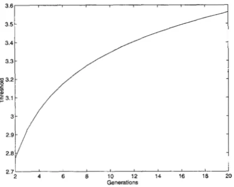
FIGURE 2.-Thresholds of test statistic X , at a significance level of 5% as a function of generation t.

hood ratio for testing Ho:a = 0 us. Hl:a f 0 for the

presence of a QTL at d and known

x,(&

is

[%I2.

When d is unknown, the log-likelihood ratio statistics becomes

max ___

d

{%i;r’

where the maximum is taken over all loci d where xt(

d)

is known. The variable x,(d) is known when a marker is available at d.

Now let

x,=&-.

G ( d )

d i g e

Along the same line as that of LANDER and BOTSTEIN (1989), we can show that, under the null hypothesis of Ho:a = 0, X , is a Gaussian process with mean 0 and covariance function R(u) = e-‘1u1 as n ”* m. Note that

for F2 data, R(u) = e-n1u1. This limiting distribution holds even when the e,‘s are not normally distributed (DUPUIS 1994). Therefore, X d i s still an Ornstein-Uhlen- beck process.

Using the results of FEINCOLD et aZ. (1993), we have Po(max X ,

>

b)

=

1 - @ ( b )

+

tZb+(b),

( 5 )

where

Z

is the length of the chromosome, +(x) and

@(x) are the density and cumulative functions of the

standard normal distribution, respectively. As an exam- ple, we calculated the threshold as a function of t for the test statistic X , at 5% level with 1 = 100 cM. The results are shown in Figure 2.

Thus, we can see that with a fixed significance level

a , increasing t will decrease 1 - @ ( b ) and hence in- (1

crease the threshold b. This can be explained intuitively. The recombination is a measure of genetic distance between the two linked loci. Increasing t corresponds effectively to increasing the number of recombination events, which in turn, is equivalent to increasing the genetic distances, or the length of the genome. This implies that we would search a QTL in a “longer” ge- nome. Therefore, to maintain the same significance level a of the test as in the F2 case, we need to increase the threshold of the test for F, data.

When the genetic map is not dense, ie., markers are not available at some locations, it is usually assumed that

x,(

d)

is known at equispaced distances of A cM. For the case where the xt(d) are only known at equispaced distance of

A

cM, (5) becomes

Po(max X ,

>

b)

=

1 - @ ( b )

+

tZb+(b)v(bJ2tA), (6)

where v( x)

=

e-o.583s (FEINGOLD et al. 1993). Note that this equation is equivalent to (5) when A = 0. Here, the function v ( x ) is a discreteness correction factor to account for the fact that we are computing the likelihood ratio statistic at discrete points on the chro- mosome instead of continuously as is the case for a dense map.

Similarly, when d is unknown, the log-likelihood ratio statistic for testing the dominant effect is

k

max Z:,

(7)

d

where

The threshold of the test is determined by

Po{max Zd

>

b]

=

1 - @ ( b )

+

2tZb+(b), ( 8 )

rl

if the genetic map is dense, or

Po{max

zk,

>

bl

=

1 - ~ ( b )

+

2tZb+(b)v(bJ4tA), (9)

if the map is equispaced map with the distances of

A

cM.

Next we address the issue of testing for the presence of either additive or dominance effect, which amounts to a general hypothesis H,: a = 6 = 0 us. Hl:a f 0 or

6 f 0. The corresponding log-likelihood ratio is

d

Thus, as n + 00,X , and Zd are Gaussian processes with

mean 0 and covariance function e - t 1 u 1 and e-2r1u‘, respec- tively. Moreover, X , and Z, are asymptotically indepen- dent (DUPUIS 1994).

i

I I

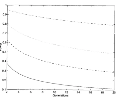
FIGURE 3.-Power of test with a significance level of 5%

and an additive effect a = 0.25 (0: is set to be 1). -, ---,

. . .

-

.

-

.

represent n = 100,200,300, and 500, respectively.

Po(max[X2(kA)

+

Z2(kA)] 2 t?]

=

e-'/" k

+

~ 6 ~ t b ( f i ) e - 1 ' ~ p 5 a. (10) The power of the test: The power of a test is the probability of detecting the effect of the QTL when it exists. To give an approximation to the power of the test, we need to calculate E [ X J under Hl:a f 0. Assume that there is a QTL, we can show in Appendix C that

E [ X d ]

=

(e"I"1, (11) where

5

= f i a / a , and

I

uI is the distance between the marker and the QTL.

Again, using the results of FEINGOLD et al. (1993), we obtain the following approximations:

(1) for a dense map

P,,(max X ,

>

6)

=

1 - @ ( b -

E )

d

+

+ ( b - 5)[2€" - ( b

+

' T l I , (12)

(2) for an equispaced map P,,,(max

>

b)

=

1 - @ ( b -

E )

k

+

+ ( b - <)[~E"v - ( b

+

<)"v'], (13)

where v =

~(6).

Although the formula for calculating the power of the test is the same in form for any F, population, the power of the test in F, population decreases with t be- cause increasing t means increasing the threshold as we have shown in the previous section.

Figure 3 shows the power of the test statistic X, for a significance level of 0.05 and an additive effect a = 0.25. Note that the power of the test in general decreases with increasing t, but the decreases in power for different sample sizes are different. The powers of the test for n

= 100, 200, 300, and 400 based on F,(, are 30%, 46%,

82%, and 98% as those based on F,, respectively. Thus, the reduction in power with increasing t is smaller for larger sample size.

Support intervals for QTL locations: The construc-

tion of a support interval for the QTL location on the chromosome is a useful way to assess the uncertainty in QTL localization. It also helps to narrow down the search of QTL to a small chromosomal region. Com- pared with that in F2 population, the length of support interval of mapping QTL in F, population will be dra- matically reduced.

To illustrate this, we use a lod-support interval. An a-lod support interval includes all the loci s such that

Zod( s) 2 max lod(

d)

- a , (14)

where lod(s) is the base-10 logarithm of the likelihood ratio statistic at the locus s.

From the previous section, we know that the asymp- totic log-likelihood ratio for testing H": a =

6

= 0 us.

Hl:a f 0 or 6 f 0 in the presence of a QTL at d is

ri

LR(d) =

X:

+

Z z . The lod score can be written as

lod(d) = '/2(log lOe)LR(d). (15)

Assuming there are k QTL, we know from the previ- ous section that, provided n is larger enough,

As we have shown in the previous section, the esti- mated genetic effects & (d) and

8(

d)

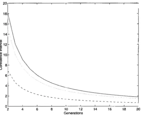
decrease exponen- tially with t as well as the distance between the marker and the QTL. As a result, the length of support interval of the QTL position will be reduced exponentially as t

increases. Figure 4 illustrates the expected length of the support interval using F, data. It can be seen that the expected lengths of the support interval decreases exponentially. The lengths of support interval using F, data are reduced by fivefold if Flo data are used. How- ever, there is a diminished return: only a further 1.8- fold reduction is achieved after another 10 generations. This agrees with what DARVASI and SOL.L.ER (1995) found in their simulations.

Kullback-Leibler (KL) distance and Fisher informa-

tion: To further characterize the gain in fine-scale mapping of QTL using the historical recombinations, we compute the KL distance between the probability distributions with true and estimated QTL locations. We also compute the Fisher information for the likeli- hood ratio.

Fine-Scale Mapping o f QTL 1207

20, I

"2 4 6 8 10 12 14 16 18 20

Generations

FIGURE 4.-Expected lengths of the support intervals of the estimated QTL locations using F, data. -, the case of n

= 100, LY = 0.5, 6 = 0.25; ---, the case of n = 1000, LY = 0.25, 6 = 0.1; * * e , the case of n = 500, LY = 0.25, 6 = 0.1. In all

cases, a: is set to be 1.

another when A is true (KULLBACK 1983a). Let y n be an estimated QTL map location and y* the true QTL map location. We can show (APPENDIX D ) that, for a dense map, the KL distance between the likelihood functions L ( y n ) and L ( y * ) , defined as K , ( L ( y * ) , L ( y n ) )

= E,*(log[L(r*)/L(r,)l), is given by

K(L(?.*) 3 U Y n )

1

where Or,,* is the frequency of the recombinant haplo- types between the locations y n and y*.

If 6 = 0, i.e., there is no dominant effect,

where 0, is the recombination fraction between y n and y * .

Thus, the KL distance K , ( L ( y * ) , L ( y , ) ) for F, data is approximately t/2 times greater than that for F2 data. In other words, the information for discriminating y* against y n is increased by t/2-fold.

KONG and WRIGHT (1994) showed that above result

implies that

as n ( y n - y*

I

+ co with the rate proportional to the

KL distance. Hence, with a large enough sample size and a dense map, the likelihood function will be con- centrated in intervals encompassing the true locations

QTL y * , with widths of the intervals in the order of 2/

nt in F, population, which is t/2 times narrower than that in F2 population. This further confirms that the widths of support intervals of the QTL location in F, population would be reduced by t/2 times.

If 6 f 0, we can show that (APPENDIX E )

-A:

U T ) d T

EIOeny*] = be (19)

where

1 2N(t) '

X ( t ) = 28,

+

-

Thus, K , ( L ( y * ) , L ( y , ) ) can be evaluated in principle by substituting E[B,,,*] = 1/2[1 - e?mf] and (19) into

(17).

Of course, the expression for K , ( L ( y * ) , L ( y n ) ) will become more complicated.

The generalized Fisher information of the likelihood ratio measures the amount of information supplied by the data about the unknown parameter, e.g., the QTL location y* (KULLBACK 1983b). However, the typical formula of Fisher information requires that the log- likelihood function be differentiable. Here, however, the log-likelihood ratio function is a function of the distance between y n and 7". Therefore, this log-likeli- hood ratio function is not differentiable at the true QTL map location y*. Thus, the formula for calculating the Fisher information cannot simply be applied to our case. KONC (A. KONG, personal communication) modi- fied the formula of Fisher information to allow a nondif- ferentiable log-likelihood function at the true parame- ter as follows.

Suppose that a random variable X is distributed with density

p(

x,

e)

and 6 is an estimator of g(6). Further- more, assume that

Here, we can show that (APPENDIX F ) , in our case,

The Fisher information Z(e) is defined as

FIGURE 5.-The Fisher information as a function of popula- tion size. -, ---, * * ,

-

* - * are Fisher informations for n =

100, 500, 1000 and 10000, respectively.

ing the difficulty of estimating the true QTL location

y* in

fi

population as

For the ease of exposition, we use the first-order of approximate to the likelihood ratio. In APPENDIX G, we show that

U Y " )

=

-

( a - 6)' [2(26 - a ) 4

+

2(26

+

a ) 4

8a4

+

46(26 - a)'(2S

+

a )

+

2(46' - a2)']

+

b(a - b)a'

2a4 [(26 - a)'

+

3(26

+

a)*]

@a4 ( a - b)2

2a4

2a2

+-+-

(86'

+

5a2 - 8a6)

+

b ( a - 6)

a2 a ( a

+

2 4 ,

where

t a = - -

2 '

If we assume N ( t ) =

N,

then b = - (?/16N). To see how the Fisher information increases as generation t increases, we calculated the Fisher information for a =

6

= 0.5, and a* = 1 (Figure 5 ) . We can see that the Fisher information increases as the generation t in- creases, which implies that the observed data sampled from an F, population contain more information about the true QTL location than that in F2 population. It

also can be seen from the figure that, for t 5 12, the

Fisher information for data sampled from populations with different sizes (100, 500, 1000, and 10000) are practically identical. After 12 generations, the Fisher information for data sampled from populations of >500 are indistinguishable. However, the difference in Fisher information increases as t increases for N = 100 and N = 500. These observations suggest that for t 5

12, an effective population size of 100 should be enough. This seems to agree with DARVASI and SOLLER

(1995). For t

>

12, however, a population size of > l o 0 is recommended. This is because that, while a popula- tion of 100 individuals may be large enough to avoid genetic fixation for t 5 12, it may not be large enough

if further intercrossing is required.

EXTENSION TO THE MULTIPLE

REGRESSION MODEL

The previous analysis can be extended to the multiple regression model for fine-scale mapping of QTL using F, data. Assume n individuals are sampled at random from an F, population. For the zth individual ( i = 1,

. . .

,

n), denote the corresponding quantitative trait value as

x,

and marker genotype (codominant) at jth locus as

Mi(

I ] ( j = 1,

. . .

,

m). Assuming no epistasis and no interaction between environment and QTL, the multi- ple regression can be written as follows:

1

+a, - 6, M , ( j = AA

Y , = p + c

6, Mt( J ) = AB

+

t, for an F,, (22)

,=

1

-a, - b] Mt(J = BB

where a] and 6, are additive and dominant effects associ- ated with thejth marker, et's are independent and iden- tically distributed random variables with E[€,] = 0 and Var(e,) = 2 .

Let X , be a row vector containing the coefficient of the parameters p, a and

6

in

(22)

and X = [X:;

. . .

,

X;]? In matrix notations, (22) can be rewritten as

Y =

+

E, E[&] = 0 , V(E) = a21, (23)

where

p

= [ p , a , ,

. . .

,

am, SI,

. . .

,

dm]. It is a classical result that the least square estimate of

0:

/j = ( X T X ) " X T y .

By the strong law of large numbers (RODOLPHE and LEFORT 1993),

-

xrx

= - XFX, + E[X:jr,] =

u,

1 , 1 " d . S

n 2 = 1

Fine-Scale Mapping of QTL 1209

...

...

...

...

1 0 0 0 0 0

0 A1 0 0 0 0

0 0 A2 0 0 0 0

0 0 0

...

A, 0 0

...

0 0 0

...

0 B1 0

...

0 0 0 0

...

0 0

&

...

0 0 0

...

0 0 0

...

...

...

. . .

...

where A, and B, denote the matrices of additive and dominance effects in the zth chromosome respectively. We can show (APPENDIX H ) that for F, data

A, = [&-fA1l,] and B, = [e-'"a,,<],

where A,,' is the genetic distance between the markers j and

j ' .

It can be seen that the matrix U, for the F, data has the same structure as that for the F2 data. If all genetic distances A,j8 increase by t / 2 fold, the matrix U, for the F2 data become identical to U,.

Since

a. 5

n Var(0) = n

o2(xT4-'

--t Q'U"

by the Central Limit Theorem, we have

& ( f i n

-

0)

-

N ( 0 , a'u-l).

Hence, , b n is a n unbiased and consistent estimator

Asymptotic variance of the estimated genetic ef-

fects:

As

we mentioned before, the matrix U, has the same structure of the matrix Uin F, population. There- fore, using similar arguments as that of RODOLPHE and LEFORT (1993), we have

of

p.

2 t = - V(&J

and

2 t

= - V(

6J

,

where V(&J and V(6,) are the variances of & j and

8,,

estimated by multiple regression using F2 data (Ro? DOLPHE and LEFORT 1993). It can be seen from the

above equation that, as the distance between adjacent

markers get smaller, i e . , the marker density increases, both V(&J and V(6]) increase, which makes it difficult to increase the resolution of mapping QTL.

We can see from above that one way to effectively use dense map and retain small variances of estimated genetic effects is to map QTL by F, data. Indeed, the variances of the estimated additive and dominance ef- fects by multiple regression for F, data are reduced ap- proximately by t / 2 times as compared with F2 data. Thus, the use of F, data will be more effective in separat- ing individual QTL when they are linked, and provide greater precision of the estimated genetic effects.

Note that for the simple regression, since

u,=

0 %I 0

...

0 0 0

...

0 0 0

gz

* * * 0 0 0 * * - 0

0 0 0

...

%I 0 0

...

0

i

1 0 0 * * . 0 0 0

.*.

0

...

_{0 0} * * * 0

0 0 0

...

0 I 0

...

0 0 0 0

...

0 0

z

...

0

0 0 0

...

0 0 0

...

I

...

we have

V ( s i ( t ) ) = V(&j) and V ( d , ( t ) ) = V(6,).

This suggests that for the simple regression model, increasing t has no effect on variances of the estimated genetic effects.

Effects of

QTL:

By the same argument as that of

RODOLPHE and LEFORT (1993), we can show that using F, data to map QTL does not destroy the most important property of multiple regression model for mapping QTL: the genetic effects associated with the markers depends on only those QTL that are located on the interval flanked by the two neighboring markers, and is independent of the effects of QTL located on other intervals. Therefore, to calculate the effects of QTL as- sociated with the marker, we need to consider only those QTL located in the interval flanked by neigh- boring markers.

The increase of recombination events, as a result of the use of historical recombinations, effectively in- creases genetic distances between the markers and QTL. Therefore, as in the case of the simple regression, the estimated additive and dominance effects due to QTL will be reduced quickly when moving away from QTL. In this subsection, we evaluate the amount of the reduction as a function of t.

Using the same argument as that of RODOLPHE and LEFORT (1993), we can show that (APPENDIX I )

where K is the number of QTL located between marker

j - 1 and marker j , bk and ck are additive and dominance

effects of the kth QTL, respectively.

To quantify how much the additive and dominance effects, associated with the markers, in Ff population are reduced, we assume, for simplicity, that only a single QTL is located between markers j - 1 and j . This as- sumption holds when the genetic map is dense enough. Then, after some algebra, we have

and

where Ai, is the genetic distance between the marker j and the QTL and a j ( 2 ) and 6,(2) are the additive and dominance effects estimated from F2 data. Thus, the estimated genetic effects decrease exponentially as one moves away from QTL, with the dominant effect de- creasing faster than the additive effect.

Recall that

-

N ( p , a2U"), and that variances of the additive and dominance effects based on F, data decrease linearly with t as compared with those based on F2 data. Taken together, it is easy to visualize that

ej(t)

and Aj(t) will be concentrated on the increasingly narrow region surrounding the QTL. Consequently, the "ghost locus" and other problems associated with using F2 data in mapping QTL will be alleviated significantly using F, data.

Support intervals for QTL locations: Suppose that we have estimated the location of QTL, which is flanked by the markers M, and Mc+l. Now we want to consider the confidence interval for the estimated location of QTL

q.

From classical regression theory (GFWBIL 1976),

it is well-known that the likelihood ratio statistic for testing Ho:a =

S

= 0 us. H l : a # 0 or

6

# 0 is given by

LR = Y r ( x x - - &X,-) Y

a'

where XX- = X ( X ' x ) - ' X T and

X,

= [ 1 1 *

-

11':

The lod score can be written as

lod =

&

log,, eLR

which can be approximated asymptotically by

L_I= . _{I I = 1}

where a] and Sj are the statistic additive and dominance effects at the marker j defined in the previous section. If A j k is the genetic distance between the marker Mj

and the kth QTL in the interval flanked by the markers

M, and and bk and ck are the corresponding addi-

tive and dominance effects of the kth QTL, respectively,

k= I

k= 1

where 4 is the number of QTL in the jth interval. For simplicity, suppose that we have a dense map and the marker M,, located at locus d in the i interval [Mi, M 2 + 1 ] , is used to detect the location of QTL. Adding this marker to the set of the original markers, and re- gressing the phenotypic value Yon this augmented set of the markers yields an approximation to the asymp- totic likelihood ratio statistic:

LR(d) = - n

+

+

a,

2

where

kd

k= 1

k= 1

n m

n

a = 0

C

upl

+ n

u,6,,

,=I I = 1

and kd is the number of QTL in the interval flanked by the markers [ M t , M d ]

.

Recall that an x-lod support interval is an interval including all the loci s such that

lod(s) 2 max lod(

d)

- x. ( 2 6 )

To determine the support interval, we need to calcu- late maxd lod(d). For simplicity, assuming that there is only a single QTL, indexed as

q,

in that interval. Then,

d

Substitute this into ( 2 6 ) , and find a marker located at

d, such that

where Adt4 denotes the genetic distance between the marker located at dl and the QTL q or half a-lod support interval in F, population, denotes the

Fine-Scale Mapping of QTL 1211

and

To see how much the length of the support interval for a QTL map location is reduced by multiple regres- sion model using F, data, we assume cq = 0, i.e., there is no dominant effect. After some algebra, we have

e-2A +4tAd = @

9 P

,

63

where Adtq and A&, are half of the length of the a-lod support interval for a QTL map location by multiple regression using F, and F2 data, respectively. It is easy to see that, for t

>

2,

- gz

>

1.

gt

Hence,

That is

which means that the length of an a-lod support inter- val for a QTL map location by multiple regression using F, data will be reduced by more than t/2 fold.

Threshold and power: For a particular chromosomal interval flanked by two markers, the statistic genetic effects estimated through the multiple regression de- pend only on those QTL located within the interval. It is thus natural to test whether or not there exists a QTL in a given interval. Suppose that we want to test the interval [Mj-,, M j ] . Similar to the simple regression model, we let

and

where

&(d)

and

6(d)

are associated with a marker lo- cated at locus d in the interval [MI-,, Mj] and are esti- mated by the multiple regression method.

It can be shown that under the null hypothesis of

Ho:bq = 0 and cq = 0, X , and Z, are asymptotically Gaussian processes with mean 0 and a complicated co- variance function, which can be approximated by the

function R( u) = e - f 1 u 1 . Therefore, x d and z d can be

approximated by an Ornstein-Uhlenbeck process. To determine the thresholds of the test, we can use formulae similar to

(5),

( 6 ) , (8), (9), and

( l o ) ,

but with the length of genome replaced by the length of the interval. Consequently, for fixed t, the threshold of the test becomes lower.

Assume that in the interval [Mj-,, M,] there exists only one QTL with additive and dominance effects bk

and ck, respectively. Under H,:bk f 0 or ck f 0, we have

The coefficient of e-"dk depends in general on the

genetic distance between the marker and the QTL and do not have the form of (1 1). However, if Adk is small,

E [ &

(d)

] can be approximated by

E [ & ( d ) ] bke-lA,k.

In this case, letting ( = d E ( b k / a , ) , (12) and (13) can still be used for calculating the power. Note that

[ is independent of the time and the length of the interval.

As

we discussed before, increasing the number of recombinant events is effectively equivalent to increas- ing the genetic distance between loci, and hence to decreasing the genetic effects of QTL. Therefore, to maintain a prespecified type I error, we need to increase the threshold of the test, which, in turn, will decrease the power of detecting QTL. To increase the power of detecting QTL in the particular interval, we can reduce the length of the interval. If the product t l i s kept con- stant, then we know from (5) that the threshold of the test will remain constant, as will the power.

DISCUSSION

With increasing popularity of QTL mapping in eco- nomically important animals and in experimental spe- cies, the need for statistical methodology for fine-scale QTL mapping becomes increasingly urgent. An obvious approach is to increase sample size to increase the re- combination events. However, this approach is often constrained by resources. Moreover, as shown by HYNE

et al. (1995), increasing the sample size beyond a certain point will not further reduce the length of confidence interval for QTL map locations.

Xiong and S.-W. Guo

fects, the multiple regression model does. To further understand the advantages and disadvantages of using F, data relative to F2 data, we have calculated the Kull- back-Leibler distance and Fisher information for the simple regression model. In addition, to help imple- ment fine-mapping methods, we have derived the for- mula to compute the power and threshold values for both the simple and multiple regression models.

The idea behind the work of DAVASI and SOLLER (1995) is to use historical recombinations for fine-scale mapping. This idea has been known in human genetics for about 10 years, although it has recently been shown to be quite successful in locating disease genes in fine scale (HASTBACKA et al. 1994). The idea is simple in- deed: in the absence of selection, the linkage disequilib- rium between any QTL and marker loci, however closely linked they are, will gradually dissipate as the population continues intercrossing. Hence, the evolu- tion of haplotype frequencies in the population reflects the action of recombination through past generations, making it possible to disentangle and finely map closely linked QTL.

It should be pointed out that, although the popula- tion model that we considered is for the F, population, or, in DAVASI and SOLLER’S terms, the AIL design, the model and subsequent analysis can be modified easily to allow for other features such as selection or particular design.

The analytical techniques that we used in this paper enable us to discover much more interesting features of fine-scale mapping via historical recombinations than found by simulation studies. We have demonstrated that, since the estimated additive and dominance effects based on F, data decrease exponentially as one moves away from QTL, the length of the support interval for the estimated QTL map location also decreases expo- nentially with t and by approximately t / 2 fold. We also have demonstrated that, for the simple regression model that was investigated by DAVASI and SOLLER (1995), the variance of estimated genetic effects using F, data is the same as that in F2 population. In other words, there is no gain in precision in estimation of the genetic effects using the simple regression even F, data are used. If, however, a multiple regression model is used, that variance will be reduced approximately by t / 2 times as compared with F2 data.

By extending the definition of the Fisher information to the case of nondifferentiable likelihood functions, we have showed that, for the simple regression model, the Fisher information evaluated at the true QTL loca- tion with F, data is much larger than that for F2 data. We also have used Kullback-Leibler distance to measure the rate of convergence of the estimated QTL map location to the true QTL location. We found that that Kullback-Leibler distance between the likelihood func- tion evaluated at estimated QTL map location and at the true QTL location using F, data is approximately

t/2 times as large as that using F2 data. Thus, for the simple regression model, the information on QTL loca- tions using F, data is much higher than that for F2 data.

To help implement fine-scale mapping of QTL using F, data, we have evaluated the thresholds of the test for both simple and multiple regression models. Intuitively, increasing t means more accumulated recombinant events, which is effectively equivalent to increasing the genetic distances, or the length of the genome on which QTL are being searched. Consequently, the thresholds of the test for F, data should be higher. We have showed that the thresholds for the test of QTL for a genome segment of length

I

with F, data are roughly equal to those for a genome segment of length tl with F2 data.

As a result, the power of detecting QTL for a giuen

marker will be reduced. This seems to contradict with the common perception that experimental parameter values that increase/decrease the power also tend to decrease/increase the lengths of support (or confi- dence) intervals for QTL map locations. This apparent contradiction can be easily resolved by noting that here the power refers to the power of the test for whether or not there exists a QTL for a given marker, not the power of testing the QTL locations. In addition, be- cause the genetic effects decrease exponentially as one moves away from the QTL, the length of support inter- val for QTL location also decreases exponentially, thus increasing the precision of estimation of QTL map loca- tion. This point has been made by DAVASI and SOLLER

(1995) using a simple argument. Based on our analysis, the point can be illuminated more clearly.

We point out, however, that the use of historical re- combinations in fine-mapping QTLs is not without limit. In fact, as shown in Figure 4, there is a diminished return with increasing tin terms of increasing the preci- sion of the estimation of QTL map location. The great- est gain in precision seems to be achieved in the first eight to 10 generations after FB. This suggests that for

t 2 10, the use of F, data may not be very cost-efficient.

Since increasing the mapping resolution by using his- torical recombinations will result in decrease in power of detecting QTL, one might want to use a denser ge- netic map to detect QTL. However, increasing the den- sity of the map will increase the variances of the esti- mated genetic effects at the markers, which will cause difficulty in increasing mapping resolution. To main- tain the power of detecting QTL while improving the accuracy of estimated QTL map location, it may be appropriate to use a two-stage mapping strategy. First, use a sample of moderate size taken from the F:! popula- tion and a map with moderate density to detect QTL. Second, once the existence of QTL in some regions is detected, one can proceeding by fine-scale mapping using F, data.

Fine-Scale Mapping of QTL 1213

crossing and for which inbred lines exist. As DARVASI and SOLLER (1995) pointed out, inbred lines of mice, chicken, corn and cultivars as well as accession lines of most annual selfing plant species are good candidates for F, population. Furthermore, the time scale required for production of a F, population applies only to the first time that such a population is produced. In plant species, an F,, once produced, can be stored in the form of seeds, and constitute a permanent mapping population. In mice, or other animals, once an Flo, say, has been produced, it can be maintained by reproduc- ing at a much slower rate. Hence, for a relative small investment, such produced population can be used as resource population for fine mapping.

This research was supported by the National Institutes of Health grants R29-GM-52205 and ROl-GM-56515.

LITERATURE CITED

BODMER, W. F., 1986 Human genetics: the molecular challenge. Cold Spring Harbor Symp. Quant. Biol. Lk 1-13.

CHURCHIIL., G. A., J. J. GIOVANNONI and S . D. TANKSLEIY, 1993 Pooled-sampling makes high-resolution mapping practical with DNA markers. Proc. Natl. Acad. Sci. USA 90: 16-20.

DARVASI, A,, and M. SOLLER, 1995 Advanced intercross lines, an experimental population for fine genetic mapping. Genetics 141: 1199-1207.

DARVASI, A., V. WEINREB, J. MINKE, I. WELLER and M. SOLLER, 1993 Detecting marker-QTL linkage and estimating QTL gene effect and map location using a saturated genetic map. Genetics 134:

DAVIES, J. L., Y. KAWAGUCHI, S. T. BENNETT, J. B. COPEMAN, H. J. COR- DELL et al., 1994 A genome-wide search for human type 1 diabe- tes susceptibility genes. Nature 371: 130-136.

DIETRICH, W. F., J. MILLER, R. STEEN, M. A. MERCHANT, D. DAMRON- BOLES et al., 1996 A comprehensive genetic map of the mouse genome. Nature 380: 149-152.

DUPUIS, J. 1994 Statistical problems associated with mapping com- plex and quantitative traits from genomic mismatch scanning data. Technical Report No. 2. Department of Statistics, Stanford University, Stanford, CA.

ETHIER, S., and T. G. KURTZ, 1986 Markov Processes: Characterization and Convergence. Wiley, New York.

FEINGOLD, E., 0. P. BROWN and D. SIECMUND, 1993 Guassian mod- els for genetic linkage analysis using complete high-resolution maps of identity by descent. Am. J. Hum. Genet. 53: 234-251. GRA~II-I,, F. A,, 1976 Themy and Application of the Linear Model.

Wordsworth & Books/Cole Advanced Books & Software, Pacific Grove, CA.

WEY, C. S . , and S . A. KNorr, 1992 A simple regression method for mapping quantitative trait loci in line crosses using flanking markers. Heredity 69: 315-324.

W E Y , C. S., S. A. KNOTT and J. M. ELSEN, 1994 Mapping quantita- tive trait loci in crosses between outbred lines using least squares. Genetics 136: 1195-1207.

HASHIMOTO, L., C. HABITA, J. P. BERESSI., M. DELEPINE, C. BESSE et al., 1994 Genetic mapping of a susceptibility locus for insulin- dependent diabetes mellitus on chromosome llq. Nature 371:

WTBACKA, J., A. DE IA CHAPELLE, M. M. MAHTANI, G. CLINES, M. P. REEVE-DALY et al., 1994 The diastrophic dysplasia gene encodes a novel sulfate transporter: positional cloining by fine-structure linkage disequilibrium mapping. Cell 78: 1078-1087.

HYNE, V., M. J. KEARSEY, D. J. PIKE and J. W. SNAPE, 1995 QTL analy- sis-unrealiability and bias in estimation procedures. Mol. Breed. 1: 273-282.

JANSEN, R. C., 1989 Estimation of recombination parameters be- tween a quantitative trait locus (QTL) and two marker loci. Theor. Appl. Genet. 78: 613-618.

943-951.

161-164.

JANSEN, R. C., 1993 Interval mapping of multiple quantitative traits. Genetics 136: 205-214.

JENNINGS, H. S., 1917 The numerical results of diverse systems of breedingh special relation to the effects of linkage. Genetics 2: 97-154.

KARLIN, S., and H. M. TAYLOR, 1981 A Second Coursr in Stochastir Processes. Academic Press, Inc. New York.

KNAPP, S . J., W. C. BRIDGES and D. BIRKES, 1990 Mapping quantita- tive trait loci using molecular marker linkage map. Theor. Appl. Genet. 79: 583-592.

KNOTT, S . A,, and C. S . HALEY, 1992 Maximum likelihood mapping of quantitative trait loci using full-sib families. Genetics 132: 1211-1222.

KONG, A,, and F. WRIGHT, 1994 Asymptotic theory for gene m a p ping. Proc. Natl. Acad. Sci. USA. 91: 9705-9709.

KULLBACK, S., 1983a Fisher information, pp. 115-118 in Encyclopedia

of Statistics, Vol. 3, edited by S. KOTZ and N. L. JOHNSON. John Wiley, New York.

KULLRACK, S., 1983b Kullback information, pp. 421-425 In Encyclo- pedia of Statistics, Vol. 4, edited by S . KOTZ and N. L. JOHNSON. John Wiley, New York.

LANDER, E. S . , and D. BOTSTEIN, 1989 Mapping Mendelian factors underlying quantitative traits using RFLP linkage maps. Genetics 121: 185-199.

LANGE, R , L. KUNKEI., J. ALDRIDGE and S . A. LATT, 1985 Accurate and superaccurate gene mapping. Am. J. Hum. Genet. 37: 853- 867.

LEWONTIN, R. C., and K. KOJIMA, 1960 The evolutionary dynamics of complex polymorphisms. Evolution 1 4 450-472.

MARTINEZ, O., and R. N. CURNOW, 1992 Estimating the locations and the sizes of the effects of quantitative trait loci using flanking markers. Theor. Appl. Genet. 85: 480-488.

PATERSON, A. H., J. W. DEVERNA, B. LANINI and S. D. TANKSLEY, 1990 Fine mapping of quantitative trait loci using selected overlapping recombinant chromosomes in an interspecies cross of tomato. Genetics 124: 735-742.

RISCH, N., S. GHOSH and J. A. TODD, 1993 Statistical evaluation of multiple-locus linkage data in experimental species and its rele- vance to human studies: application to nonobese diabetic (NOD) mouse and human insulindependent diabetes mellitus (IDDM).

Am. J. Hum. Genet. 53: 702-714.

ROBRINS, R. B., 1918 Some applications of mathematics to breeding problems. 111. Genetics 3: 375-389.

RODOLPHE, F., and M. LEFORT, 1993 A multi-marker model for de- tecting chromosomal segments displaying QTL activity. Genetics

TANKSIXY, S . D., 1993 Mapping polygenes. Annu. Rev. Genet. 27:

THODAY, J. M., 1961 Location of polygenes. Nature 191: 368-370. TODD, J. A., C. MIJOVIC, J. FLETCHER, D. JENKINS, A. R. BRADW,LL et al.,

1989 Identification of susceptibility loci for insdindependent diabetes mellitus by trans-racial gene mapping. Nature 338: 587- 589.

WELIER, J. I., 1986 Maximum likelihood techniques for the map- ping and analysis of quantitative trait loci with the aid of genetic markers. Biometrics 42: 627-640.

WRIGHT, F., 1994 Asymptotics and Robustness f w Genetic Linkage M a p ping. Ph.D. thesis, University of Chicago.

ZENG, Z. B., 1993 Theoretical basis for separation of multiple linked gene effects in mapping quantitative trait loci. Proc. Natl. Acad. Sci. USA 90: 10972-10976.

ZENG, Z. B., 1994 Precision mapping ofquantitative trait loci. Genet- ics 136: 1457-1468.

134: 1277-1288.

205-233.

Communicating editor: W. J. EWENS

APPENDIX A

Assume that the recombination between loci 1 and

where

6,=

{

1 i f i = j

0 otherwise.

In particular, applying ( 2 8 ) for P& and P& ( t) yields

P & ( t ) = %&(t - 1 )

+

% P d t - 1 )

+

%Pll(t - 1)PH

x

( t - 1)

+

%R2*(t - 1)Pl2(t - 1 )

8

2

x

P22(t- 1)

+

- P11(t- 1)P22(t- 1)

Since we are mainly concerned with recombinant hap- lotypes r, = P12 ( t )

+

Pz1 ( t ) , we obtain, by summarizing

( 2 8 ) and (29),

ry = P & ( t )

+

P*21(t) = ?--I

+

2 8 [ P , , ( t - 1 )

X P22(t - 1 ) - P12(t - 1)P21(t - I ) ] . ( 3 0 )

Since the population F, are produced by randomly mat- ing from an F2 population, the expectation of frequen- cies PI ( t ) and P2* ( t ) will be identical. The same is true for P12(t) and ( t ) . Thus,

PIl(t - 1 ) = Pz*(t - 1 ) = % ( 1 - 7 - , - 1 ) ,

PI*( t - 1 ) = P21(t - 1 ) = X q - 1 . ( 3 1 )

It follows from ( 3 0 ) and ( 3 1 ) that

0

7-*

- -

+

(1 - O)rt-l

- 2 ( 3 2 )

or

Thus, the population process { X ( t) = number of recom- bination haplotypes at the tth generation} evolves as a Markov chain with the transition probability

which can be approximated by the diffusion process with a generator given by (KARLIN and TAYLOR 1981)

L = r,( 1 - 7-J

8

2 N ( t )

a??

-

+

(:

- - ort

)

- .

R",

( 3 3 ) APPENDIX B

Suppose that there are K QTL with the kth QTL, located at dk, having additive effect ( Y k and dominance

effect 6,. Then, the true model is

K K

yi = /I.

+

(Y&( dk)

+

6kZE( dk)

+

e,, 2 = 1 , 2,

. .

.

,

n,

k= 1 k= 1

where x j ( d k ) and z i ( d k ) are indicator variables with the values

and

where Q and q are two alleles of the QTL. Recall that in the text we assumed the following simple linear re- gression model:

yz = p

+

a x ,

+

Sz,

+

ei, i = 1, 2 ,

. . .

, n, ( 3 4 ) where x, and

zi

are dummy variables representing the genotype at the marker M,.

It is easy to see that

E[x1 - F 1 2 = ( 1 - ; ) E [ $ , = ( 1 -

;)

By the strong law of large numbers, we obtain 1 "

-

2

[x, -

$1'

"t l / 2 . a. r , = I

( 3 5 )

Now we calculate E [ x i ( dk) x i ) ] . Let P k ( t ) be the expecta-

tion of the recombinant haplotype at the marker M and the k h QTL. It can be shown that

Fine-Scale Mapping of QTL 1215

and

we have

Let

q n . n

Then,

Thus,

Therefore, combining (35) and (36) yields

1

n n. c

1 n

- Z I [yt - $xt K

& ( t ) =

x

ffke-"k.

-x:=,

[ x i - $ 2 k=I

Similarly, by noting that

E[zi( dk) &'] = %e-2ak,

E[xi(dk)zil = 0 ,

k= 1

APPENDIX C

Suppose a QTL is located at s. Then, from standard regression analysis, we have

Recall that in APPENDIX B, we showed that

Clearly,

By the strong law of large numbers, we have

APPENDIX D

Assume that the map is dense. Given observed pheno- types y = [yl,

.

. .

, yn] Tand the genotypes of the markers M ( y * ) = [Ml ( y * ) ,

. . .

, M,( y * )

3

'

under the true QTL map location y* as well as M ( y n ) = [MI ( y n ) ,

. . .

,

M n ( y n ) l T under an alternative yn, the log likelihood ratio log(L(y, y*)/L(y, yn)) can be expressed as

where

and y is the assumed QTL map location. After some calculations, we have