SERIES REPRESENTATION OF POWER FUNCTION

SERIES REPRESENTATION OF POWER FUNCTION

KOLOSOV PETRO

Abstract. In this paper we discuss a problem of generalization of binomial distributed triangle,

that is sequence A287326 in OEIS. The main property of A287326 that it returns a perfect cube

n as sum of n-th row terms over k, such that 0 ≤ k ≤ n−1 or 1 ≤ k ≤ n, by means of its symmetry. In this paper we have derived a similar triangles in order to receive powersm= 5,7 as row items sum and generalized obtained results in order to receive every odd-powered monomial

n2m+1, m≥0 as sum of row terms of corresponding triangle. In other words, in this manuscript are found and discussed the polynomialsDm(n, k) andUm(n, k), such that, when being summed up overk in some range with respect tomandnreturns the monomialn2m+1_.

Contents

1. Structure of the manuscript 1

2. Introduction 2

3. Generalization of sequence A287326 6

3.1. Properties ofDm(n, k) and Am,j 12

3.2. Example of use of theorem (3.30) 13

4. Another power identity 15

5. Acknowledgements 22

6. Conclusion 23

References 23

7. Application 1. Extended tables of polynomials, consistingUm(n, k) coefficients 24

1. Structure of the manuscript

The problem of finding expansions of monomials, binomials, trinomials, etc. is classical and a lot of theorems have been found, the most prominent examples are Binomial Theorem [2], Multinomial theorem, Worpitzky Identity [30], [34], Stirling numbers of second kind and falling factorial identity, [36], etc. In this paper we try to solve the classical problem of finding expansions of monomials. We start from binomial distributed triangle A287326, [11] in OEIS. The main property of A287326 that it returns a perfect cubenasn-th row sum, starting from 0, ..., n−1 or from 1, ..., nby means of its symmetry. Therefore, the following question stated:

• Is there a generalization of A287326 in order to receive monomial nt, t >3 as sum of n-th row terms of corresponding triangle, where t is natural?

Finding an analogs for t = 5,7 in section 3, we answer to above questions positively. Could this process be continued for each oddt= 1,3,5,7...similarly? Positive answer to this question is given by theorem (3.30).

Date: August 17, 2018.

Key words and phrases. Series Representation, Power function, monomial, Binomial Theorem, Multinomial the-orem, Worpitzky Identity, Stirling numbers of second kind, Faulhabers sum, finite difference, Faulhabers formula, central factorial numbers, binomial coefficients, Binomial distribution, binomial transform, Bernoulli numbers, OEIS, multinomial coefficients.

1

2. Introduction

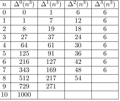
Let describe the derivation of the sequence A287326 in OEIS. Sequence A287326 returns the perfect cube nas row sum over k, 0≤k≤n−1, as well as sum over 1≤k≤n, by means of its symmetry. First, consider a difference table of perfect cubes ([4], eq. 7)

(2.1)

n ∆0(n3) ∆1(n3) ∆2(n3) ∆3(n3)

0 0 1 6 6

1 1 7 12 6

2 8 19 18 6

3 27 37 24 6

4 64 61 30 6

5 125 91 36 6

6 216 127 42 6

7 343 169 48 6

8 512 217 54 9 729 271

10 1000

Table 1: Difference table of perfect cubesn, 0≤n≤10 up to 3rd _order. Reviewing above table, we have noticed that

∆(03) = 1 + 6·0 = 6 1₂+ 1₀ (2.2)

∆(13) = 1 + 6·0 + 6·1 = 6 2₂+ 2₀

∆(23) = 1 + 6·0 + 6·1 + 6·2 = 6 3₂+ 3₀

∆(33) = 1 + 6·0 + 6·1 + 6·2 + 6·3 = 6 4₂+ 4₀ ..

.

∆(n3) = 1 + 6·0 + 6·1 + 6·2 +· · ·+ 6·n= 6 n+1₂ + n+1₀

Above difference identity is closely related to Faulhaber’s sum of cubes, wheren3= 6 n+1₃ + n+1₁ , see ([21], p. 9). Note that ∆2(n3) could be found similarly using above identity, i.e ∆2(n3) = 6 n+1₃₋₂

+ n+1₁₋₂

.

Property 2.3. (Generalized finite difference of power using Faulhaber’s formula). Consider the identities, ([21], p. 9). For every odd power



       

       

n1 = n₁

n3 = 6 n+1₃

+ n₁

n5 _{= 120} n+2 5

+ 30 n+1₃

+ n₁

.. . n2m−1 = P

1≤k≤m

(2k−1)!T(2m,2k) n+k_2k−−₁1

The coefficients in these formulas are related to what Riordan[22] has called central factorial num-bers of the second kind. In his notation,

xm = X

1≤k≤m

T(m, k)x[k], x[k]=x(x+k₂ −1)(x+k₂ −2)· · ·(x+k₂ + 1)

The coefficients T(2m,2k) are always integers, because the x[k+2] =x[k](x2/k4) implies the recur-rence

We can find the first order finite difference of odd power as decreasing the variable of corresponding binomial coefficients by 1, for example



       

       

∆n1 = n₀ ∆n3 = 6 n+1₂

+ n₀

∆n5 _{= 120} n+2 4

+ 30 n+1₂

+ n₀

.. .

∆n2m−1 ₌ P

1≤k≤m

(2k−1)!T(2m,2k) n+k_2k−−₂1

Continue similarly, we can express each difference of order t ≥1. The central factorial numbers of the second kind (2k−1)!T(2m,2k) in above identities are terms of OEIS sequence A303675 and generated by

(2.4) (2k−1)!T(2m,2k) = 1

r

r

X

j=0 (−1)j

2r j

(r−j)2n=:Vm,k,

where r=n−k+ 1, this formula was provided by Peter Luschny in[27]. Repeated sums are equally easy, in Knuth’s notation (see [21], p. 10)

Σrn2m+1 = X 1≤k≤m

Vm,k

n+k+r

2k−1 +r

Therefore, reviewing the difference as inverse operator to summation for every oddt >0andm≥0, we have identity

∆rn2m+1 = X 1≤k≤m

Vm,k

n+k−r

2k−1−r

By property 2.3 we rewrite the cubes as

(2.5) n3 = X

1≤k≤n 6

k+ 1 2

+

k

0

Rewrite above expression with set every binomial coefficient to be n+1₂

= 1 + 2 +· · ·+ (n+ 1), then

n3 = (1 + 6·0) + (1 + 6·0 + 6·1) +· · ·+ (1 + 6·0 +· · ·+ 6·(n−1)) Particularizing above expression, we get

(2.6) n3 =n+ (n−0)·6·0 + (n−1)·6·1 +· · ·+ (n−(n−1))·6·(n−1)

Provided that nis natural. Now, let apply a compact sigma notation on (2.6), thus

(2.7) n3 =n+ X

1≤k≤n

6k(n−k)

As sum P

1≤k≤n6k(n−k) consists of n terms, we have right to move n in (2.7) under sigma notation, we get

(2.8) n3 = X

1≤k≤n

6k(n−k) + 1

Property 2.9. (Proof of symmetry). Let be a setsA(n) :={1, 2, . . . , n}, B(n) :={0, 1, . . . , n}, C(n) :={0, 1, . . . , n−1}, let be expression (2.8) denoted as

M(n, C(n)) = X k∈C(n)

where n is natural-valued variable and C(n) is iteration set of (2.8), then we have equality

(2.10) M(n, A(n)) =M(n, C(n))

Let review and denote expression (2.6) as

U(n, C(n)) = n+ 6· X

k∈C(n)

k(n−k)

then

(2.11) U(n, A(n)) =U(n, B(n)) =U(n, C(n))

Other words, changing of iteration sets of(2.6) and (2.8) by A(n), B(n), C(n) and A(n), C(n), respectively, doesn’t change resulting value for each natural x.

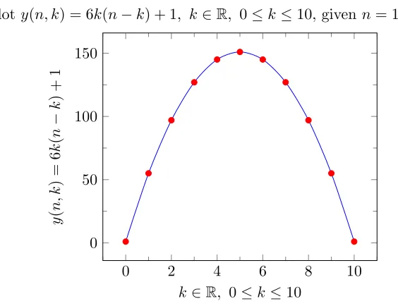
Proof. Let be a ploty(n, k) = 6k(n−k) + 1, k∈_R, 0≤k≤10, givenn= 10

0 2 4 6 8 10

0 50 100 150

k∈R, 0≤k≤10

y

(

n,

k

)

=

6

k

(

n

−

k

)

+

1

Figure 2. Plot of 6k(n−k) + 1, k∈R, 0≤k≤n, wheren= 10.

Obviously, being a parabolic function, it’s symmetrical over n₂, hence equivalent M(n, A(n)) =

M(n, C(n)) follows. Reviewing (2.6) and denoteu(n, k) =kn−k2, we can conclude, thatu(n,0) =

u(n, n) = 0, then equality of U(n, A(n)) =U(n, B(n)) =U(n, C(n)) immediately follows. This

completes the proof.

Review above property (2.9). Let be an example of triangle built using

Definition 2.12. For every n≥0

(2.13) D1(n, k) def= 6k(n−k) + 1, 0≤k≤n

overn from 0 ton= 4, wheren denotes corresponding row and k shows the item of rown.

(2.14)

Row 0: 1

Row 1: 1 1

Row 2: 1 7 1

Row 3: 1 13 13 1

Row 4: 1 19 25 19 1

Note thatn-th row sum of Triangle (2.14) over 0≤k≤n−1 returns perfect cuben. We can see that each row with respect to variablen= 0, 1, 2, 3, 4, ..., has Binomial distribution of row terms. One could compare Triangle (2.14) with Pascal’s triangle [1], [12]

Row 0: 1

Row 1: 1 1

Row 2: 1 2 1

Row 3: 1 3 3 1

Row 4: 1 4 6 4 1

Figure 4. Pascal’s triangle, sequence A007318 in OEIS, [1]. Let us approach to show a few properties of triangle (2.14) andL1(n, k).

Properties 2.15. Properties of triangle (2.14).

(1) Summation of n-th row of triangle (2.14) over kfrom0 to n−1 returns perfect cuben≥0

as follows

(2.16) n3 = X

1≤k≤n

D1(n, k)

(2) First item of each row’s number corresponding to central polygonal numbers sequence a(n) = n2_+n+2

2 (sequence A000124 in OEIS, [13]) returns finite difference of consequent perfect

cubes. For example, let be a k-th row of triangle (2.14), such thatk= n2+n+2₂ , n= 0,1,2, ..., then item

(2.17) ∆(n3) =D1

n2+n+ 2 2 ,1

(3) Items of (2.14) have Binomial distribution of rows.

(4) Linear recurrence, for every k and n >0

(2.18) 2D1(n, k) =D1(n+ 1, k) +D1(n−1, k)

This linear recurrence is direct result of second order binomial transform of D1(n, k) by n. (5) Linear recurrence, for each n > k

(2.19) 2D1(n, k) =D1(2n−k, k) +D1(2n−k,0)

(6) From (1.24) for every n≥0 follows

(2.20) n3 = X

1≤k≤n

D1(n, k) =

X

1≤k≤n

D1

k2+k+ 2 2 ,1

(7) Triangle (2.14) is symmetric, i.e

(2.21) D1(n, k) =D1(n, n−k)

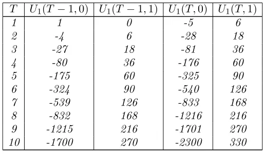
Corollary 2.22. Review identity (2.16) in sense of summation of D1(n, k) over some range W

with max(W) =T, then (2.16) returns

X

1≤k≤T

D1(n, k) =U1(T,0)n0−U1(T,1)n1,

where T = 1,2,3, ...,N. By property (2.9) we rewrite above expression as

X

0≤k≤T−1

D1(n, k) =U1(T −1,0)n0−U1(T−1,1)n1

T U1(T −1,0) U1(T−1,1) U1(T,0) U1(T,1)

1 1 0 -5 6

2 -4 6 -28 18

3 -27 18 -81 36

4 -80 36 -176 60

5 -175 60 -325 90

6 -324 90 -540 126

7 -539 126 -833 168

8 -832 168 -1216 216

9 -1215 216 -1701 270

10 -1700 270 -2300 330

Table 5. Table of coefficientsU1(T−1,0), U1(T −1,1), U1(T,0), U1(T,1)given T = 1, ...,10.

Therefore, for every integer n≥1, T =n,

∀T =n: n3 =

(

U1(T,0)n0−U1(T,1)n1,

U1(T−1,0)n0−U1(T −1,1)n1.

Coefficients|U1(T−1,1)|are terms of sequence A028896 in OEIS, [23]. Coefficients|U1(T,0)|are

terms of sequence A275709 in OEIS, [20].

In this section we have derived a binomial distributed triangle (2.14), such that perfect cube

n could be found as sum of n-th row terms of triangle (2.14) over k, in ranges 1 ≤ k ≤ n or 0≤k≤n−1, wherenis natural. Therefore, the follow question is stated:

Question 2.23. Is there a generalization of A287326 in order to receive monomial nt, t > 3 as sum of n-th row terms of corresponding triangle, where t is natural?

3. Generalization of sequence A287326

In order to get analogs of Triangle (2.14) one should solve a system of equations, where unknowns are coefficients of polynomial and variable of polynomial is k(n−k). Triangle (2.14) is generated by polynomialD1(n, k), n≥0, 0≤k≤n, defined by (2.12). Here, let derive a triangle generated by polynomial D2(n, k), n ≥ 0, 0 ≤ k ≤ n, such that sum of n-th row terms over k, in ranges 1≤k≤nor 0≤k≤n−1 returnsn5, wheren is natural

Example 3.1. We suspect thatn-th row of triangle that returnsn5as sum ofn-th row terms over

k, in 1≤k≤nor 0≤k≤n−1 is generated by

(3.2) D2(n, k) =A2,2(n−k)2k2+A2,1(n−k)1k1+A2,0(n−k)0k0, n≥0, 0≤k≤n,

whereA2,2, A2,1, A2,0 are unknown coefficients. Assume that for every integern≥0 holds

(3.3) n5 = X

1≤k≤n

To determine the coefficients A2,2, A2,1, A2,0, in (3.2) let rewrite (3.3) in extended view

A2,2

X

1≤k≤n

k2(n−k)2+A2,1

X

1≤k≤n

k(n−k) + X 1≤k≤n

A2,0 (3.4)

= A2,2

X

1≤k≤n

k2(n2−2nk+k2) +A2,1

X

1≤k≤n

kn−k2+ X 1≤k≤n

A2,0

= A2,2

X

1≤k≤n

k2n2−2nk3+k4+A2,1

X

1≤k≤n

kn−k2+ X 1≤k≤n

A2,0

= A2,2n2

X

1≤k≤n

k2−2A2,2n

X

1≤k≤n

k3+A2,2

X

1≤k≤n

k4+A2,1n

X

1≤k≤n

k

− A2,1

X

1≤k≤n

k2+ X 1≤k≤n

A2,0=n5.

Thus, we have received expression containing sums of powers of successive natural numbers, where powers are {1,2,3,4}. These formulas contain so-called Bernoulli numbers, [14]. For mentioned powers of successive natural numbers formulas are following

X

1≤k≤n

k= n 2_+n

2 , (3.5)

X

1≤k≤n

k2 = 2n

3_{+ 3n}2_+n

6 ,

(3.6)

X

1≤k≤n

k3 = n

4_{+ 2n}3_+n2

4 ,

(3.7)

X

1≤k≤n

k4 = 6n

5_{+ 15n}4_{+ 10n}3_−n

30 .

(3.8)

Now we substitute above identities to (3.4), respectively,

A2,2n2

2n3+ 3n2+n

6 − 2A2,2n

n4+ 2n3+n2

4 +A2,2

6n5+ 15n4+ 10n3−n

30

+ A2,1n

n2+n

2 −A2,1

2n3+ 3n2+n

6 +A2,0n

Particularizing the elements of above expression and moving them under the common divisor, we get

(3.9) A2,2n

5_−A

2,2n+ 30A2,0

30 +A2,1

n3_−n 6

We have to remember that expression (3.9) is the left side of the input equation (3.3). Therefore,

(3.10) n5 = A2,2n 5_−A

2,2n+ 30A2,0

30 +A2,1

n3_−n 6

In order to satisfy (3.10) for each natural n, coefficients A2,0, A2,1, A2,2 should be a solutions of following system of equations



 

 

1

30A2,2 = 1

A2,1 = 1

The only solution of above system is A2,2 = 30, A2,1 = 0, A2,0 = 1. Hereby, polynomialD2(n, k) takes the form

(3.11) D2(n, k) =A2,2(n−k)2k2+A2,1(n−k)1k1+A2,0(n−k)0k0 = 30k2(n−k)2+ 1

And for every natural n≥1 holds

n5 = X

1≤k≤n

D2(n, k) =

X

1≤k≤n

30k2(n−k)2+ 1 (3.12)

= X

0≤k≤n−1

D2(n, k) =

X

0≤k≤n−1

30k2(n−k)2+ 1

Let show few initial rows of triangle built by D2(n, k), that is analog of triangle (2.14), which returns monomial n5 as sum ofn-th row terms over k, as 1≤k≤nor 0≤k≤n−1, by means of its symmetry

(3.13)

1

1 1

1 31 1

1 121 121 1

1 271 481 271 1

1 480 1081 1081 481 1

Figure 6. Triangle generated by polynomial D2(n, k), n≥0, 0≤k≤n, sequence A300656 in OEIS, [15].

Similarly, finding the coefficientsA3,0, A3,1, A3,2, A3,3 in

(3.14) D3(n, k) =A3,3k3(n−k)3+A3,2k2(n−k)2+A3,1k1(n−k)1+A3,0k0(n−k)0,

we getA3,3= 140, A3,2 =−14, A3,1= 0, A3,0= 1, therefore, for each integer n≥0 holds

n7 = X

1≤k≤n

D3(n, k) =

X

1≤k≤n

140k3(n−k)3−14k2(n−k)2+ 1 (3.15)

= X

0≤k≤n−1

D3(n, k) =

X

0≤k≤n−1

140k3(n−k)3−14k2(n−k)2+ 1

Below we show a few initial rows of triangle generated by polynomial D3(n, k), n≥0, 0≤k≤n, the analog of triangle (2.14), such that monomialn7 could be found as sum ofn-th row terms over

k, as 1≤k≤nor 0≤k≤n−1, by means of its symmetry

(3.16)

1

1 1

1 127 1

1 1093 1093 1

1 3793 8905 3793 1

1 8905 30157 30157 8905 1

We assume now that generalization of A287326 holds for odd powers of the form 2m+ 1, m = 0,1,2, ..., where A287326 is partial case form= 1. To generalize our sequences A287326, A300656, A300785 for every odd power 2m+1, m≥0 one has to review the generating functions of sequences A287326, A300656, A300785 as follows. Let be definition

Definition 3.17.

Dm(n, k) := Am,mkm(n−k)m+Am,m−1km−1(n−k)m−1+· · ·+Am,0k0(n−k)0

= X

0≤j≤m

Am,jkj(n−k)j,

whereAm,j, 0≤j≤m are unknown coefficients. And, we assume that

(3.18) n2m+1 = X

1≤k≤n

Dm(n, k).

We want to notice that as we used a compact sigma notation on definition (3.17), i.e we rewrite (3.17) as P

0≤j≤mAm,jkj(n−k)j, thus the sum (3.18) returns indeterminate form of Dm(n, k) =

P

0≤j≤mAm,jkj(n−k)j on step k=nas Am,0(n−n)0k0 contains the term (n−n)0 = 00. Some textbooks leave the quantity 00 undefined, because the functions x0 and 0x have different limiting values whenx decreases to 0. But this is a mistake. We must define

∀x: x0= 1,

if the binomial theorem is to be valid when x = 0, y = 0, and/or x = y. The binomial theorem is too important to be arbitrarily restricted! By contrast, the function 0x _{is quite unimportant,} [31]. Note that Dm(n, k) is generalization of (2.12) and (3.11). For example, generating functions of sequences A287326, A300656, A300785 are, respectively



 

 

D1(n, k) = 1 + 6k(n−k), forA287326

D2(n, k) = 1−0k(n−k) + 30k2(n−k)2, forA300656

D3(n, k) = 1−14k(n−k) + 0k2(n−k)2+ 140k3(n−k)3, forA300785

Where coefficientsAm,j, form= 1,2,3 are{A1,j}1j=0={1,6}, {A2,j}2j=0 ={1,0,30}, {A3,j}3j=0=

{1,−14,0,140}in definitions of generating functions of A287326, A300656, A300785. To generalize above result in order to receive monomial n2m+1 asP

1≤k≤nDm(n, k) =n2m+1, m= 0,1,2, ...one has to solve the system of equations. Complete set of coefficients {Am,0, . . . , Am,m} such that

P

1≤k≤nDm(n, k) =n2m+1, m≥0 holds can be found by solving the following system of equations

(3.19)



      

      

Dm(1,0) = 12m+1

Dm(2,0) +Dm(2,1) = 22m+1

Dm(3,0) +Dm(3,1) +Dm(3,2) = 32m+1 ..

.

Dm(r,0) +Dm(r,1) +· · ·+Dm(r, r−1) =r2m+1, r > m

List of solutions1 of system (3.19) is split and assigned to OEIS under the numbers A302971 (numerators of Am,j) and A304042 (denominators of Am,j). To reach recurrent formula of Am,j,

first let fix the unused values Am,j = 0, for j < 0 or j > m, so we don’t need to care about the summation range forj, then by expanding (n−k)j and using Faulhaber’s formula [7], we get

n−1

X

k=0

(n−k)jkj = n−1

X k=0 ∞ X i j i

nj−i(−1)iki+j

(3.20) = ∞ X i j i

nj−i (−1)

i

i+j+ 1

"_∞

X

t

i+j+ 1

t

Btni+j+1−t−Bi+j+1

# = ∞ X i,t j i

(−1)i

i+j+ 1

i+j+ 1

t

Btn2j+1−t

| {z }

(?) − ∞ X i j i

(−1)i

i+j+ 1Bi+j+1n j−i

| {z }

()

whereBt are Bernoulli numbers [14]. Now, we notice that

(3.21) ∞ X i j i

(−1)i

i+j+ 1

i+j+ 1

t =    1 (2j+1)(2j

j)

, ift= 0;

(−1)j

t j 2j−t+1

, ift >0

In particular, the last sum is zero for 0< t≤j. Now we revise the (?) part of (3.20) according to results of (3.21), thus

∞ X i,t j i

(−1)i

i+j+ 1

i+j+ 1

t

Btn2j+1−t =

1 (2j+ 1) 2j_j

+ X t>0

(−1)j

t

j

2j−t+ 1

Btn2j+1−t

Therefore, (3.20) takes the form

n−1

X

k=0

(n−k)jkj = 1

(2j+ 1) 2j_j + X

t>0 (−1)j

t

j

2j−t+ 1

Btn2j+1−t

| {z }

(?) (3.22) − ∞ X i j i

(−1)i

i+j+ 1Bi+j+1n j−i

| {z }

()

Now, we keep our attention to (3.22) and we have to remember that if the sum over some variablei

contains j_i, then instead of limiting its summation range toi= 0, ..., j, we can leti=−∞, ...,+∞

respectively, we get n−1

X

k=0

(n−k)jkj = 1 (2j+ 1) 2j_jn

2j+1₊

∞ X

`=−∞

(−1)j 2j+ 1−`

j `

B2j+1−`n` (3.23)

− ∞ X

`=−∞

j `

(−1)j−`

2j+ 1−`B2j+1−`n

`

= 1

(2j+ 1) 2j_jn

2j+1_{+ 2}

∞ X

odd`

(−1)j 2j+ 1−`

j `

B2j+1−`n`.

Now, using the definition ofAm,j, we obtain the following identity for polynomials in n

∞ X

j

Am,j 1

(2j+ 1) 2j_jn

2j+1_{+ 2}

∞ X

j,odd`

Am,j

j `

(−1)j

2j+ 1−`B2j+1−`n

` (3.24)

≡n2m+1.

Taking the coefficient ofn2m+1 in above expression, we get Am,m = (2m+ 1) 2m_m

,and taking the coefficient of x2d+1 for an integer d in the range m/2 ≤ d < m we get Am,d = 0. Taking the coefficient ofn2d+1 in (3.24) for m/4≤d < m/2 , we get

(3.25) Am,d 1

(2d+ 1) 2d_d + 2(2m+ 1)

2m m

m

2d+ 1

(−1)m

2m−2dB2m−2d= 0,

i.e

(3.26) Am,d = (−1)m−1

(2m+ 1)!

d!d!m!(m−2d−1)! 1

m−dB2m−2d.

Continue similarly, we can expressAm,j for each integerj in range m/2s+1 ≤j < m/2s (iterating consecutively s= 1,2, ...) via previously determined values ofAm,d, d < j as follows

(3.27) Am,j = (2j+ 1)

2j j

m

X

d=2j+1

Am,d

d

2j+ 1

(−1)d−1

d−j B2d−2j.

The same formula holds also form= 0. Note that in above summhave to bem≥2j+ 1 to return nonzero termAm,j.

Definition 3.28. We define here a generating function of sequence of coefficientsAm,j, such that

Pn−1

k=0Dm(n, k) =n2m+1, n≥0, m≥0, whereDm(n, k) is defined by (3.17)

Am,j :=



 

 

0, if j <0 or j > m

(2j+ 1) 2j_j Pm

d=2j+1Am,d _2j+1d

(−1)d−1

d−j B2d−2j, if 0≤j < m (2j+ 1) 2j_j

, if j=m

Five initial rows of triangle generated byAm,j, j ≥0, 0≤j≤m are

(3.29)

m= 0 1

m= 1 1 6

m= 2 1 0 30

m= 3 1 -14 0 140

m= 4 1 -120 0 0 630

Figure 8. Triangle generated byAm,j, j ≥0, 0≤j≤m, sequences A302971 (numerators of

Am,j) and A304042 (denominators ofAm,j).

Note that starting from row m ≥ 11 the terms of Triangle (3.29) consist fractional numbers, for example,A11,1= 800361655623,6. One can find complete list of the numerators and denominators of Am,j in OEIS under the identifiers A302971 and A304042, respectively, see [17],[18]. To verify the terms that definition (3.28) produces one should refer to Mathematica code2. Hereby, let be theorem

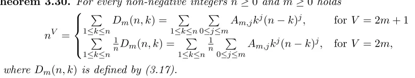
Theorem 3.30. For every non-negative integersn≥0 and m≥0 holds

nV =



 

 

P

1≤k≤n

Dm(n, k) = P 1≤k≤n

P

0≤j≤m

Am,jkj(n−k)j, forV = 2m+ 1

P

1≤k≤n 1

nDm(n, k) =

P

1≤k≤n 1 n

P

0≤j≤m

Am,jkj(n−k)j, forV = 2m,

where Dm(n, k) is defined by (3.17).

One can verify results concerning above theorem (3.30) via Mathematica code3. Therefore, theorem (3.30) answers to the question (2.23) positively, since for every m ≥ 0 exists a triangle, generated by Dm(n, k), n≥0, 0≤k ≤n, such that odd power n2m+1 can be reached as sum of

n-th row of corresponding triangle over 1≤k≤nor 0≤k≤n−1. Sequences A287326, A300656, A300785 are partial cases of theorem (3.30) for m= 1,2,3, respectively.

3.1. Properties of Dm(n, k) and Am,j. Here we show a few properties of definition Dm(n, k), some of them correlates with properties of partial case D1(n, k) in 2.15.

(1) Sum ofAm,j over j in range 0≤j ≤m gives

X

0≤j≤m

Am,j = 22m+1−1,

where Am,j is defined by (3.28).

(2) Similarly to property (2.21) of particular caseD1(n, k), items of{Dm(n, k)}nk=0, m≥0, n≥ 0 is symmetric, i.e

Dm(n, k) =Dm(n, n−k), for all k: 0≤k≤n.

(3) By property (2) for every integer n≥0, m≥0 immediately follows

n2m+1= X 1≤k≤n

Dm(n, k) = X 0≤k≤n−1

Dm(n, k)

(4) For everym≥0 the Am,m are terms of the sequence A002457, [19]. (5) For each m≥0

Am,0 = 1

(6) Assume that n <0, then theorem (3.30) can be applied as

nV =



 

 

P

1≤k≤|n|

Dm(n, k), forV = 2m+ 1

P

1≤k≤|n|

1

|n|Dm(|n|, k), forV = 2m

Property 3.31. (Linear Recurrence ofDm(n, k).) For every integern≥0 in D1(n, k), D2(n, k), D3(n, k) hold the recurrent relations

D1(n+ 1, k) = 2D1(n, k)−D1(n−1, k)

D2(n+ 2, k) = 3D2(n+ 1, k)−3D2(n, k) +D2(n−1, k)

D3(n+ 3, k) = 4D3(n+ 2, k)−6D3(n+ 1, k) + 4D3(n, k)−D3(n−1, k)

Review the coefficient Dm(n, k), which defined by m-order polynomial. It’s well known fact that

high order finite difference ∆m+kPm(x) = 0 for every x, where Pm(x) is m order polynomial and k >0,[8]. Recall Binomial Transform of sequencean. D. E. Knuth[35] has introduced the binomial

transform by

(3.32) aˆn=

n

X

k=0

n k

(−1)kak,

In particular, ˆan= ∆nan, therefore, for Dm(n, k) we have

(3.33) ∀t≥m: Dbm(n, k)t= X

j≥0

(−1)j

t+ 1

j

Dm(n+t−j, k)

≡0,

hereby, it gives us right to represent recursively every value of Dm(n+r, k), 0≤r≤t+ 1as

(3.34) (−1)r+1

t+ 1

r

Dm(n+t−r, k) =

X

j∈_Z≥0/{r}

(−1)j+1

t+ 1

j

Dm(n+t−j, k)

In particular,

(3.35) Dm(n+t, k) =

X

j≥1

(−1)j+1

t+ 1

j

Dm(n+t−j, k)

Hereby, let be theorem

Theorem 3.36. By property (3.31), particularly, from expression (3.35), for every integer t≥m follows

(3.37) (n+t)2m+1=X k≥1

X

j≥1

(−1)j+1

t+ 1

j

Dm(n+t−j, k)

Proof. Direct consequence of theorem (3.30) and (3.35).

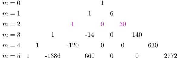
3.2. Example of use of theorem (3.30). In this subsection we show a detailed application of theorem (3.30). In this subsection we highlight the corresponding terms of Am,j, 0≤j ≤m and

T(n, k), 1≤k≤nwith different colors to be more easily to see regularity. Recall existing pattern, that is triangle of coefficientsAm,j defined by (3.28)

m= 0 1

m= 1 1 6

m= 2 1 0 30

m= 3 1 -14 0 140

m= 4 1 -120 0 0 630

m= 5 1 -1386 660 0 0 2772

By received formulaP

1≤k≤n

P

j≥0Dm(n, k) = n2m+1 each line of above triangle being multiplied by Tj>0(n, k) := kj(n−k)j and summed up to n or n−1 over k from 0 or 1, respectively, will result odd power of n2m+1, depending on the row Am,j, 0≤j ≤m is applied. Consider the case

n= 3, m= 2, we introduce triangle built using T(n, k) :=k(n−k), n ≥1, 1 ≤k≤n as upper triangular array, let be 1≤n≤5, 1≤k≤n

(3.38)

n= 1 n= 2 n= 3 n= 4 n= 5

0 1 2 3 4

0 2 4 6

0 3 6

0 4

0

Figure 10. Upper right triangle generated by T(n, k) =k(n−k), n≥1, 1≤k≤n, sequence A094053, [29] in OEIS.

Example 3.39. Consider theorem (3.30), let be n= 3 and m= 2, then

32·2+1 = 1·20+0·21+30·22

+ 1·20+0·21+30·22

+ 1·00+0·01+30·02

= 121 + 121 + 1 = 243

Items in above array are terms of the third row of triangle A300656.

Example 3.40. Consider theorem (3.30), let be n= 3 and m= 3, then 32·3+1 = 1·20−14·21+ 0·22+ 140·23

+ 1·20−14·21+ 0·22+ 140·23 + 1·00−14·01+ 0·02+ 140·03

= 1093 + 1093 + 1 = 2187

Items in above array are terms of the third row of triangle A300785.

Example 3.41. Consider theorem (3.30), let be n= 4 and m= 3, then 42·3+1 = 1·30−14·31+ 0·32+ 140·33

+ 1·40−14·41+ 0·42+ 140·43 + 1·30−14·31+ 0·32+ 140·33

+ 1·00−14·01+ 0·02+ 140·03 = 3739 + 8905 + 3739 + 1 = 16384

Items in above array are terms of the forth row of triangle A300785. We can perform same result for 42·3+1 in terms of multiplication of certain matrices,

42·3+1= [1,1,1,1]· 

  

30 31 32 33 40 ₄1 ₄2 ₄3 30 31 32 33 00 ₀1 ₀2 ₀3



   ·



  

1

−14 0 140



Example 3.42. Consider theorem (3.30), let be n= 5 and m= 3, then 52·3+1 = 1·40−14·41+ 0·42+ 140·43

+ 1·60−14·61+ 0·62+ 140·63 + 1·60−14·61+ 0·62+ 140·63 + 1·40−14·41+ 0·42+ 140·43

+ 1·00−14·01+ 0·02+ 140·03

= 8905 + 30157 + 30157 + 8905 + 1 = 78125

Items in above array are terms of the fifth row of triangle A300785.

Example 3.43. Consider theorem (3.30), let be n= 5 and m= 4, then 52·4+1 = 1·40−120·41+ 0·42+ 0·43+ 630·44

+ 1·60−120·61+ 0·62+ 0·63+ 630·64

+ 1·60−120·61+ 0·62+ 0·63+ 630·64 + 1·40−120·41+ 0·42+ 0·43+ 630·44 + 1·00−120·01+ 0·02+ 0·03+ 630·04

= 160801 + 815761 + 815761 + 160801 + 1 = 1953125

4. Another power identity

Review the Corollary (2.2), it says that partial case of theorem (3.30) returns the binomial of the form

X

M≤k≤N

D1(n, k) =

(

U1(T,0)n0+U1(T,1)n1, if M = 1, N =T

U1(T−1,0)n0+U1(T−1,1)n1, if M = 0, N =T −1

= n3, as T →n.

Let extend this idea, as we have complete theorem (3.30). We rewrite theorem (3.30) for odd powers as

X

M≤k≤N

Dm(n, k) =

(

Um(T,0)n0+· · ·+Um(T, m)nm, if M = 1, N =T

Um(T−1,0)n0+· · ·+Um(T −1, m)nm, if M = 0, N =T −1

= n2m+1, asT =n.

Above expression is so-called ’closed form’ of the theorem (3.30) for every particular n. Below we place a few examples of polynomialsP

0≤k≤m(−1)m

−k_{Um(T, k)·n}k_{, where m= 2,}

(4.1)

T U2(T,0)n0+U2(T,1)n1+U2(T,2)n2 1 31−60n+ 30n2

2 512−540n+ 150n2

3 2943−2160n+ 420n2

4 10624−6000n+ 900n2

5 29375−13500n+ 1650n2

6 68256−26460n+ 2730n2

7 140287−47040n+ 4200n2

8 263168−77760n+ 6120n2

9 459999−121500n+ 8550n2

Figure 11. Table of polynomials generated by P

1≤k≤T D2(n, k) =n5 asT →n, see definition (3.17) forD2(n, k).

Below we show a plots of few first polynomials P

1≤k≤T D2(n, k) for T = 1,2,3 and compare it with corresponding monomial n5 by the theorem (3.30),

31_-60_n+30_n2

512_-540_n+150_n2

2943_-2160_n+420_n2

n5

2 3 4 5

500 1000 1500 2000 2500 3000

Figure 12. Local approximations of monomial n5 by corresponding polynomials P

1≤k≤TD2(n, k) forT = 1,2,3, by theorem (3.30).

We can see that monomial n5 can be easily approximated in neighborhood of every particular natural n. The polynomials from figure (11) can be generated using Mathematica code4. To understand the nature of coefficientsUm(T, k), let derive them directly by means of theorem (3.30),

n

X

k=1 m

X

j=0

Am,jkj(n−k)j = n

X

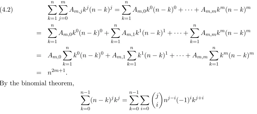
k=1

Am,0k0(n−k)0+· · ·+Am,mkm(n−k)m (4.2)

= n

X

k=1

Am,0k0(n−k)0+ n

X

k=1

Am,1k1(n−k)1+· · ·+ n

X

k=1

Am,mkm(n−k)m

= Am,0 n

X

k=1

k0(n−k)0+Am,1 n

X

k=1

k1(n−k)1+· · ·+Am,m n

X

k=1

km(n−k)m

= n2m+1.

By the binomial theorem, n−1

X

k=0

(n−k)jkj = n−1

X

k=0

X

i=0

j i

nj−i(−1)ikj+i

4_{Um(n,k) coefficients2.txt. - Mathematica code, generates the polynomials from figure (11), [39]. If necessary, one}

We rewrite the main result of (4.2) as

Am,0 n

X

k=1

k0(n−k)0+Am,1 n

X

k=1

k1(n−k)1+· · ·+Am,m n

X

k=1

km(n−k)m (4.3)

= Am,0 n X k=1 X i=0 0 i

n0−i(−1)ik0+i+Am,1 n X k=1 X i=0 1 i

n1−i(−1)ik1+i

+ Am,2 n X k=1 X i=0 2 i

n2−i(−1)ik2+i+Am,3 n X k=1 X i=0 3 i

n3−i(−1)ik3+i

.. .

+ Am,m n X k=1 X i=0 m i

nm−i(−1)ikm+i =n2m+1

Rewrite expression (4.3) in extended view

Am,0 n

X

k=1

k0(n−k)0+Am,1 n

X

k=1

k1(n−k)1+· · ·+Am,m n

X

k=1

km(n−k)m (4.4)

= Am,0 n X k=1 0 0

n0(−1)0k0

+Am,1 n X k=1 1 0

n1(−1)0k1+

1 1

n0(−1)1k2

+ Am,2 n X k=1 2 0

n2(−1)0k2+

2 1

n1(−1)1k3+

2 2

n0(−1)2k4

+ Am,3 n X k=1 3 0

n3(−1)0k3+

3 1

n2(−1)1k4+

3 2

n1(−1)2k5+

3 3

n0(−1)3k6

.. .

+ Am,m n X k=1 m 0

nm(−1)0km+

m

1

nm−1(−1)1km+1+· · ·+

m m

n0(−1)mk2m

= n2m+1.

Let rewrite expression (4.4) again and move sigma notation under the brackets,

n2m+1=Am,0 n

X

k=1

k0(n−k)0 +· · ·+ Am,m n

X

k=1

km(n−k)m (4.5)

= Am,0

" _n X k=1 0 0

n0(−1)0k0

#

+Am,1

" _n X k=1 1 0

n1(−1)0k1+ n X k=1 1 1

n0(−1)1k2

#

+ Am,2

" _n X k=1 2 0

n2(−1)0k2+ n X k=1 2 1

n1(−1)1k3+ n X k=1 2 2

n0(−1)2k4

#

+ Am,3

" _n X k=1 3 0

n3(−1)0k3+ n X k=1 3 1

n2(−1)1k4+ n X k=1 3 2

n1(−1)2k5+ n X k=1 3 3

n0(−1)3k6

#

.. .

+ Am,m

" _n X k=1 m 0

nm(−1)0km+ n X k=1 m 1

nm−1(−1)1km+1+· · ·+ n X k=1 m m

n0(−1)mk2m

For example, consider the polynomialPm

k=0(−1)m−kUm(n, k)nk, wherem= 3. We derive below a set of coefficientsU3(n,0), U3(n,1), U3(n,2), U3(n,3)

3

X

k=0

(−1)3−kU3(n, k)nk (4.6)

≡ A3,0

" _n X k=1 0 0

n0(−1)0k0

#

+A3,1

" _n X k=1 1 0

n1(−1)0k1+ n X k=1 1 1

n0(−1)1k2

#

+ A3,2

" _n X k=1 2 0

n2(−1)0k2+ n X k=1 2 1

n1(−1)1k3+ n X k=1 2 2

n0(−1)2k4

#

+ A3,3

" _n X k=1 3 0

n3(−1)0k3+ n X k=1 3 1

n2(−1)1k4+ n X k=1 3 2

n1(−1)2k5+ n X k=1 3 3

n0(−1)3k6

#

≡ n7.

The coefficientsU3(n,0), U3(n,1), U3(n,2), U3(n,3) in expression (4.6) are following

U3(n,0) = A3,0 n X k=1 0 0

(−1)0k0+A3,1 n X k=1 1 1

(−1)1k2

(4.7)

+ A3,2 n X k=1 2 2

(−1)2k4+A3,3 n X k=1 3 3

(−1)3k6,

U3(n,1) = A3,1 n X k=1 1 0

(−1)0k1+A3,2 n X k=1 2 1

(−1)1k3

(4.8)

+ A3,3 n X k=1 3 2

(−1)2k5,

U3(n,2) = A3,2 n X k=1 2 0

(−1)0k2+A3,3 n X k=1 3 1

(−1)1k4

(4.9)

U3(n,3) = A3,3 n X k=1 3 0

(−1)0k3.

(4.10)

Let rewrite above identities in compact form as,

U3(n, r = 0) = 3

X

t≥0

Am,t n X `=1 t t

(−1)t`2t

(4.11)

= 3

X

t≥0 n X `=1 Am,t t t

(−1)t`2t

U3(n, r = 1) = 3

X

t≥1

Am,t n X `=1 t t−1

(−1)t−1`2t−1

= 3

X

t≥1 n X `=1 Am,t t t−1

(−1)t−1`2t−1

U3(n, r = 2) = 3

X

t≥2

Am,t n X `=1 t t−2

(−1)t−2`2t−2

(4.13)

= 3

X

t≥2 n X `=1 Am,t t t−2

(−1)t−2`2t−2

U3(n, r = 3) = 3

X

t≥3

Am,t n X `=1 t t−3

(−1)t−3`2t−3

(4.14)

= Am,3 n

X

`=1

3

t−3

(−1)0`3

Note that above compact forms are depend on r = 0,1,2,3, as it can be seen by corresponding binomial coefficients, thus we have replaced kby `, to avoid confusion in notations. Therefore, for every 0≤r ≤m theUm(n, r) can be defined next way

Um(n, r) def= m

X

t≥r

Am,t n X `=1 t t−r

(−1)t−r`2t−r

(4.15)

= m

X

t≥r n X `=1 Am,t t t−r

(−1)t−r`2t−r

Similarly, the coefficientsUm(n−1, r) derived just by changing the iteration limits within the sum

Pn

`=1Am,t t t−r

(−1)t−r`2t−r in (4.15) from`∈ {1, n} to`∈ {0, n−1}

Um(n−1, r) def= m

X

t≥r

Am,t n−1

X

`=0

t t−r

(−1)t−r`2t−r

(4.16)

= m

X

t≥r n−1

X

`=0

Am,t

t t−r

(−1)t−r`2t−r

In above equation (4.16) it must be defined`0 = 1 for all`, see [31]. Mathematica implementations 56_{of expessions (4.15) and (4.16) are available in [41], [42]. Therefore, for everyn≥1, andm≥0,}

we have identity

n2m+1 = X

0≤r≤m

(−1)m−rUm(n, r)·nr (4.17)

= X

0≤r≤m

(−1)m−rUm(n−1, r)·nr (4.18)

Expressions (4.17), (4.18) are analogs to Faulhaber’s odd power identity, see property (2.3) and [21], p. 9. Expressions (4.17), (4.18) could be verified via Mathematica codes 7 8. Here we’d like

5_{Um(n,k) coefficients row generating.txt. - Mathematica code, implementation of (4.15), prints ten initial rows of}

coefficientsUm(n, k)

6_{Um(n-1,k) coefficients row generating.txt. - Mathematica code, implementation of (4.16), prints ten initial rows of} coefficientsUm(n−1, k)

to show a few examples of polynomials generated by P

0≤k≤T−1D2(n, k), see definition (3.17) for

D2(n, k)

(4.19)

T U2(T −1,0)n0+U2(T−1,1)n1+U2(T−1,2)n2

1 1

2 32−60n+ 30n2

3 513−540n+ 150n2

4 2944−2160n+ 420n2

5 10625−6000n+ 900n2

6 29376−13500n+ 1650n2

7 68257−26460n+ 2730n2

8 140288−47040n+ 4200n2

9 263169−77760n+ 6120n2

10 460000−121500n+ 8550n2

Figure 13. Table of polynomials generated by P

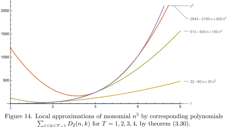
0≤k≤T−1D2(n, k). Below we show a plots of few first polynomials P

1≤k≤T−1D2(n, k) for T = 1,2,3,4 and compare it with corresponding monomialn5 by the theorem (3.30)

1

32_-60_n+30_n2

513_-540_n+150_n2

2944_-2160_n+420_n2

n5

2 3 4 5

500 1000 1500 2000

Figure 14. Local approximations of monomial n5 _{by corresponding polynomials}

P

1≤k≤T−1D2(n, k) for T = 1,2,3,4, by theorem (3.30).

The polynomials from figure (13) can be generated using Mathematica code9. Additionally, the generalized binomial series could be reached by means of identity

X

M≤k≤N

D1(n, k) =

(

U1(T,0)n0+U1(T,1)n1, if M = 1, N =T

U1(T−1,0)n0+U1(T−1,1)n1, if M = 0, N =T −1

= n3, as T →n.

For instance, for every naturaln

n3 =U1(T,0)·n0+U1(T,1)·n1

To reach higher powerm, let just multiply this identity bynm−3,

nm=U1(T,0)·nm−2+U1(T,1)·nm−3

9_{Um(n,k) coefficients.txt. - Mathematica code, generates the polynomials from figure (12), [40]. If necessary, one}

Let rewrite this expression regarding to itself as recursion,

nm = U1(T,0)·[U1(T,0)nm−4+U1(T,1)nm−5] +U1(T,1)·[U1(T,0)nm−5+U1(T,1)nm−6] = U1(T,0)2·nm−4−2·U1(T,0)·U1(T,1)nm−5+U1(T,1)2·nm−6

Repeating above process similarlyj ≥1 times, we have

nm = X

k≥0 (−1)k

j k

U1(T,0)j−k·U1(T,1)k·nm−2j−k (4.20)

= X k≥0

(−1)k

j k

U1(T−1,0)j−k·U1(T −1,1)k·nm−2j−k

We believe we can perform similarly in terms of multinomial coefficients,

nm = X

k1+k2+...+kt=j

j k1, k2, . . . , kt

t

Y

`=1

(−1)`Ut(T, `)k`·nm−(t+1)j−k (4.21)

= X

k1+k2+...+kt=j

j k1, k2, . . . , kt

t

Y

`=1

(−1)`Ut(T−1, `)k`_·nm−(t+1)j−k_.

Note that we must setT =nin above identities. Another way to represent odd-powered monomial

n2m+1, m = 0,1,2, ... is to define a polynomial U_m(n, k). As P

0≤k≤m(−1)m

−k_U

m(n, k)·nk =

P

0≤k≤m(−1)m

−k_{Um(n−1, k)·n}k_{, it follows that}

2n2m+1 = X 0≤k≤m

(−1)m−kUm(n, k)·nk+ X 0≤k≤m

(−1)m−kUm(n−1, k)·nk

= X

0≤k≤m

(−1)m−k(Um(n, k) +Um(n−1, k))·nk,

Let be definition

(4.22) U_m(n, k) def= 1 2

h

Um(n, k) +Um(n−1, k)

i

,

Therefore,

(4.23) n2m+1 = X

0≤k≤m

Um(n, k)·nk.

Expression (4.23) generates the following polynomials givenm= 2,

(4.24)

T U2(T,0)n0+U2(T,1)n1+U2(T,2)n2

1 16−30n+ 15n2

2 272−300n+ 90n2

3 1728−1350n+ 285n2

4 6784−4080n+ 660n2

5 20000−9750n+ 1275n2

6 48816−19980n+ 2190n2

7 104272−36750n+ 3465n2

8 201728−62400n+ 5160n2

9 361584−99630n+ 7335n2

10 610000−151500n+ 10050n2

Figure 15. Table of polynomials generated byP

Polynomials from Figure (15) could be generated using Mathematica code10. Let graphically show an approximation of monomialn5 _{by polynomials} P

0≤k≤mU2(T, k)·nk forT = 1,2,3,4.

16_-30_n+15_n2

272_-300n+90n2

1728_-1350_n+285_n2

6784_-4080_n+660_n2

n5

2 3 4 5 6

1000 2000 3000 4000 5000

Figure 16. Local approximations of monomial n5 by corresponding polynomials

P

0≤k≤mU2(T, k)·nk forT = 1,2,3,4.

Definition (4.22) of coefficients Um(n, k) and identity (4.23) could be verified via Mathematica codes 11 12, respectively. Similarly to (4.20), (4.21) we can perform a binomial and multinomial representation of monomialnm_{, wheren, m are non-negative integers andT =n,}

nm = X

k≥0 (−1)k

j k

U1(T,0)j−k· U1(T,1)k·nm−2j−k

(4.25)

= X k≥0

(−1)k

j k

U1(T−1,0)j−k· U1(T −1,1)k·nm−2j−k

And

nm = X

k1+k2+...+kt=j

j k1, k2, . . . , kt

t

Y

`=1

(−1)`Ut(T, `)k`_·nm−(t+1)j−k

(4.26)

= X

k1+k2+...+kt=j

j k1, k2, . . . , kt

t

Y

`=1

(−1)`U<sub>t</sub>(T −1, `)k`_·nm−(t+1)j−k_.

5. Acknowledgements

We would like to thank to Dr. Max Alekseyev (Department of Mathematics and Computational Biology, George Washington University) for sufficient help in deriving of Am,j coefficients, Dr. Hansruedi Widmer for useful comments concerning system of equations (3.19), Dr. Ron Knott (Visiting Fellow, Dept. of Mathematics at University of Surrey) for useful suggestions on writing of this article, and to Mr. Albert Tkaczyk for providing an analogs of triangle (2.14) for powers

m = 5,7, that are sequences A300656, A300785, respectively. Also, we’d like to thank to OEIS editors Michel Marcus, Peter Luschny, Jon E. Schoenfield and others for their patient and faithful volunteer work and for useful comments and suggestions during edition of sequences, concerned with this manuscript. We, also, thank to Tatyana Dryahlova for her help in translating of this manuscript in Russian.

10_{Combined U m(n,k) coefficients polynomials gf.txt. - Mathematica code, generates the polynomials from Figure}

(15), [43].

6. Conclusion

In this paper particular pattern, that is binomial distributed triangle A287326 in OEIS, which shows perfect cube n as sum of row terms over 0 ≤ k ≤ n−1 or 1 ≤ k ≤ n is generalized, in this manuscript are found and discussed the polynomialsDm(n, k) and Um(n, k), such that, when being summed up over k in some range with respect to m and n returns the monomial n2m+1. As first step, we discussed analogs of A287326 for powers l = 5,7, sequences A300656, A300785, respectively, then we derived coefficients Am,j, such that for everyn≥0 andm≥0 holds

n2m+1 = X 1≤k≤n

Dm(n, k),

where

Dm(n, k) :=Am,mkm(n−k)m+Am,m−1km−1(n−k)m−1+· · ·+Am,0k0(n−k)0,

and Am,j is defined by (3.28). Therefore, question question (2.23) is answered positively. Section (3) is totally dedicated to complete and extended derivation of identityP

1≤k≤nDm(n, k) =n2m+1. Properties of triangle (2.14) and polynomialDm(n, k) are shown in properties 2.15 and subsection 3.1, respectively. Relation between Faulhaber’s sumP

nmand finite differences of power are shown in 2.3. In section 4 we have generalized the main result of Corollary (2.2) for all odd powers of the form 2m+ 1, m= 0,1,2, ... and proven an identities

n2m+1 = X

0≤r≤m

(−1)m−rUm(n, r)·nr

= X

0≤r≤m

(−1)m−rUm(n−1, r)·nr.

References

[1] Conway, J. H. and Guy, R. K. ”Pascal’s Triangle.” In The Book of Numbers. New York: Springer-Verlag, pp. 68-70, 1996.

[2] Abramowitz, M. and Stegun, I. A. (Eds.). Handbook of Mathematical Functions with Formulas, Graphs, and Mathematical Tables, 9th printing. New York: Dover, pp. 10, 1972.

[3] Arfken, G. Mathematical Methods for Physicists, 3rd ed. Orlando, FL: Academic Press, pp. 307-308, 1985. [4] Weisstein, Eric W. ”Finite Difference.” From Mathworld.

[5] Weisstein, Eric W. ”Power.” From Mathworld.

[6] Richardson, C. H. An Introduction to the Calculus of Finite Differences. p. 5, 1954.

[7] Johann Faulhaber, Academia Algebræ, Darinnen die miraculosische Inventiones zuden h¨ochsten Cossen weiters continuirt und profitiert werden. Augspurg, bey Johann Ulrich Sch¨onigs, 1631. (Call number

QA154.8 F3 1631a f MATHat Stanford University Libraries.), online copy.

[8] Bakhvalov N. S. Numerical Methods: Analysis, Algebra, Ordinary Differential Equations p. 59, 1977. (In russian) [9] The OEIS Foundation Inc.,The On-Line Encyclopedia of Integer Sequences, 1964-present https://oeis.org/ [10] N. J. A. Sloane et al., Entry ”Coordination sequence for hexagonal lattice”, A008458 in [9], 2002-present. [11] Petro, Kolosov, et al., Entry ”Triangle read by rows: T(n, k) = 6∗(n−k)∗k+ 1”, A287326 in [9], 2017. [12] N. J. A. Sloane and Mira Bernstein et al., ”Pascal’s Triangle”, Entry A007318 in [9], 1994-present. [13] N. J. A. Sloane. ”Central polygonal numbers” Entry A000124 in [9], 1994-present.

[14] Weisstein, Eric W. ”Bernoulli Number.” From Mathworld–A Wolfram Web Resource.

[15] Petro, Kolosov, et al., Entry ”Triangle read by rows: T(n, k) = 30∗(n−k)2∗k2+ 1”, A300656 in [9], 2018. [16] Petro, Kolosov, et al., Entry ”Triangle read by rows: T(n, k) = 140∗(n−k)3_∗k3_{∗ −14∗(n−k)∗k+ 1”, A300785}

in [9], 2018.

[17] Petro, Kolosov, et al., Entry ”Triangle read by rows: Numeator(Am,j), 0≤j≤m, m≥0”, A302971 in [9], 2018.

[18] Petro, Kolosov, et al., Entry ”Triangle read by rows: Denominator(Am,j), 0≤j≤m, m≥0”, A304042 in [9], 2018.

[19] N. J. A. Sloane, et al., Entry ”a(n) = (2n+ 1)!/n!2”, A002457 in [9].

[21] Donald E. Knuth., Johann Faulhaber and Sums of Powers, pp. 9-10., arXiv preprint, arXiv:math/9207222v1 [math.CA], 1992.

[22] John Riordan, Combinatorial Identities (New York: John Wiley & Sons, 1968).

[23] Joe Keane, et al., Entry ”6 times triangular numbers: a(n) = 3∗n∗(n+ 1)”, A028896 in [9], 1999. [24] Mathematica code, provides the list of solutions of system (3.19) up tor= 11

https://kolosovpetro.github.io/mathematica codes/solutions system 2 4.txt

[25] Mathematica code, implementation of definition (3.28)

https://kolosovpetro.github.io/mathematica codes/def 2 12.txt

[26] Mathematica code, implementation of theorem (3.30)

https://kolosovpetro.github.io/mathematica codes/expression 2 1.txt

[27] Petro Kolosov, Peter Luschny, Entry ”Triangle read by rows: coefficients in the sum of odd powers as expressed by Faulhaber’s theorem,T(n, k) forn≥1,1≤k≤n”, A303675 in [9], 2018.

[28] Donald E. Knuth., Two notes on notation., pp. 1-2, arXiv preprint, arXiv:math/9205211 [math.HO], 1992. [29] Reinhard Zumkeller, et al., Entry ”Triangle read by rows: T(n, k) =k(n−k),1≤k≤n.”, A094053 in [9], 2004. [30] Early, Nick., Combinatorics and Representation Theory for Generalized Permutohedra I: Simplicial Plates., p.

3, arXiv preprint, arXiv:1611.06640 [math.CO], 2016.

[31] Ronald Graham, Donald Knuth, and Oren Patashnik (1989-01-05). ”Binomial coefficients”. Concrete Mathe-matics (1st ed.). Addison Wesley Longman Publishing Co. p. 162. ISBN 0-201-14236-8, online copy.

[32] Anggoro, A.; Liu, E.; and Tulloch, A. ”The Rascal Triangle.” College Math. J. 41, 393-395, 2010., online copy. [33] Clark Kimberling., Entry ”The Rascal Triangle ”, A077028 in [9], 2002-present.

[34] Worpitzky, J.. ”Studien uber die Bernoullischen und Eulerschen Zahlen..” Journal fur die reine und angewandte Mathematik 94 (1883): 203-232. http://eudml.org/doc/148532.

[35] Donald E. Knuth, The Art of Computer Programming Vol. 3, (1973) Addison-Wesley, Reading, MA.

[36] Agoh, Takashi, and Karl Dilcher. ”Generalized convolution identities for Stirling numbers of the second kind.” Integers 8.1 (2008): Article-A25, online copy.

[37] Mathematica code, implementation of (4.17),

https://kolosovpetro.github.io/mathematica codes/Um(n,k) odd power identity.txt.

[38] Mathematica code, implementation of (4.18),

https://kolosovpetro.github.io/mathematica codes/Um(n,k) odd power identity2.txt.

[39] Mathematica code, generates the polynomials from figure (11),

https://kolosovpetro.github.io/mathematica codes/Um(n,k) coefficients.txt.

[40] Mathematica code, generates the polynomials from figure (12),

https://kolosovpetro.github.io/mathematica codes/Um(n,k) coefficients2.txt.

[41] Mathematica code, implementation of (4.15), prints ten initial rows of coefficientsUm(n, k),

https://kolosovpetro.github.io/mathematica codes/Um(n,k) coefficients row generating.txt.

[42] Mathematica code, implementation of (4.16), prints ten initial rows of coefficientsUm(n−1, k),

https://kolosovpetro.github.io/mathematica codes/Um(n-1,k) coefficients row generating.txt.

[43] Mathematica code, generates the polynomials from Figure (15),

https://kolosovpetro.github.io/mathematica codes/Combined U m(n,k) coefficients polynomials gf.txt.

[44] Mathematica code, verifies the values definition (4.22) produces,

https://kolosovpetro.github.io/mathematica codes/Combined U m(n,k) coefficients gf.txt.

[45] Mathematica code, verifies identity (4.23),

https://kolosovpetro.github.io/mathematica codes/Combined U m(n,k) coefficients odd power identity.txt.

7. Application 1. Extended tables of polynomials, consisting Um(n, k) coefficients In this application we attach an extended table, consisting of polynomials, generated byP

1≤k≤TDm(n, k) and P

0≤k≤T−1Dm(n, k) for various t and m. We begin from cases m = 2,3,4 given generating functionP

1≤k≤T Dm(n, k) and continue similarly with examples forP0≤k≤T−1Dm(n, k). The fol-lowing tables could be generated using Mathematica code Um(n,k) coefficients2.txt. Here we begin to show our tables form= 1,2,3,4 andT = 1,2, ...,40

t Polynomial(n) 1 31−60n+ 30n2

2 512−540n+ 150n2

5 29375−13500n+ 1650n2

6 68256−26460n+ 2730n2

7 140287−47040n+ 4200n2

8 263168−77760n+ 6120n2

9 459999−121500n+ 8550n2 10 760000−181500n+ 11550n2

11 1199231−261360n+ 15180n2 12 1821312−365040n+ 19500n2

13 2678143−496860n+ 24570n2

14 3830624−661500n+ 30450n2

15 5349375−864000n+ 37200n2

16 7315456−1109760n+ 44880n2

17 9821087−1404540n+ 53550n2

18 12970368−1754460n+ 63270n2

19 16879999−2166000n+ 74100n2

20 21680000−2646000n+ 86100n2

21 27514431−3201660n+ 99330n2

22 34542112−3840540n+ 113850n2

23 42937343−4570560n+ 129720n2

24 52890624−5400000n+ 147000n2

25 64609375−6337500n+ 165750n2

26 78318656−7392060n+ 186030n2 27 94261887−8573040n+ 207900n2

28 112701568−9890160n+ 231420n2 29 133919999−11353500n+ 256650n2

30 158220000−12973500n+ 283650n2

Figure 17. Table for m= 2, generating function: P

1≤k≤T Dm(n, k) over T = 1,2, ...,30.

t Polynomial(n)

1 −125 + 406n−420n2+ 140n3

2 −9028 + 13818n−7140n2+ 1260n3

3 −110961 + 115836n−41160n2+ 5040n3

4 −684176 + 545860n−148680n2+ 14000n3

5 −2871325 + 1858290n−411180n2+ 31500n3

6 −9402660 + 5124126n−955500n2+ 61740n3

7 −25872833 + 12182968n−1963920n2+ 109760n3

8 −62572096 + 25945416n−3684240n2+ 181440n3

9 −136972701 + 50745870n−6439860n2+ 283500n3

10 −276971300 + 92745730n−10639860n2+ 423500n3

11 −524988145 + 160386996n−16789080n2+ 609840n3

12 −943023888 + 264896268n−25498200n2+ 851760n3

13 −1618774781 + 420839146n−37493820n2+ 1159340n3

14 −2672907076 + 646725030n−53628540n2_{+ 1543500n}3 15 −4267591425 + 965662320n−74891040n2+ 2016000n3

16 −6616398080 + 1406064016n−102416160n2_{+ 2589440n}3 17 −9995653693 + 2002403718n−137494980n2+ 3277260n3

18 −14757360516 + 2796022026n−181584900n2+ 4093740n3

19 −21343778801 + 3835983340n−236319720n2+ 5054000n3

21 −42311023965 + 6895305186n−385201740n2+ 7470540n3

22 −58184203748 + 9059830318n−483589260n2+ 8961260n3

23 −78909220801 + 11763094056n−601122480n2+ 10664640n3

24 −105663629376 + 15107395800n−740468400n2+ 12600000n3

25 −139843308125 + 19208957950n−904530900n2_{+ 14787500n}3 26 −183091507300 + 24199135506n−1096460820n2+ 17248140n3

27 −237330365553 + 30225676068n−1319666040n2_{+ 20003760n}3 28 −304794997136 + 37454030236n−1577821560n2+ 23077040n3

29 −388070250301 + 46068712410n−1874879580n2+ 26491500n3

30 −490130237700 + 56274711990n−2215079580n2+ 30271500n3

31 −614380739585 + 68298954976n−2602958400n2+ 34442240n3

32 −764704580608 + 82391815968n−3043360320n2+ 39029760n3

33 −945510081021 + 98828680566n−3541447140n2+ 44060940n3

34 −1161782683076 + 117911558170n−4102708260n2+ 49563500n3

35 −1419139853425 + 139970745180n−4732970760n2+ 55566000n3

36 −1723889362320 + 165366538596n−5438409480n2+ 62097840n3

37 −2083091040413 + 194491000018n−6225557100n2+ 69189260n3

38 −2504622113956 + 227769770046n−7101314220n2+ 76871340n3

39 −2997246219201 + 265663933080n−8072959440n2+ 85176000n3

40 −3570686196800 + 308671932520n−9148159440n2+ 94136000n3

Figure 18. Form= 3, generating function: P

1≤k≤T Dm(n, k) over T = 1,2, ...,40.

t Polynomial(n)

1 751−2640n+ 3780n2−2520n3+ 630n4

2 162512−325440n+ 245700n2−83160n3+ 10710n4

3 4297023−5837040n+ 3001320n2−695520n3+ 61740n4

4 45586624−47125200n+ 18484200n2_−3276000n3_{+ 223020n}4 5 291683375−244000800n+ 77546700n2−11151000n3+ 616770n4

6 1349845776−949440240n+ 253906380n2_−30746520n3_{+ 1433250n}4 7 4981676287−3024769440n+ 698619600n2−73100160n3+ 2945880n4

8 15551330048−8309593440n+ 1689523920n2−155675520n3+ 5526360n4

9 42670773999−20362676400n+ 3698370900n2−304479000n3+ 9659790n4

10 105670786000−45562677600n+ 7478370900n2−556479000n3+ 15959790n4

11 240716895551−94670349840n+ 14174871480n2−962327520n3+ 25183620n4

12 511605381312−184966507440n+ 25461891000n2−1589384160n3+ 38247300n4

13 1025515755823−343092771840n+ 43707229020n2−2525042520n3+ 56240730n4

14 1955262884624−608734803600n+ 72168875100n2−3880359000n3+ 80442810n4

15 3569884005375−1039300430400n+ 115225437600n2−5793984000n3+ 112336560n4

16 6275713432576−1715757781440n+ 178643314080n2−8436395520n3+ 153624240n4

17 10670440655087−2749811239440n+ 269883324900n2−12014435160n3+ 206242470n4

18 17613015856848−4292605722240n+ 398449531620n2−16776146520n3+ 272377350n4

19 28312660615999−6545162506800n+ 576282961800n2−23015916000n3+ 354479580n4

20 44440660664000−9770762509200n+ 818202961800n2−31079916000n3+ 455279580n4

21 68269062114351−14309505635040n+ 1142398899180n2_{−41371850520n}3_{+ 577802610n}4 22 102840862500112−20595287515440n+ 1570974936300n2−54359003160n3+ 725383890n4

23 152176783290623−29175447644640n+ 2130550596720n2_{−70578587520n}3_{+ 901683720n}4 24 221524231290624−40733355636000n+ 2852919846000n2−90644400000n3+ 1110702600n4

25 317654602459375−56114215014000n+ 3775771408500n2−115253775000n3+ 1356796350n4

27 627146261293887−102714466735440n+ 6407922490200n2−181354088160n3+ 1979499060n4

28 865161520339648−136716646589040n+ 8229467839320n2−224724215520n3+ 2366732340n4

29 1180316760605999−180186334891200n+ 10477899992700n2−276412311000n3+ 2812319370n4

30 1593659760714000−235298734894800n+ 13233519992700n2−337648311000n3+ 3322619370n4

31 2130981114417151−304630522458240n+ 16588283906880n2_{−409793771520n}3_{+ 3904437600n}4 32 2823673440038912−391217063149440n+ 20647028001600n2−494350940160n3+ 4565040480n4

33 3709710869661423−498615539455440n+ 25528776924420n2_{−592972130520n}3_{+ 5312170710n}4 34 4834761029884624−630974381822400n+ 31368137616900n2−707469399000n3+ 6154062390n4

35 6253442526125375−793109409951600n+ 38316781679400n2−839824524000n3+ 7099456140n4

36 8030741767978176−990587103477840n+ 46545018909480n2−992199287520n3+ 8157614220n4

37 10243603824112687−1229815433857440n+ 56243464735500n2−1166946059160n3+ 9338335650n4

38 12982712871538448−1518142701993840n+ 67624804267020n2−1366618682520n3+ 10651971330n4

39 16354478705823999−1863964838829600n+ 80925655683600n2−1593983664000n3+ 12109439160n4

40 20483246706016000−2276841638834400n+ 96408535683600n2−1852031664000n3+ 13722239160n4

Figure 18. Form= 4, generating function: P

1≤k≤T Dm(n, k) over T = 1,2, ...,40. E-mail address: [email protected]