https://doi.org/10.5194/nhess-18-2273-2018 © Author(s) 2018. This work is distributed under the Creative Commons Attribution 4.0 License.
Estimating network related risks: A methodology and an
application in the transport sector
Jürgen Hackl1, Juan Carlos Lam1, Magnus Heitzler2, Bryan T. Adey1, and Lorenz Hurni2 1Institute of Construction and Infrastructure Management, ETH Zurich, 8092 Zurich, Switzerland 2Institute of Cartography and Geoinformation, ETH Zurich, 8092 Zurich, Switzerland
Correspondence:Jürgen Hackl ([email protected]) and Juan Carlos Lam ([email protected]) Received: 19 December 2017 – Discussion started: 2 January 2018
Revised: 16 July 2018 – Accepted: 31 July 2018 – Published: 27 August 2018
Abstract.Networks such as transportation, water, and power are critical lifelines for society. Managers plan and execute interventions to guarantee the operational state of their net-works under various circumstances, including after the oc-currence of (natural) hazard events. Creating an interven-tion program demands knowing the probable direct and in-direct consequences (i.e., risk) of the various hazard events that could occur in order to be able to mitigate their ef-fects. This paper introduces a methodology to support net-work managers in the quantification of the risk related to their networks. The methodology is centered on the inte-gration of the spatial and temporal attributes of the events that need to be modeled to estimate the risk. Furthermore, the methodology supports the inclusion of the uncertainty of these events and the propagation of these uncertainties throughout the risk modeling. The methodology is imple-mented through a modular simulation engine that supports the updating and swapping of models according to the needs of network managers. This work demonstrates the usefulness of the methodology and simulation engine through an appli-cation to estimate the potential impact of floods and mud-flows on a road network located in Switzerland. The applica-tion includes the modeling of (i) multiple time-varying haz-ard events; (ii) their physical and functional effects on net-work objects (i.e., bridges and road sections); (iii) the func-tional interrelationships of the affected objects; (iv) the re-sulting probable consequences in terms of expected costs of restoration, cost of traffic changes, and duration of network disruption; and (v) the restoration of the network.
1 Introduction
Managers of networks, such as transportation, water and power, have the continuous task to plan and execute inter-ventions to guarantee the operational state of their networks. This also applies in the aftermath of (natural) hazard events. As the resources available to managers to protect their net-works are limited, it is essential for managers to be aware of the probable consequences (i.e., risk) in order to set pri-orities and be resource-efficient (Eidsvig et al., 2017). Con-sequences are often expressed in monetary values, and these are distinguished between direct costs (e.g., costs related to clean up, repairs, rehabilitation and reconstruction) and in-direct costs (e.g., in the transport sector, costs related to ad-ditional travel time, vehicle operation and an increase in the number of accidents). Indirect costs have a wide spatial and temporal scale (Merz et al., 2010) and are potentially larger than direct costs (Vespignani, 2010).
net-work managers need to think of ways to model the cascade of events, interdependencies, and the propagation of uncer-tainties (Hackl et al., 2015).
As a result of these challenges, risk assessment methods for networks have been the subject of increasing research in-terest in recent years. Most research has been focused either on the technical aspects of hazards or those of networks. In the first case, scholars have focused on improving the un-derstanding, the modeling or the prediction of single haz-ard events (Apel et al., 2004; Pritchhaz-ard et al., 2015; Schlögl and Laaha, 2016; Pellicani et al., 2017) without explicitly considering the complexity and dynamics of networks. In the second case, scholars have investigated the vulnerabil-ity1 (Jenelius et al., 2006; Rupi et al., 2015; Shabou et al., 2017) or resilience (He and Liu, 2012; Bocchini and Fran-gopol, 2012; Vugrin et al., 2014) of networks due to disrup-tions, without evaluating the cause and/or the probability of such disruptions.
Some work has been conducted to consider multiple haz-ards and their effects (i.e., multiple vulnerabilities and con-sequences) in a unified framework (Komendantova et al., 2014; Mignan et al., 2014; Gallina et al., 2016). Assess-ing the risk in such a way is relatively new, and until now only partially developed by experts with different back-grounds such as statistics, engineering and various fields of geosciences (Komendantova et al., 2014). Only a limited number of scenario-based and/or site-specific studies have been proposed due to the difficulty and novelty of the task (Mignan et al., 2014). Having a diverse team of experts, whose discipline-specific approaches to risk assessment may differ, presents an additional challenge: their contributions are not always easy to aggregate to a level that is useful for network managers. In addition, current research also shows the need to take into account the spatial-temporal quantifica-tion of risks across different levels of scale for future sustain-able risk management (Fuchs and Keiler, 2008; Fuchs et al., 2013).
Open research. In conclusion, there has been little work to bring research outputs concerning the modeling of haz-ard events and network vulnerability together in a way that their spatial and temporal uncertain behaviors are assessed in a unified framework that fosters multidisciplinary collabora-tion.
Contributions. To overcome these challenges, this article presents the application of a novel risk assessment method-ology. The methodology can be used to investigate multiple scenarios, starting from the modeling of a source event (e.g., 1Numerous definitions for network vulnerability have been
pro-posed in the literature. In most cases, the literature has defined net-work vulnerability in terms of the effects of service disruption, irre-spective of its probability (Berdica, 2002; Taylor and D’Este, 2007; Wang et al., 2014). In the context of the present work, vulnerability is defined in the same terms, acknowledging that it is an inherent attribute of any network and thus an essential element of risk as-sessments.
rainfall, fault rupture), and ending in the estimation of the probable consequences of related societal events (e.g., com-munities without access to transportation, water or power ser-vice). While the methodology is applicable to different types of hazards, networks, regions, sizes of regions, and levels of resolution, the application of the methodology is illustrated on a regional road network in Switzerland prone to floods and mudflows. Specifically, this work advances the state-of-the-art in the field of network related risks due to hazard events as follows.
– The risk of a complete chain of events, from a source event to its societal events is quantified over space and time. In the application, this means considering pre-cipitation, runoff, flood, mudflows, (physical) damages, functional losses, traffic flow changes, and restoration interventions. The presented links between cascading hydrometeorological hazards, a road network and soci-ety will be of interest to the international research com-munity and practitioners working in the fields of net-work management, urban planning, public policy, and emergency response.
– When quantified, risk can be categorized into proba-ble direct and indirect costs, with the latter estimated throughout the hazard events and restoration periods, not just immediately after the occurrence of the haz-ard events. In the application, direct and indirect costs included costs of interventions, prolongation of travel time, and missed trips, allowing for the evaluation and comparison of the socio-economic impacts of the mul-tiple hazard scenarios considered.
– The simulation-based approach supports the inclusion of uncertainties and their propagation throughout the risk model. The application includes results related to the simulation of 1200 rainfall events, causing floods of return periods ranging from 2 to 10 000 and, depend-ing on the rainfall intensity and duration, stochastically triggering a number of mudflows in the area. Further-more, as suggested by Lam et al. (2018a), the approach can support the testing of additional scenarios based on uncertain relationships (e.g., fragility functions relating hazard intensities with damage state exceedance proba-bilities).
– A novel simulation engine was constructed as the com-putational platform to estimate risk, supporting the combination of models from different disciplines, and their modular update and replacement. The application demonstrates the coupling of existing models and in-formation from literature in geosciences, engineering, network theory, transportation, and economics.
the risk related to their networks due climate-related hazard events. With a changing climate, exacerbated by an increase in urbanization, the frequency of extreme hydrometeorolog-ical hazard events is expected to rise, impacting economic corridors, disrupting supply chain, and stressing emergency and rescue operations, among other effects (Keiler et al., 2010; Fuchs et al., 2017). As a result, special focus is now given to these hazard events and their associated risks. In times of scarce public resources and increasing incidences and damages caused by floods (Bowering et al., 2014), net-work managers have the need to become increasingly aware of their causes and consequences so that they can appropri-ately manage their risks, for example, through the adaptation of networks (Elsawah et al., 2014) or the planning of actions following a hazard event (Taubenböck et al., 2013). A num-ber of methods have been developed to quantify the damages and costs due to floods (Merz et al., 2010; Hammond et al., 2015). Nevertheless, most of these studies have been focused on buildings and the estimation of direct costs.
In the transport sector, some work has been done to con-sider the probable direct costs of floods (e.g., Scawthorn et al., 2006; Deckers et al., 2009; Bowering et al., 2014), but these works have often neglected the spatial and temporal attributes of these networks. Only a few scholars have in-vestigated flood risk in combination with the actual changes in traffic flow. Dawson et al. (2011) implemented an agent-based model to simulate the human response to floods con-sidering different storm surge conditions. Suarez et al. (2005) studied the impacts of floods and climate change on the ur-ban transport system of the Boston Metro Area, using a con-ventional analytical framework for simulating traffic flows under different flood scenarios, changes in land use, and de-mographic and climatic conditions. In both cases, the direct costs resulting from damages were not taken into account. Furthermore, only the events unfolding during the hazard events period were analyzed, and hence, no network restora-tion was considered, which is essential for quantifying indi-rect costs.
While floods are the most common rainfall-triggered haz-ard events in mountainous areas, landslides, including mud-flows, are second in place. As road networks in these areas generally have a low level of connectivity (e.g., remote vil-lages that are only connected by few mountain roads), there is a high probability that connections between some areas within a road network can be interrupted when one or a lim-ited number of objects fail (Rupi et al., 2015). Usually, risk estimates related to networks, including road networks, due to landslides have been obtained by overlapping hazard and consequence maps (Ferlisi et al., 2012; Pellicani et al., 2017) and thus the indirect costs for specific hazard scenarios have not been considered.
In general, according to Mattsson and Jenelius (2015), there are two dominant types of risk assessment methods for transport networks. The first set of methods is rooted in graph theory, and is focused on the study of the topological
prop-erties of the networks. This analytical approach requires net-work topology data and considers the importance of differ-ent edges (Jenelius et al., 2006; Rupi et al., 2015), cascad-ing failures (Dueñas-Osorio and Vemuru, 2009; Hackl and Adey, 2017), and interdependencies between different net-works (Thacker et al., 2017). The second group of methods is focused on understanding the dynamic behavior exhibited on networks (e.g., traffic flow) through the use of transporta-tion system models. While this approach has the potential to provide a more complete description of society-related con-sequences than graph-theory-based methods, the approach often requires extensive data and significant computational resources, limiting the modeling of this dynamic behavior to only a few deterministic scenarios.
This work is organized as follows. A brief overview of the risk assessment methodology is presented next in Sect. 2. Section 3 contains a description of the main features of the application to illustrate the use of the methodology. The re-sults obtained from the application are presented in Sect. 4 while a discussion about the findings, and the advantages and shortcomings of the methodology and the models used are given in Sect. 5. Concluding remarks and suggestions for future work are given in Sect. 6.
2 Risk assessment methodology
The purpose of the risk assessment methodology is to support network managers in the quantification and subsequent man-agement of risk. The methodology is founded on the princi-ples of systems engineering (Adey et al., 2016) and thus the methodology is structured keeping in mind that (i) different decisions require different models, (ii) models provide dif-ferent levels of detail, and (iii) this is an iterative process, requiring changes as data and model insufficiencies are dis-covered, and new data and models become available. Con-sidering these principles, the risk assessment methodology is structured as follows:
1. Set up risk assessment– the rough outline of the planned risk assessment.
2. Determine approach– the agreements on how to per-form the risk assessment, including the involved parties and the activities to conduct.
3. Define system representation– the agreements on sys-tem behavior, syssys-tem boundaries, assumptions and lim-itations.
– Define boundaries – the parts of the system to be analyzed, both spatially and temporally.
– Define events – the events to be analyzed.
– Define scenarios – the scenarios combining the events and relationships.
– Determine tools – the selection of tools, models and software to analyze the scenarios.
4. Estimate risk – the computed probabilities of the sce-narios and their consequences.
5. Evaluate risk– the interpretation of the risk estimates. 6. Update approach and/or system representation – the
parts of the system to be analyzed in more detail in order to decrease the uncertainties of the result.
The considered events are described using generic cate-gories: source, hazard, object, network and societal. Source events are ones that, at least from a modeling perspective, are considered to simply happen with a certain probability, and may lead to hazard events. Each object in the network is vulnerable to these hazard events, which may cause damage and/or functional losses. These impacts can be the origin of failures in the network resulting in a deficient level of ser-vice. These effects can impair the functioning of society dur-ing the hazard events and restoration periods. The execution of restoration interventions enables the network to provide an adequate level of service again by changing the state of damaged objects.
Such a chain of events can be assembled using a novel simulation engine (Heitzler et al., 2018) that supports the coupling of multiple heterogeneous models, where a given model encapsulates the behavior and state of a part of the sys-tem. To support the data exchange between models, models are grouped into modules, with each module comprising dis-tinct execution instructions and data requirements. The data consist of model parameters, static input (e.g., the location of mudflows, the extent of the road network, the distribu-tion of a variable to sample from) and the states of models in other modules (e.g., to determine the damaged objects, the water extend from a flood model is needed). The advantage of such a modular approach is that only input and output have to be defined for each module. Consequently, different mod-els and software solutions can be used to simulate scenar-ios. For example, a flood can be simulated using a custom model or off-the-shelf software such as HEC-RAS (Brunner, 2016), Basement (Vetsch et al., 2018), etc., without having to modify other models. This approach allows scientists to implement and test their own models, including their effects on risk estimations.
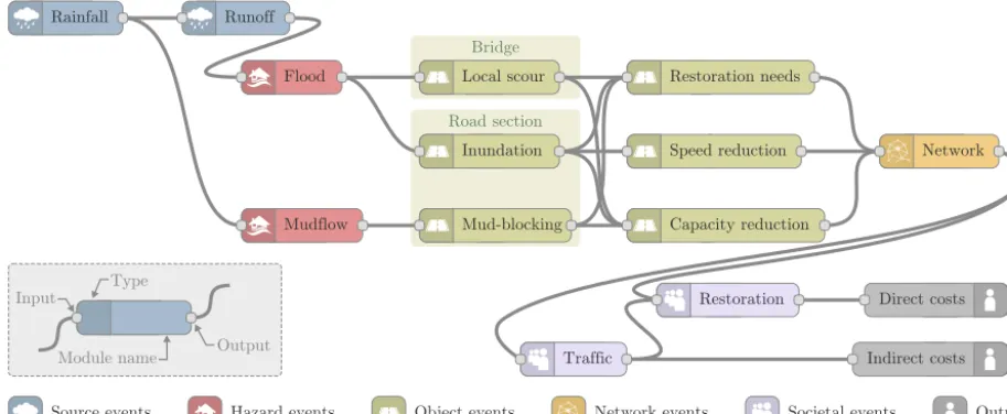
Once the modules and module interfaces are defined (as a reference, see Fig. 1 for a schematic representation of the modules used in the application), the network manager can conduct the risk assessment. Risk is here expressed in terms of expected monetized consequences, calculated as a prod-uct of the probability of occurrence of a certain scenario and the associated costs of that scenario – both the direct (dc) and the indirect costs (ic) should be considered. Their cost
functionsCdcandCicare associated with the modeled soci-etal eventsEsoc that occur as a result of object eventsEobj
and network eventsEnet, and that can be traced back to haz-ard eventsEhaz and source eventsEsrc. This representation (for a given source event, see Eq. 1) can also be used when considering multiple hazard events. As the spatial and tem-poral correlation between events is considered, risk can be said to be spatially and temporally distributed (i.e., risk es-timates vary in space within a defined area of study, and in time within a defined period of analysis).
R|Esrc=
probability
z }| {
P[Ehaz|Esrc]
·
consequences
z }| {
(Cdc(Esoc|Eobj, Ehaz)
| {z }
direct
+Cic(Esoc|Enet, Eobj, Ehaz)
| {z }
indirect
) (1)
Furthermore, network managers may be often interested in investigating the effect of hazard loads on their critical objects. Therefore, managers need to be given the option to select hazard events based on the periodicity of the mani-fested site-specific hazard loads (i.e., managers may not be as concerned with selecting a hazard event based on the re-turn period of the preceding source event). Then Eq. (1) can be modified by first selecting the hazard events according to the return periods related to the site-specific loads (i.e., risk is conditioned on the hazard event (R|Ehaz) and thus the proba-bility of occurrence of a scenario is defined asP[Esrc|Ehaz]). For example, the network manager might be interested to evaluate a flood with a return period of 100 years in a spe-cific point in the network. In this case, the simulation engine finds a suitable rainfall that causes the flood of interest.
3 Application
The application presented in this section is used to demon-strate the usefulness of the methodology considering a spe-cific problem. The application shows the design and imple-mentation of an assessment focused on estimating the risk related to a road network in the Canton of Grisons in Switzer-land. In the study, the network was exposed to rainfall, which caused multiple hazards, specifically riverine floods and mudflows. At the same time, these events led to direct costs linked to clean-up, repair, rehabilitation and reconstruc-tion activities, and indirect costs associated with loss of con-nectivity and temporal prolongation of network user travel time, linking the modeling of these latter effects with the dy-namics of the network. A large number of uncertain rainfall leading to floods of multiple return periods was considered in the analysis.
appli-Road section Bridge
Flood
Mudflow
Indirect costs Rainfall Runoff
Direct costs
Traffic
Restoration Mud-blocking
Inundation Local scour
Capacity reduction Speed reduction Restoration needs
Network
Outputs Source events Hazard events Object events Network events Societal events
Module name Type Input
Output
Figure 1.Schematic overview of the modules used for the application. Modules, represented by nodes with certain inputs and outputs, are related to the events that need to be modeled to estimate risk. The assessment starts with the modeling of a randomrainfalland its corre-spondingrunoff. Estimated discharge values at river stations of interest are used to simulate thefloodpropagation, including the inundation of the area. Amudflowcan be randomly triggered during the rainfall if accumulated precipitation values exceed certain thresholds. In the next step, expected damages (i.e.,bridge local scour,road section inundation,road section mud-blocking), functional losses (i.e.,speed reduction,capacity reduction), andrestoration needs(i.e., restoration cost, restoration time) are determined for each affected object in the network. The updated states of individual objects help define the new state of the entirenetwork. Thetrafficthrough the network is then simulated.Restorationinterventions are executed to enable the network to provide an adequate level of service again by changing the state of damaged objects. The costs for the restoration are accounted asdirect costs, while the costs related to additional vehicle travel time through the network and missed trips are accounted asindirect costs.
cation were chosen considering the need to keep the compu-tational time low. The authors of this paper are fully aware that other models may be available in the literature, some of which are more sophisticated and precise, and hence, demand much more detailed data than the data that were available. Nonetheless, the selection of data and models was sufficient for illustrating the use of the methodology. The proposed risk assessment methodology is unaffected by these limitations, and the modular simulation engine supports the updating of data and models.
3.1 Area of study
The investigated road network is located in the Rhine Valley between Trin and Trimmis (Fig. 2). This target area is located around the city of Chur, the capital of Grisons, the largest and easternmost canton of Switzerland. It is the largest city in Grisons with approximately 34 500 inhabitants and a large business center. Chur is also an important transportation hub, linking Switzerland, Germany, Austria, and Italy. The Can-ton of Grisons is crossed in a north–south direction by the A13 motorway2The considered road network comprises ca. 121 bridges and 605 km of roads, including 51 km of national roads.
2A more detailed overview of the canton of Grisons and its
dam-age potential against natural hazards can be found in Fuchs and Bründl (2005).
Lake Toma in Grisons is generally regarded as the source of the Rhine. Its outflow is called Rein da Tuma, and after a few kilometers, the outflow forms the Anterior Rhine. The Anterior Rhine is about 76 km and has a catchment area of 1512 km2. The Posterior Rhine is the second tributary of the Rhine, with less length, but a larger discharge than that of the Anterior Rhine. The basin of the Posterior Rhine is approx-imately 1698 km2. The river begins to be called the Rhine at the confluence of the Anterior Rhine and Posterior Rhine in Reichenau. For both rivers, detailed runoff and flood in-formation are available from the stream gauging stations in Ilanz (No. 2033, 2498) and Fürstenau (No. 2387). Both towns are at the considered boundaries of the investigated area. An-other stream gauging station is located in the study area at Domat/Ems (No. 2602), which was used as a reference point for the hydraulic model. Nine precipitation gauging stations with sufficient historical series are available in the basins un-der consiun-deration. Precipitation data since 1887 are available to determine and calibrate extreme rainfall.
The investigated area is exposed to floods and land-slides on an annual basis as the historical records of the Swiss Flood and Landslide Damage Database3 show. Fig-ure 2 illustrates some of the recorded hazard events (45 in the area of interest) from 1975 to 2013 that affected
Figure 2.The area of study is located in the east of Switzerland. The red areas indicate the considered catchments of the Rhine rivers. The risk assessment was performed on the road network located within the green boundary. The data to calibrate and validate the rainfall, runoff, and flood model were collected from nine precipitation measurement stations (green nodes) and seven gauging stations (red nodes). Historical landslides, floods, and their damages to road networks are illustrated as symbols, where their size represents the magnitude of the associated direct costs. Four hazard events with damages over CHF 5 million occurred within the last decade in the investigated area (Felsberg, Chur, and Trimmis).
networks4. From these, 27 events fell into the category of floods/debris flow, 13 events fell into the category of land-slides (other than debris flow), and the remaining 5 events were classified as rockfalls. The costs were in the range between CHF 10 000 and CHF 6.85 million. According to the dataset, four events caused “high/catastrophic” damages while five and 36 caused “medium” and “minor” damages, respectively5. Consequences included 12, 31 and two dis-ruptions on the railway network, the road network and traf-fic, and the power supply, respectively. Over the period of 38 years, two bridges were severely damaged and three bridges collapsed. One of the worst floods in recent history occurred in 2005. This flood was responsible for approxi-mately CHF 695 million in damages to roads and railways in Switzerland (Bezzola and Hegg, 2007).
3.2 Application of the methodology
The setup of the risk assessment described in the opening of Sect. 3 was complemented by additional specifications. The assessment only considered rainfall that could happen within a 1 year period (i.e., the interest was on understanding what could occur in a given year before changes in the system rep-resentation due to network renewal works, network exten-4Events that caused damage to buildings or forestry/agricultural
assets are not considered here.
5A definition of these terms can be found in Hilker et al. (2009).
sion, and urban sprawl, among other factors). Moreover, it was assumed that only one rainfall leading to hazard events could happen throughout this period (i.e., a sequence of rain-fall events within this period was not explored). The floods to be simulated would have return periods of 2, 5, 10, 25, 50, 100, 250, 500, 1000, 2500, 5000, and 10 000 years. One hun-dred (100) events would be simulated for each return period, leading to a total of 1200 simulated floods.
Road section Road subsections
"Road" network
Bridge
Raster cell Objects
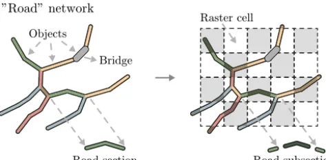
Figure 3.The road network consists of numerous objects. The ob-jects considered are bridges and road sections, which are mapped as edges in the network. Given spatial considerations during the risk assessment, the road sections are divided into subsections. The length of subsections is defined by a projected raster grid matching the grid of the hazard events.
subsections) in a way that an entity can be assigned to a sin-gle 16×16 m cell of the hazard events’ continuous fields. This is illustrated in Fig. 3.
With regards to determining the system representation, the analyzed events (organized using the generic categories in-troduced in Sect. 2) are presented next. It is worth noting that all events were described in terms of their spatial and tem-poral characteristics, and measures of the intensities were as-signed to these events to describe attributes of interest. Once these events were defined, scenarios were built considering the relationships among events as suggested by the caption of Fig. 1.
– Source event:rainfall,runoff. – Hazard events:floodsandmudflows.
– Object events:bridge local scour,road section inunda-tion,road section mud-blocking,speed reduction, and capacity reduction.
– Network events:network functionality.
– Societal events: restoration interventions, traffic changes.
To model the spatio-temporal behavior of rainfall and the changes in river discharge values, a larger area than the area used for assessing the hazard events was considered for the source events. This is illustrated in Fig. 2. The hazard and object events were bounded to the corresponding catchment area of the region. The boundaries of the network and so-cietal events exceeded the boundary of the object events to properly model the effects at the network level. The costs were only accounted for the Chur region. National-level im-pacts were not considered (e.g., blockade of the transit route from northern Europe to the south). Furthermore, scenarios were divided into time steps, with the duration of each time
step varying, depending on the occurred events in the sce-nario. Source and hazard events were observed every hour, in order to account for gradual changes of the system (e.g., the traveling paths of rainfall, the increase of river stage). Object, network, and societal events were evaluated on an hourly basis during the hazard events and on a daily basis af-ter the hazard events as the restoration time was expressed in working days.
3.3 Modules
Due to the modular approach of the simulation engine, events were represented as autonomous physical models grouped in modules, where only the metadata such as needed input and output had to be defined (a module can contain one or more models). Modules and models were developed in-house us-ing Python to support the detailed study of (i) the behavior of the comprising models as the source code was available, and (ii) the uncertainties and propagation as all variables and functions of the individual models were known and could be modified. As most network managers use geographic infor-mation systems (GIS), a GIS data interface was developed to facilitate the import and export of data. Furthermore, the program code was optimized for massively parallel comput-ing to reduce the computational time of the optimization pro-cess (i.e., each simulation ran on a designated CPU and thus an increase in the amount of CPUs increased the number of simulations for a given time frame). Brief descriptions of the modules used are provided in the following sections. For the interested reader, mathematical definitions of each module are given in the Supplement of this paper.
3.3.1 Rainfall
The experimental precipitation catalog described by Wüest et al. (2010) was used as the data source for rainfall mod-eling. The dataset covers all of Switzerland for the period between May 2003 and 2010. This catalog was derived from a combination of precipitation-gauge-based high-resolution interpolations and an hourly composite of radar measure-ments. The aggregation of the two data sources allowed for a catalog of very high resolution at the spatial scale (1 km2) and at the temporal scale (1 h). The initial precipitation fields were sampled from this catalog using randomized start hours and durations. The precipitation values for each raster cell for each time step were then scaled to associate the return period of a generated river discharge value at a location of interest with that of the rainfall (Hackl et al., 2017).
Inputs. The return period desired to be investigated6.
6The term “inputs” refers to those inputs that are provided by
Outputs. A time series of precipitation fields (i.e., raster file for every time step), where the cell values represented the rainfall intensity per time step [mm h−1]7.
3.3.2 Runoff
The modified Clark (ModClark) model by Kull and Feldman (1998) was used to estimate the runoff. After parsing a water-shed into a uniform grid (matching that of the rainfall), this model used a linear quasi-distributed transformation method to estimate the runoff based on the Clark conceptual unit hy-drograph (Clark, 1945). The method accounted for spatial differences in precipitation and losses (Paudel et al., 2009), allowing to model runoff translation and storage. The im-plementation of this model was calibrated by comparing the calculated values with measured values from the stream and precipitation gauging stations in the area.
Inputs. A time series of precipitation fields, where the cell values represented the rainfall intensity per time step [mm h−1].
Outputs. Hydrographs for different sections of the rivers in the area of study, which were generated using the excess of cells located at the basin outlets [m3s−1].
3.3.3 Flood
A one-dimensional hydraulic model for gradually varied steady flow in an open channel network was implemented for the 31 km-section of the Rhine river in the area of study. This model was used to simulate the floodplain inundation by first computing the water surface profile of a given cross-section to the next, and then interpolating inundation val-ues in between cross-sections to obtain the inundation field for the area of study. The 198 cross-sections, with an aver-age distance of 150 m between them, were obtained from a digital elevation model (DEM) of the area. The model boundary conditions were represented by (i) the discharges at Ilanz and Fürstenau, (ii) the water level at the Rhine out-let, and (iii) the evolution of the additional discharges per cross-section derived from the computed hydrographs. The (Manning) roughness coefficients were estimated based on soil cover and land use. The hydraulic model was calibrated based on historical records of the stream gauging stations in the area.
Inputs. Hydrographs for different sections of the rivers in the area of study [m3s−1].
Outputs. A time series of inundation fields (i.e., raster file for every time step), where the cell values represented the floodwater depth above ground [m].
7The term “outputs” refers to those outputs that are provided by
the module and can be used by all other modules, or ultimately can be regarded to be the estimated consequences.
3.3.4 Mudflow
The mudflow model consisted of three main processes: (i) de-termination of potential mudflow locations, (ii) modeling the potential geometries and volumes, and (iii) estimation of the probability to trigger a mudflow. Potential locations and ge-ometries were obtained from Losey and Wehrli (2013). Po-tential locations were determined using geological data and relief parameters as described in Giamboni et al. (2008), and geometries were calculated using the random walk routine of Gamma (2000). In total, 54 potential mudflows were consid-ered in the target area of study. The volume of each mudflow was then estimated by calculating the runout length of the fan using the empirical relation of Rickenmann (1999). The increase in elevation per cell was calculated by dividing the mudflow volume by the area of the fan.
The probability of occurrence was estimated by first using the empirical intensity-duration function for sub-alpine re-gions proposed by Zimmermann et al. (1997) to determine which mudflows could be triggered at a given time step. When intensity-duration thresholds were exceeded at the site of a potential mudflow, a probability of being triggered was assigned to the mudflow event. This probability was related to the corresponding estimated slope factor of safety (Skemp-ton and Delory, 1952). When determined to be triggered, the mudflow process was assumed to happen within one simula-tion time step.
Inputs. A time series of precipitation fields, where the cell values represented the rainfall intensity per time step [mm h−1].
Outputs. A time series of mudflow fields (i.e., raster file for every time step), where the cell values represented the deposited mudflow volume [m3].
3.3.5 Object fragility
The relationships between hazard and object events were rep-resented by fragility functions. These functions related haz-ard intensity measures4, such as river discharge, inundation depth, and mudflow volume, to the likelihood of meeting or exceeding a determined damage (limit) states of a bridge, road section/subsection. As fragility functions do not con-sider monetized consequences (as opposed to vulnerability functions8, which measure monetized consequence ratios), their use allows treating damages and their consequences separately. The fragility functions developed for this work were assumed to be log-normally distributed (Eq. 2), where
Sis the realization of the damage state,sis a possible dam-age state of an object,4is the observed intensity measure of the hazard event at the object location,8denotes the
stan-8Such functions are also referred to as damage functions and
dard normal cumulative distribution function, and µandσ
are the parameters of the estimated probability distribution.
P[S≥s|4] =8
ln4−µ σ
(2)
The estimated damage state exceedance probabilities out-put considered the cumulative effects of hazard events. In other words, only the maximum hazard intensity measure observed up until a time step t was used at that time step to determine the damage state exceedance probabilities. The following subsections provide specific details on the devel-opment of the fragility functions for bridge local scour, road section inundation, and road section mud-blocking.
Bridge local scour
Assuming a negligible contraction of the riverbed cross-sections (Gehl and D’Ayala, 2015), only local (pier) scour was considered for the application, resulting in the selection of five bridges that could fail as a result of this phenomenon. To quantify different levels of local scour, four damage states were defined as described in Table 1. Fragility functions were used to relate these damage states with a range of possible river discharge values for bridges with one pier and those with two piers. The method used the local scour model of Arneson et al. (2012) and a Monte Carlo scheme to gener-ate 100 000 uncertain local scour depths. These depths were compared with depth thresholds assumed to correspond to each damage state, leading to the estimation of damage state exceedance probabilities. The derived fragility parameters are given in Table 2. The fragility functions are illustrated in Fig. 4.
Road section inundation
The determination of the probable damages of a road sec-tion, whether part of a major or minor road, due to floods is an active field of research. The small amount of available data makes describing such relationship in a numerical form a challenging task. Some works (e.g., De Bruijin, 2005; Kok et al., 2005; Koks et al., 2012; Tariq et al., 2014; Li et al., 2016) have sought to numerically describe the relationship between damages and inundation depth. However, there are observed differences in the methods and results (e.g., some works bundled direct and indirect costs in their estimates), leading to the conclusion that these numerical relationships can only be applied to specific contexts and confined geo-graphical areas.
To overcome this challenge, a different approach was taken, which involved proposing fragility functions based on data and information published by previous works seeking to qualitatively illustrate the impact of floods on road sections (e.g., ALA, 2005; ADEPT, 2011; Walsh, 2011; Vennapusa et al., 2013; Roslan et al., 2015). Despite the use of these
studies, the proposed functions remain to be coarse illustra-tions that cannot be used in practice without further analy-sis. To qualify different levels of damage, four damage states were defined as described in Table 1. The fragility function parameters are given in Table 2. The fragility functions are displayed in Fig. 4.
Road section mud-blocking
To determine the level of road section mud-blocking, a dis-tinction was made between high-speed (major) and local (mi-nor) roads. The damage states defined by this work were based on the descriptions of Winter et al. (2013). These states are shown in Table 1. Fragility functions were estimated us-ing expert data from the survey conducted by Winter et al. (2013), where experts were asked to relate debris flow vol-umes and damage state exceedance probabilities for differ-ent damage states and road categories (in doing so, it was here assumed that the results of this survey, focused on debris flow, could be used for determining a relationship between mudflows and road sections). The fragility function parame-ters are given in Table 2. The fragility functions are shown in Fig. 4.
Inputs. (i) Hydrographs for different sections of the rivers in the area of study (out of which only those hydrographs for the river sections with the bridges of interest were selected during the analysis) [m3s−1], (ii) a time series of inundation fields, where the cell values represented the floodwater depth above ground [m], and (iii) a time series of mudflow fields, where the cell values repre-sented the deposited mudflow volume [m3].
Outputs. Time series of damage state exceedance probabil-ities considering cumulative damages for bridges due to local scour, road sections/subsections due to inundation, and road sections/subsections due to mud-blocking. 3.3.6 Object functionality
In terms of loss of functionality, a distinction was made be-tween speed reduction and capacity reduction. The reduc-tion of travel speed was used as a temporary measure during the hazard events period, indicating the drivers’ response to the changed driving conditions (i.e., on an inundated road, drivers reduced their speed). In addition to this temporary measure, it was assumed that damages in objects would re-sult in reduction of capacity (lane closure). In order to return to an adequate level of service, such objects had to be re-paired (see Sect. 3.3.10).
Speed reduction
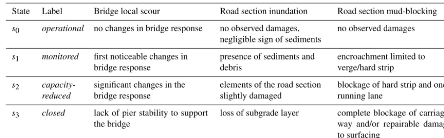
Table 1.Damage states for bridge local scour, road section inundation and road section mud-blocking.
State Label Bridge local scour Road section inundation Road section mud-blocking
s0 operational no changes in bridge response no observed damages, negligible sign of sediments
no observed damages
s1 monitored first noticeable changes in bridge response
presence of sediments and debris
encroachment limited to verge/hard strip
s2
capacity-reduced
significant changes in the bridge response
elements of the road section slightly damaged
blockage of hard strip and one running lane
s3 closed lack of pier stability to support
the bridge
loss of subgrade layer complete blockage of
carriage-way and/or repairable damage to surfacing
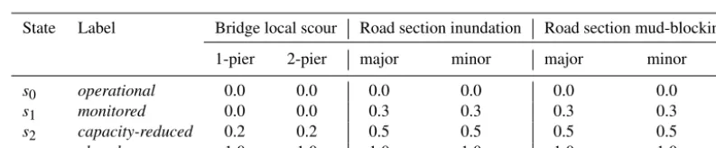
Table 2.Fragility function parameters for bridge local scour, road section inundation and road section mud-blocking.
State Label Bridge local scour Road section inundation Road section mud-blocking
1-pier bridge 2-pier bridge major road minor road major road minor road
µ σ µ σ µ σ µ σ µ σ µ σ
s0 operational – – – – – – – – – – – –
s1 monitored 5.52 0.66 4.67 0.64 2.71 0.74 1.61 0.92 9.07 3.45 7.70 3.70
s2 capacity-reduced 8.34 0.58 7.44 0.54 3.00 0.87 2.30 0.93 10.6 2.92 9.28 3.31
s3 closed 10.1 0.61 9.10 0.54 3.22 1.00 2.71 1.00 11.5 2.28 9.79 2.51
An exponential function was fitted to these data to describe the limit vehicle speed in a road as a function of inundation depth. The maximum acceptable velocity that ensures safe control of a vehicle through a specific section at a certain time when considering the inundation depthiwas estimated byv=vmax·e−0.10814·i. Wherevmaxdescribes the maximum allowed speed on a road (e.g., 120 km h−1). It was assumed that vehicles were only operated until an inundation depth of 0.3 m.
Capacity reduction
The relationships between the hazard events and the reduc-tion in capacity were represented by funcreduc-tional loss funcreduc-tions (Lam and Adey, 2016). Expected functional losses were de-termined as functions of time-dependent hazard intensities
4, damage statesprobabilities derived from fragility func-tions’ damage state exceedance probabilities, and functional loss valuesλassociated with the investigated damage states (Eq. 3). The expected functional loss of a specific object at a specific time in the simulation is represented byhλi ∈ [0,1].
hλi =E(λ|4)=X
s
E(λ|s)·P[S=s|4] (3)
Table 3 presents the estimated loss values λ used. The values were either directly obtained or inferred from a sur-vey conducted by D’Ayala and Gehl (2015). A loss value of
λ=0 represents no reduction in capacity (i.e., all lanes are open) while a loss value ofλ=1 indicates that no capac-ity is available (i.e., all lanes are closed). The functional loss functions are illustrated in Fig. 5.
Inputs. (i) A time series of inundation fields, where the cell values represented the floodwater depth above ground [m], and (ii) time series of damage state ex-ceedance probabilities considering cumulative damages for bridges due to local scour, road sections/subsections due to inundation, and road sections/subsections due to mud-blocking.
Outputs. (i) A time series of speed reduction for inun-dated road sections/subsections, and (ii) time series of expected capacity reduction for bridges with scoured piers, inundated road sections/subsections and mud-blocked road sections/subsections.
3.3.7 Object restoration needs
101 102 103 104 105 0.0
0.2 0.4 0.6 0.8 1.0
River discharge [m3 s ]
Damage
state
exceedance
pro
babili
ty
Bridge local scour
1-pier
s1
s2
s3 2-pier
s1
s2
s3 (a)
100 101 102 103 104 105 0.0
0.2 0.4 0.6 0.8 1.0
Mudflow volume [m3]
Road section mud-blocking
s1
s2
s3 (c)
0.0 0.05 0.10 0.15 0.20 0.25 0.30 0.0
0.2 0.4 0.6 0.8 1.0
Inundation depth [m] Road section inundation
s1
s2
s3 (b)
-1
Minor Major
Minor Major
Figure 4.Fragility functions for(a)bridge local scour,(b)road section inundation, and(c)road section mud-blocking. The horizontal axis represents the intensity measure4of the corresponding hazard. For(a)bridge local scour and(c)road section mud-blocking the axes are displayed in log-scale. The vertical axis represents the exceedance probabilities for the different damage states. The parametersµandσ of these functions are given in Table 2.
Table 3.Functional loss estimations for bridge local scour, road section inundation, and road section mud-blocking.
State Label Bridge local scour Road section inundation Road section mud-blocking
1-pier 2-pier major minor major minor
s0 operational 0.0 0.0 0.0 0.0 0.0 0.0
s1 monitored 0.0 0.0 0.3 0.3 0.3 0.3
s2 capacity-reduced 0.2 0.2 0.5 0.5 0.5 0.5
s3 closed 1.0 1.0 1.0 1.0 1.0 1.0
is replaced by the functional loss during the restoration inter-vention (in this application, these losses were assumed to be the same as those in Table 3), restoration times and restora-tion costs.
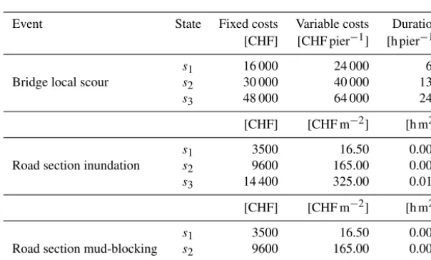
While a restoration cost was composed of a fixed part (e.g., site setup) and a variable part (e.g., CHF m−2of pavement, CHF m−3of concrete, where mu stands for monetary units), the corresponding restoration time was approximated as a single value (i.e., no distinction between activities related to fixed and variable costs). These costs and durations are shown in Table 4. Cost estimates were based on Staubli and Hirt (2005) and from a survey conducted by D’Ayala and Gehl (2015). For each damage state, a restoration strategy was derived, and for each strategy, a restoration cost9and a restoration time were approximated. It was assumed that the selected restoration program did not affect intervention costs.
Inputs: Time series of damage state exceedance probabili-ties considering cumulative damages for bridges due to local scour, road sections/subsections due to inundation, and road sections/subsections due to mud-blocking. 9Costs taken from the literature were adjusted to 2017 price
lev-els. To avoid over interpreting the specific values that were in the application, monetary units are used instead of real currency.
Outputs: Time series of the expected capacity reduction during restoration intervention, restoration costs [CHF], and restoration times [h] for bridges with scoured piers, inundated road sections/subsections and mud-blocked road sections/subsections.
3.3.8 Network
101 102 103 104 105 0.0
0.2 0.4 0.6 0.8 1.0
Exp
ected
capacit
y
reduction
h
λ
i
Bridge local scour
1-pier 2-pier (a)
0.0 0.05 0.10 0.15 0.20 0.25 0.30 0.0
0.2 0.4 0.6 0.8 1.0
Inundation depth [m] Road section inundation (b)
100 101 102 103 104 105 0.0
0.2 0.4 0.6 0.8 1.0
Mudflow volume [m3]
Road section mud-blocking (c)
River discharge [m3 s-1]
Minor Major Minor Major
Figure 5.Functional loss functions for(a)bridge local scour,(b)road section inundation, and(c)road section mud-blocking. The horizontal axis represents the intensity measure4of the corresponding hazard. For(a)bridge local scour and(c)road section mud-blocking the axes are displayed in log-scale. The vertical axis represents the expected functional loss.
Table 4.Restoration costs and times for bridge local scour, road section inundation, and road section mud-blocking.
Event State Fixed costs Variable costs Duration
[CHF] [CHF pier−1] [h pier−1]
s1 16 000 24 000 60
Bridge local scour s2 30 000 40 000 135
s3 48 000 64 000 240
[CHF] [CHF m−2] [h m2]
s1 3500 16.50 0.005
Road section inundation s2 9600 165.00 0.009
s3 14 400 325.00 0.015
[CHF] [CHF m−2] [h m2]
s1 3500 16.50 0.005
Road section mud-blocking s2 9600 165.00 0.009
s3 14 400 325.00 0.015
Once aggregated to the section level, functional losses, restoration costs, and restoration times for road sections, along with those for bridges, were assigned as attributes to the network. This required modeling the road network as a graph composed of 1520 vertices (i.e., 37 centroids, 1056 junctions, and 427 changes in road geometric features) and 3202 directed edges, where each edge represented a bridge or a road section. As the road network is located in a moun-tainous area, the topology of the network is such that certain areas are served by a single road, which means that, if part of this road is disrupted, there is no valid rerouting alterna-tive and part of the demand remains unsatisfied. This results in missed trips. For this network, in particular, these edges (also referred to as cut links) represented about 11 % of the entire edge set.
After the hazard events period, the network was restored using a restoration model. This model supported the
updat-ing of damaged objects to restored objects (see Sect. 3.3.10), leading to updated network graphs to be used in the traffic model to estimate the indirect costs.
Inputs. (i) A time series of speed reduction for inundated road sections/subsections; (ii) time series of expected capacity reduction for bridges with scoured piers, inun-dated road sections/subsections, and mud-blocked road sections/subsections; (iii) time series of the expected ca-pacity reduction during restoration intervention, restora-tion costs [CHF], and restorarestora-tion times [h] for bridges with scoured piers, inundated road sections/subsections, and mud-blocked road sections/subsections; and (iv) a restoration program, defining when each damaged ob-ject is to be restored.
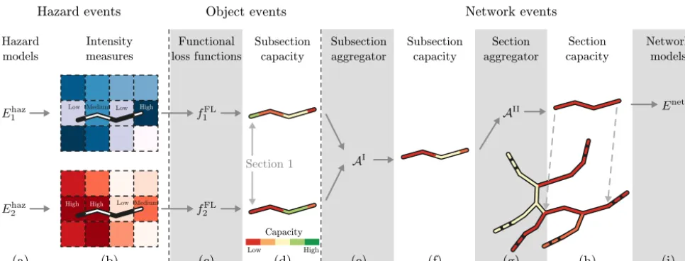
Low Medium High Low
Capacity
Hazard
models
Intensity
measures
Functional
loss functions
Subsection
capacity
Subsection
capacity
Hazard events Object events
Section 1
Subsection
aggregator
Section
aggregator
Section
capacity
Network events
Network
models
(a) (b) (c) (d) (e) (f) (g) (h) (i)
Low High High High
Medium Low
Figure 6.The hazard events(a)were represented in the form of a spatially distributed grid where the intensity measures change for each cell(b). Each road section of the network had to be split up according to this grid, which resulted in a set of subsections. This process was also previously illustrated in Fig. 3. In this specific example, the considered section is split into four subsections(b). The intensities are then processed independently for each of these subsections. For each intensity measure, the expected functional loss (i.e., speed reduction, capacity reduction) for each subsection is determined using computed functional loss functionsf1FLandf2FL(c). Schematized in panel(d) are the resulting functional losses that are encoded in the colors of the subsections. A subsection aggregatorAI(e)is executed for each subsection and combines all functional loss values derived from different hazard events into a single value(f). This aggregator simply takes the maximum functional loss values. Finally, a section aggregatorAII(g)combines the functional losses of the subsections into a single functional loss for the section(h). Losses at the section level are then used in the network model(i). (This figure was adapted from Heitzler et al., 2018.)
the expected capacity reduction during restoration inter-vention, restoration costs [CHF], and restoration times [h] for bridges with scoured piers, inundated road sec-tions, and mud-blocked road sections.
3.3.9 Traffic
Vehicle travelers were assumed to behave according to the user equilibrium principle, which states that they choose a route from their origin to their destination that minimizes their travel cost. This means that the travel cost between each origin–destination pair is uniquely defined (Jenelius et al., 2006). This cost depends on the travel costs of all edges in an origin–destination path, which change with traffic flow. A stable state is reached only when no traveler can reduce his/her own costs of travel by unilaterally changing routes (Sheffi, 1985). Travel time was estimated using the formula-tion proposed by the Bureau of Public Roads (1964).
Regarding the demand model, the origin–destination ma-trix was estimated by a gravity model based on population density and was related to the number of vehicles on an av-erage hourly and an avav-erage daily basis. This matrix was calibrated and updated using information of recent traffic counts along a set of edges. The study area was divided into 37 zones. Every internal centroid corresponded on average to an area of 15 km2with a population of about 1000.
To reduce computational complexity, only changes in route choices were considered within the risk assessment
(i.e., travel demand was assumed to be inelastic). This was deemed a reasonable assumption as a large majority of the travel demand was caused by trips to work, which are made under normal circumstances. Therefore, changes in destina-tion choices, mode choices, or trip frequencies were not con-sidered. Moreover, it was assumed that the duration of net-work closures was long enough for all travelers to be aware of them so that a new user equilibrium could be reached. Inputs. A time series of routable network graphs that can be
used for traffic assignment.
Outputs. (i) A time series of traffic flow and travel time for each edge in the network, (ii) a time series of missed trips in the network, and (iii) a time series of damaged bridges and road sections that caused loss of connectiv-ity.
3.3.10 Restoration
10 reconstruction crews could work simultaneously and each crew could at most be assigned to one object. For each day until the restoration was finished, the model updated the ob-jects’ states and executed the traffic model described to sup-port the estimation of indirect costs during the restoration period. The restoration process ended once the network was completely restored.
Inputs. (i) Time series of the expected capacity reduction during restoration intervention and restoration times [h] for bridges with scoured piers, inundated road sections, and mud-blocked road sections; and (ii) a time series of damaged bridges and road sections that caused loss of connectivity.
Outputs. A restoration program, defining when each dam-aged object is to be restored.
3.3.11 Direct and indirect costs
The direct costs were estimated to be the sum of the di-rect costs for each intervention to be executed during the restoration period. These costs were actually accrued dur-ing the hazard events period as bridges and road sections were impacted by the hazard events (see Sect. 3.3.7). The direct costs were composed of a fixed part (e.g., side setup) and a variable path (e.g., CHF m−3of pavement). The direct costs associated with each damage state are given in Table 4. The indirect costs were comprised of costs for the prolon-gation of travel time and costs due to a loss of connectivity. These costs were accrued during the hazard events period and the restoration period. The travel time costs were estimated based on the increased amount of time vehicles spent trav-eling. The Swiss Association of Road and Transport Experts (VSS, 2009a) approximated the travel time cost per vehicle to be 23.29 CHF h−1. In addition to considering the time factor, indirect costs also accounted for the costs of vehicle opera-tion, which were incurred as a result of fuel consumption and vehicle maintenance. Based on the estimates of VSS (2009b), the mean fuel price was approximated with 1.88 CHF L−1 with a mean fuel consumption of 6.7 L/100·veh km and the operating costs per vehicle without fuel consumption was as-sumed to be 14.39 CHF/100·veh km. The costs due to a loss of connectivity were estimated based on the unsatisfied de-mand and the resulting costs due to missed trips. For every hour of delay of a trip, costs in the amount of 83.27 CHF were charged.
Inputs. (i) A time series of the expected restoration costs [CHF] for bridges with scoured piers, inundated road sections, and mud-blocked road sections; (ii) a time se-ries of traffic flow and travel time for each edge in the network; and (iii) a time series of missed trips in the network.
Outputs. Time series of the estimated direct and indirect costs.
4 Results
The results section is organized in three subsections that present (i) the results of a single simulation run, (ii) the ag-gregation of results of multiple simulations with the same return period, and (iii) the results of multiple scenarios with multiple return periods.
4.1 Single scenario
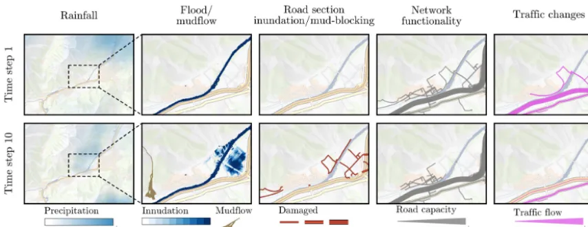
Figure 7 shows the changes in a scenario due to a flood of 500 year return period. For this specific chain of events, the hazard events extended over a period of 18 h while the restoration period lasted 23 days (please note that while only two time steps are shown in this figure, the full system evo-lution is given in the Supplement).
In this scenario, the rainfall started at hour 1 and ended at hour 10, with the maximum precipitation observed around hours 6 and 7. The precipitation moved from the northwest-ern part of the study area to southeastnorthwest-ern part. At hour 6, parts of the motorway to Fürstenau were flooded, which led to a detour of the traffic through the village of Bonaduz. At hour 8, the motorway was flooded between Tamins and Do-mat/Ems, which interrupted the west–east connection in the valley. Traffic had to detour through Chur and drive south. Due to the lag runoff, the maximum extent of the flood was reached at hour 11. Most of the flood damage was caused in the western part of Chur, while in the northern part, only the motorway and several minor roads were flooded. Addition-ally, the triggering of a mudflow next to the village of Fels-berg can be observed in hour 10, causing the blockage of two minor roads. This type of analysis is useful, to investigate the spatial and temporal evolution of the events. However, a sin-gle scenario cannot capture the uncertainties of the events. To overcome this issue, multiple scenarios with the same initial conditions (i.e., the same return period) can be performed.
Figure 7.Spatio-temporal representation of the system. The columns represent the investigated events, while the rows illustrate different time steps of the considered scenario. Time step 1 represents the beginning of the simulation with all elements at their initial state. Time step 10 illustrates the system state close to the peak of the flood. As observed, road sections were damaged by the flood, which resulted in functional losses and a change of traffic flow. In this scenario, people living in the northern part of the area were cut off from the rest of the network due to severely inundated roads.
whole system, and hence no clear spatial positions can be assigned to them.
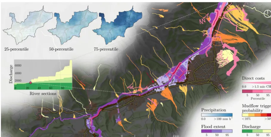
As illustrated in Fig. 8, the mapped floods can be inter-preted as a probabilistic hazard map for events of a 500 year return period. While such maps can be used to reach some conclusions about the probable inundated areas, it is possible to also use geostatistical tools to analyze these and other in-formation. Figure 9 shows the automatic cluster of damaged objects in the network using a mathematical algorithm that also supports the visualization of the associated direct costs. Such analysis can also be used for the planning of mitigation measures as part of the management of risk.
Figure 9 gives additional insights on the resulting costs. Direct costs followed a heavy-tailed distribution (i.e., scat-tered high values in the positive direction of the distribu-tion). Such distributions are often observed when consider-ing extreme events, which is the case in the application that modeled random mudflows in addition to floods. For exam-ple, a mudflow was occasionally triggered in cluster five (see Figs. 8 and 9). When the mudflow was not triggered, little to no damage was observed in this cluster; however, when the mudflow was triggered, severe damage occurred. Contrary to direct costs, indirect costs followed a symmetric distribu-tion due to the network redundancy (i.e., as long the network is not completely out of service, vehicles can take detours, leading to a redistributing of the indirect costs).
4.3 Multiple scenarios with multiple return periods Figure 10 shows the obtained risk curves (return period vs. costs) with confidence intervals and annualized risk esti-mates (how much risk can be expected per year on average over a long period of time). Once a risk curve of a specific percentile was determined, its corresponding costs were used
to estimate the matching annualized risk using Eq. (4) (Deck-ers et al., 2009), whereRais the annualized risk andC
i the
costs associated with the annual exceedance probability T1
i,
which is estimated based on the return periodT of the event
i. To use this equation, the events had to be arranged in de-creasing order (e.g.,12,15, . . . ,10 0001 ).
Ra=X
i
1
Ti
·(Ci−Ci−1) (4)
When using this equation, direct costs were found to fol-low a heavy-tailed distribution. The median annualized risk related to direct consequences (CHF 1.5 million) was larger than that of indirect consequences (CHF 1 million). If other indirect consequences had been considered in addition to prolongation of travel time and missed trips (e.g., business interruptions), the annualized risk related to indirect conse-quences would be expected to increase significantly.
5 Discussion
Figure 8.Aggregation of multiple simulations for hazard events with 500 year return period. This map visualizes the uncertainties related to these events. For example, only 5 % of the floods exceeded the light purple floodplain (95 % percentile), while only 5 % of the floods resulted in floodplains smaller than the dark purple area (5 % percentile).
(a) Heatmap of direct costs
1 2 3 4 5
0 1 2 3 4 5 10 15 20 25
Clusters of impaired sections
Costs
[CHF
·
10
6]
Direct costs per cluster (b)
Direct Indirect 5
10 15 20 25 30 35 40 45 50
Consequences
Costs
[CHF
·
10
6]
Costs (c)
Figure 9.Direct and indirect costs related to the hazard events with 500 year return period. A heat map of expected direct costs for all sce-narios(a)can be used to analyze high-risk areas. Here, five clusters were detected. The estimated direct costs per cluster and their associated uncertainties are illustrated in panel(b)using box plots. While in the second cluster, the median direct cost was around CHF 4.8 million, in the fifth cluster, a much smaller median value was estimated. However, the uncertainty of this cluster on the positive direction was compara-ble to that of the second cluster in the same direction. Comparing direct and indirect costs(c), their medians were similar. Nonetheless, the distribution of direct costs was positively skewed (heavy tail) while the distribution of indirect costs was close to symmetrical.
had full knowledge of the traffic conditions). Moreover, the traffic model did not account for dynamic phenomena like queues, spillbacks, wave propagation, or changes in travel patterns after a disruptive event (although studies show these can be considerably different after a disruptive event; e.g., Chang and Nojima, 2001; Kontou et al., 2017). In general, the integration of more sophisticated models can potentially lead to improved risk estimates. A prerequisite for this in-tegration is conducting uncertainty and sensitivity analyses
to prioritize the parts of the system to be analyzed in more detail.
Figure 10.Risk curves and annualized risk estimations. The risk curves related to direct and indirect costs are illustrated in(a). The 50 % and 90 % confidence intervals are given for the sum of the costs. Costs associated with individual simulation runs are illustrated as gray dots. Equation (4) was used to calculate the annualized risk(b)for different cost percentiles. The median annualized risk for the sum of the costs was found to be CHF 2.4 million.
of the simulation engine may be applied independently (e.g., to investigate the probability of bridge failure due to local scour at a given location). Hence, the system may be prof-itably used for a number of additional purposes (e.g., as a tool for cost-benefit analysis of flood and mudflow protec-tion measures, as a decision support system for operaprotec-tional flood and mudflow control). As implemented, the risk assess-ment can provide a mechanism for a region-wide screening of priority locations for risk reduction based on the analysis of the road network and traffic properties (e.g., Heitzler et al., 2017). This function can be enhanced with the use of visu-alization tools, enabling network managers to dynamically see how different environmental systems (i.e., rainfall, flood and mudflow) influence each other, and how their impact on networks can affect society (Heitzler et al., 2016).
Finally, combining several models results in a significant degree of uncertainty. Whenever possible, the results should be compared with and calibrated against empirical data, when available. For example, the probability of damages ob-tained through simulations could be calibrated against col-lected data from field structural surveys when such data ex-ist. Calibration for societal events is rather difficult because such data are difficult to measure and monitor. Nonetheless, in some cases, basic data are available, including the duration of a network’s loss of functionality and the estimated number of network users affected.
6 Conclusions
The purpose of estimating the risk related to networks is, among others, to provide an overview of the probable adverse events that may negatively affect the network, assess their so-cietal effects (e.g., costs), and provide a basis for planning risk-reducing interventions. Assessing the risk related to
net-works exposed to multiple types of hazards is not trivial due to the large number of events that need to be modeled in an integrated manner, their uncertainties and the propagation of these uncertainties affecting risk estimates. This is particu-larly evident when dealing with complex system representa-tions, where the costs of indirect consequences can be multi-ple times higher than the costs of direct consequences, with no linear relationship between these types of cost.
This paper describes a risk assessment methodology for networks when there is a need to represent the system con-taining these networks using various degrees of complexity. The methodology is supported by a modular simulation en-gine that fosters multidisciplinary collaboration. Following this methodology, a state of the art application was designed and implemented, which aimed at estimating the spatio-temporal risk of a road network in Switzerland due to the occurrence of a time-varying rainfall that caused flood and mudflow events. To achieve this objective, the modular simu-lation engine was used to couple rainfall, runoff, flood, mud-flow, damages, functional losses, traffic, and restoration mod-eling. Consequences were monetized into direct and indirect costs, considering restoration interventions, prolongation of travel time, and missed trips. The costs of the 1200 scenarios simulated were analyzed at three different levels: (i) those of a single simulation, (ii) those of multiple simulations with the same return period, and (iii) those of multiple simulations of multiple return periods. This number of scenarios supported the analysis of cost uncertainties.