c
Owned by the authors, published by EDP Sciences, 2015
Using plastic instability to validate and test the strength law of a material
under pressure
Cyril Bolisa, Denis Counilh, and Brice Savale CEA, DAM, DIF, 91297 Arpajon, France
Abstract. In dynamical experiments (pressures higher than 10 GPa, strain rate around 104–106 s−1), metals are classically
described using an equation of state and a strength law which is usually set using data from compression or traction tests at low pressure (few MPa) and low strain rates (less than 103 s−1). In consequence, it needs to be extrapolated during dynamical
experiments. Classical shock experiments do not allow a fine validation of the stress law due to the interaction with the equation of state. To achieve this aim, we propose to use a dedicated experiment. We started from the works of Barnes et al. (1974 and 1980) where plastic instabilities initiated by a sinusoidal perturbation at the surface of the metal develop with the pressure. We adapted this principle to a new shape of initial perturbation and realized several experiments. We will present the setup and its use on a simple material: gold. We will detail how the interpretation of the experiments, coupled with previous characterization experiments helps us to test the strength lax of this material at high pressure and high strain rate.
1. Introduction
Testing and validating strength law at high pressure and high strain rate is a challenging problem. Classically, these laws are set using characterization experiments such as Hopkinson’s bars or compression/traction machines at low pressure and low strain rates (lower than 103s−1). Even with these limitations, they are used to simulate shock experiments where the pressure is driven by explosives or by laser shots and where the strain rate can reach 104 to 107s−1. Without any direct data at these regimes, the material behavior has to be extrapolated.
To validate this extrapolation, we looked at experi-ments which are directly sensitive to the strength law. Usual shock experiments are often dedicated to equation of state measurements and are only sensitive to the strength law in a second order. To have direct measurements, we were inspired by the works of Barnes et al. [1,2] who made the link between the growth of Rayleigh-Taylor instability and the strength law. Since the last years, this technic was upgraded using laser driven plasmas to generate pressures over 1 Mbar [3] of proton radiography at Prad [4] to achieve multiple views of the perturbation growth.
In this paper, we will show how we were inspired from Prad experiments to design our Rayleigh-Taylor instability experiment. We will present the principle and the setup that was tested with two gold targets. The results of the two experiments are analyzed and compared to numerical simulations. Lastly, we will discuss how to fit the perturbation growth by changing the parameters of the strength law.
aCorresponding author:cyril.bolis@cea.fr
h
Target PWG
X-ra
y
ge
n
era
tor Films
Figure 1. Principle of the experiment.
2. Experimental setup
2.1. Principle
Similarly to the technic developed by Barnes, we used a high explosive plane wave generator (PWG) to generate the pressure (Fig. 1). The target is located a few millimeters from the surface of the explosive (HMW based). Therefor, the pressure is generated by the release of detonation products. It can be assimilated to an isentropic compression which produces the growth of an axisymmetric perturbation at the center of the target in front of the plane wave generator.
During the experiment, the shape of the target is acquired using low energy X-ray generator (mean spectra 80 keV) coupled to radiographic films on which we measure the position of the target and the perturbation length (h in Fig. 1). As the perturbation is axisym-metric, three couples generator/film on different axis
-1 0
1 2
3
-12 -9 -6 -3 0 3 6 9 12
X (
m
m
)
Y (mm)
T1 T2
Figure 2. Targets shapes.
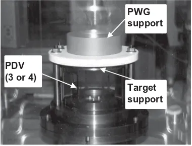
Figure 3. Target support: upper view.
PDV (3 or 4)
PWG support
Target support
Figure 4. Target support: side view.
(around every 120◦) are used to image the target at three different times.
To test our setup, two experiments were realized (T1 and T2) using two different target shapes (Fig. 2). Main differences arise from the target thickness and the perturbation shapes (Gaussian for T1, design by simulation for T2) and amplitude (900µm for T1, 300µm for T2). For both targets, pure gold was chosen as a well-known and simple material.
2.2. Setup
The setup of the experiment is presented on the next figures. The target is supported by two metallic pieces, in light metal (aluminum for T1 and copper for T2) and in heavy metal (tungsten in both cases) (Fig.4). The first one will flight faster than the target whereas the second one will
Figure 5. Pyrotechnic protections and radiographic chain.
almost not move. This setup allows us to avoid some side effects and to ensure the visibility of the target during the experiment.
The plane wave generator is mounted in front of the perturbation at a fixed distance (Fig. 4) at the opposite side, under the radiographic windows, three (four for T2) PDV probes are used to follow the first moment of the acceleration of the target.
The setup is placed inside a closed glass cylinder which is used to make primary void around the target. It is also used as a first pyrotechnic protection for the three radiographic chains. The second one is assured by a steel cylinder with steel plates in the radiographic axes. The holes in the cylinder are used as collimators for the X-rays. In front of each source, a box containing sensitive films is placed (Fig.5).
For each experiment, all data were acquired. The target flight is recorded on the films and the perturbation length is measured (Fig. 6). Its evolution is clearly visible on radiography at the three times. One can noticed on the bottom of the image at 20.4µs the trace of support in copper, whereas the one in tungsten stay at the top of the image.
3. Results and first simulations
Before discussing of the perturbation growth, the pressure law applied to the target has to be checked first. For this, the velocities signals for the first moments and the target position for the later ones were used.
Simulations were realized using a hydrocode in an eulerian scheme. Plane wave generator was simulated using a JWL equation of state and an Arrhenius’s type kinetic of detonation. The mesh size was 50µm square.
3.1. Velocities
Three PDV probes were used to measure the beginning of the acceleration of the target at r=7 mm (on T2 a fourth PDV probe was used to follow the center of the target but did not give relevant results). These probes record only a few microseconds of the flight due to the detonation products which shadow the target.
Figure 6. Radiographies from the second experiment.
can be noticed that velocities on T2 were recorded on a longer duration. This can be explained by the differences on the choice of the light support (aluminum for T1, copper for T2). The copper piece is heavier and moves slower than the aluminum one. In T2, the detonation products had to wait longer before the support let them leak in direction of PDVs. This allows us to check that the second acceleration of the target (around 12µs) is also well reproduced.
3.2. Targets position
For longer times, we focused on the position of the target (r=10 mm in front of PWG) at radiographic times. This position was measured on films and on simulations using the same technique. The comparison between experiments and numerical simulations is presented in Fig.8and shows a very good agreement for the two shots.
Having the first part of the acceleration with PDVs and the later part with the position of the target, we can conclude that the simulation well describes the pressure law generated by the plane wave generator and applied to the target during the experiment. The simulation of the growth of the perturbation can now be discussed in detail.
0 200 400 600 800
10.5 11 11.5 12 12.5
Veloc
ity (m.s
-1)
Time (µs)
Exp.
Sim.
T1
0 200 400 600 800 1000 1200
10 11 12 13
Ve
lo
ci
ty (
m
.s
-1)
Time (µs)
Exp. Sim. T2
Figure 7. Velocities at r=7 mm: Comparison between experiments and simulations.
7 9 11 13 15 17 19 21
20 22 24 26
T
arget p
os
ition
(m
m)
Time (µs) Sim.
Exp.
T1 T2
Figure 8. Target position: comparison between experiments and
simulations.
4. Perturbation length
4.1. Strength law
The method used to adjust the parameters of the strength law of gold on the two experiments is discussed here. The material used for the targets was previously characterized and a Steinberg Cochran Guinan’s law (SCG [5]) was set. The formulation of the law is reminded in formulas (1) for the shear modulus (G) and (2) for the elastic limit (Y). As gold is a fcc metal, its dependency to strain rate should be weak and the SCG model should be sufficient for a first approach.
G=G0
1+ G
P
G0 P
ρ ρ0
−1 3
+ GT
G0
(T−T0)
3.5 4 4.5 5 5.5 6 6.5 7
20 22 24 26
Perturbation le
ngth
(mm)
Time (µs)
Ref G0 -70% Gpp +200% Ymax +120% Exp
T1
4 4.5 5 5.5 6 6.5 7 7.5 8
20 22 24 26 28
Perturabati
on length
(mm)
Time (µs)
Ref G0 -80% Gpp +290% Exp
T2
Figure 9. Perturbation length for the two shots and comparison
between fitted simulations.
Y = G(P,T ) G0
minY0(1+β εP)n; Ymax
. (2)
Various simulations have been led to test the growth rate sensibility to the different part of the material description (equation of state, damage, mesh . . . ). Only the strength law exhibits a real effect on the growth rate.
4.2. Uncoupled simulations
In this part, the parameters of the strength law were adjusted separately for the two experiments. The initial shear modulus (G0), its pressure derivative (GP=Gpp in figures) and the maximal elastic limit (Ymax) were fitted separately for the two shots. Results are shown in Fig.9. In both cases, the simulations using the reference parameters (ref in the following figures) overestimate the perturbation length. By modifying the parameters, simulations can be adjusted at the three experimental times. But, the changes of the parameters are not consistent between the two experiments. Thus, the pressure derivative of the shear modulus has to be increased at+200% for T1 and+290% for T2 whereas no adjustment can be achieve using Ymax for T2. Other tests have been carried out with other sensitive parameters without more success.
One can notice that the behavior is opposite between the initial shear modulus (G0−70% for T1) and its pressure derivative (GP+200% for T1) whereas they both seem to play in the same way in formulas. In fact, the difference comes from one hypothesis of the SCG model where the pressure derivatives of the shear modulus and
Figure 10. Perturbation length: Distance from simulations to
both experiments (dash line=minimum error line).
of the elastic limit are equal (term G(P,T)/G0 in Eq. (2)). If the two derivatives (GPand YP) are separated, it can be observed on simulations that the dependency raises from the pressure derivative of the elastic limit (YP) which has to be increased by+200% for T1.
This first test evidences that the growth rate of the two experiments using different initial perturbation shapes cannot be adjusted using only one parameter. A coupled research using more parameters will be discussed in the next paragraph.
4.3. Coupled simulations
In this part, the two experiments were adjusted simultane-ously using more than one parameter at a time. Due to the number of parameters to test and the time required by each simulation, a Monte-Carlo’s like approach where several sets of parameters are computed using a random law was used. For each set, the simulations for the two shots were computed and the distance between the experimental perturbation lengths and the numerical ones was measured. The first run of simulations did not show any consistency until a dependency of several parameters was exhibit. Thus, Fig. 10 shows the distance between simulations and experiments as a function of the hardening parameter n and the product GPYmax. In this graph, the existence of a valley of minimum error (symbolized by a dash line) which emphasis a correlation between these parameters can be observed.
This correlation between n and Ymaxin the SCG model can be understood using an energetic approach. Indeed, for a given experiment (energy given by the pressure law ≈ mechanical energy) and a given perturbation growth (≈ strain), different sets of parameters can achieve the same final mechanical energy (Fig.11).
0 0.1 0.2 0.3 0.4 0.5 0.6 0.7 0.8
0 0.5 1
Str
es
s (G
Pa)
Ymax = 0.31 GPa, n= 0.7 Ymax = 0.50 GPa, n = 0.5
Figure 11. Stress/strain curves for two sets of parameters having
the same mechanical energy at strain=1.
Figure 12. Iso-mechanical energy for a given strain as a function
of n and Ymax.
as observed in Fig. 10 is found. The two experiments having the same characteristics (same explosives, same distance), the pressure is similar on both experiments and the influence of GPis the same.
From the research of parameters, the five best sets can be extracted. They all show various values (1st set: GP=4.98, n=0.35, Ymax=295 MPa, 5thset: GP=3.97, n=0.41, Ymax=264 MPa) but with an error to exper-iment lower than the experexper-imental uncertainty. Target shapes at latest time are well reproduced as shown in Fig.13.
Using several parameter modifications, we succeeded to simulate the two experiments with the same strength law. From this study, we have also shown that these sets are probably not unique and that other solutions can be achieved.
4.4. Comparison to characterization experiments
To try to reduce the possibilities, the best sets were compared to characterization experiments. None of them allow reproducing the behavior identified in the past and well fitted by the reference set (Fig.14). At the opposite, the new parameters almost fit data from Suzuki et al. [6].
In their article, Suzuki et al emphasizes the sensitivity of pure gold to its microstructure and the way samples are prepared. A first hypothesis to explain the difference with previous characterization can be an effect of the machining
-3 -2 -1 0 1 2 3
7 12 17
y (m
m)
x (mm) Exp
Ref set
1st set
5th set
T1 - 26 µs
8 13 18
x (mm) T2 - 26.4 µs
Figure 13. Comparison between experiment and simulated
shapes for the last radiography of the two experiments.
Figure 14. Stress/Strain curves for different sets of parameters.
of the target on its microstructure and then on the strength law.
We can also wonder about the validity of the simulations (several tests have been performed to limit some numerical effects) or of the SCG law for such experiment. As the difference of solicitations is important between our experiments and the characterization ones, we can wonder if the same deformation mechanisms are activated in both cases.
5. Conclusion
From the initial works of Barnes et al, we proposed a new setup using an axisymmetric perturbation which allows realizing easily multiple radiographies during the same experiment.
We test our setup on a well-known material, pure gold, with two different initial perturbation shapes. From PDV and target positions, we validated the pressure law generated by the release of detonation products and started discussing about the perturbation growth.
We have shown that these sets are not unique and present some notable differences with the reference issued from the characterization experiments. This disparity can be explained by the sensitivity of pure gold to its microstructure. We also wonder about the validity of our simulations and of the SCG law to compute such experiments.
Several works will be done in the future to try to answer this question. In particular, new experiments using other materials will be realized and interpreted in the same way.
References
[1] J.F. Barnes et al., “Taylor instability in solids”, J. Appl. Phys. 45, 727 (1974)
[2] J.F. Barnes et al., “Further experimentation on Taylor instability in solids”, J. Appl. Phys. 51, 4678 (1980)
[3] H.S. Parks et al., “Strong stabilization of the Rayleigh-Taylor instability by material strength at megabar pressures”, Phys. Plasmas 17, 056314 (2010)
[4] R.T. Olson et al., “The effect of microstructure on Rayleigh-Taylor instability growth in solids”, J. Phys: Conf. Ser. 500 112048 (2014)
[5] D.J. Steinberg, S.G. Cochran, M.W. Guinan, “A constitutive model for metals applicable at high-strain rate”, J. of Applied Physics 51 (3) , march 1980 [6] T. Suzuki et al., “Strength Enhancement and