DOI: 10.1051/epjconf/20158201007
C
Owned by the authors, published by EDP Sciences, 2015
Numerical analysis of an engineering structure effect on a
heat loss of channel-free heat pipeline
V.Yu. Polovnikov and E.S. Glazyrin
Tomsk Polytechnic University, 30, Lenin Avenue, Tomsk 634050, Russia
Abstract.The results of mathematical modeling of thermal modes of channel-free heating network laid in the areas of influence of engineering structures, as well as numerical analysis of the heat loss of the objects submitted. The regularities of heat transfer in the system and the factors that influence the intensification of heat losses are revealed. Revealed that thermal losses heating pipes laid in the channel-free zones of influence engineering structures decreases in the range from 1.53 to 10.79%, depending on the temperature inside the engineering structures and geometric characteristics of the system. It is shown that the standard method of calculation of heat loss channel-free heating pipes gives overestimated values of heat loss.
1. Introduction
There are many publications on research to develop and improve the efficiency of heating systems in the modern scientific literature [1–11]. Publication of a heat loss of heat pipeline [7–11] is very important.
One of the promising approaches to study of modes of heat pipeline in the real application conditions is a numerical simulation. This makes it possible to take account of different effects and processes which lead to an intensification of heat and mass transfer in under consideration systems.
The aim of the present paper is a mathematical modeling of thermal regimes and numerical analysis of a heat loss of channel-free heat pipeline in the real application conditions (There is a heated basement of a building).
2. Problem statement
We consider a typical channel-free heat pipeline. Pipes insulated with a polyurethane foam and a protective waterproofing layer of a polyethylene [11].
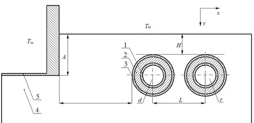
A channel-free heat pipeline is operated in the real application conditions (There is a heated basement of a building). Figure1shows a scheme of decision domain.
For the domain under consideration (Fig.1) we solve a 2D linear and stationary problem of heat transfer in conditions of an engineering structure effect. Formulating the problem, we used the following
Figure 1. A scheme of decision domain: 1 – metal wall of the heat pipeline; 2 – insulating layer; 3 – waterproofing layer; 4 – ground; 5 – engineering structure (heated basement of a building); d, r – direct and return heat pipelines; H – distance from the ground surface to the upper layers of waterproofing points; L – distance between axes of heat pipelines; A – deep of foundations; B – distance from the tip of the heat pipeline to the engineering structure.
assumptions:
1. The heat transfer processes in the internal and the external environment are disregarded. 2. Thermophysical characteristics of materials used in the analysis are constant and known values. 3. There is an ideal thermal contact conditions at the boundaries.
4. The heat in the decision domain (Fig.1) is transferred only by conduction.
The listed assumptions, on the one hand, do not impose constrains of principle on the physical model of the system (Fig.1), but, on the other hand, allow one to simplify in a certain manner the algorithm and method for solving the posed problem.
3. Mathematical model
In the proposed statement, the heat transfer process in the considered decision domain (Fig. 1) in a general formulation is described:
∇2Td
,p =0, (1)
∇2T
r,p =0, (2)
∇2Td
,i =0, (3)
∇2Tr
,i =0, (4)
∇2T
d,h=0, (5)
∇2T
∇2Tg =0, (7)
∇2Tf =0. (8)
Td,p,1=Td =const, (9)
Tr,p,1=Tr=const. (10)
pgrad(Td,p,2)=igrad(Td,i,2);Td,p,2=Td,i,2, (11)
pgrad(Tr,p,2)=igrad(Tr,i,2);Tr,p,2=Td,i,2, (12)
igrad(Td,i,3)=hgrad(Td,h,3);Td,i,3=Td,h,3 (13)
igrad(Tr,i,3)=hgrad(Tr,h,3);Tr,i,3=Tr,h,3, (14)
hgrad(Td,h,4)=ggrad(Td,g,4);Td,h,4=Td,g,4, (15)
hgrad(Tr,h,4)=ggrad(Tr,g,4);Tr,h,4=Tr,g,4, (16)
ggrad(Tg,5)=fgrad(Tf,5);Tg,5=Tf,5. (17) −ggrad(Tg,6)=6(Tg,6−Tex), (18) −fgrad(Tf,7)=7(Tf,7−Tin), (19) −fgrad(Tf,8)=8(Tf,8−Tin), (20) −fgrad(Tf,9)=9(Tf,9−Tex). (21)
grad(Tg)=0,x → ±∞;y → −∞, (22)
grad(Tf)=0,x → −∞;y → +∞. (23)
4. Method of solution and initial data
The system of Eqs. ((1)–(23)) was solved by the finite element method [12], using the Galerkin approximation [13]. The investigations were carried out on a nonuniform finite-element mesh having 18038 nodes and 36015 elements. The number of elements was chosen from conditions of convergence of solution, the mesh was made denser by the Delaunay method [12,13].
In spite of the fact that in statement of the problem it was assumed to use an infinite-size domain (Eqs. (22) and (23)), in the numerical analysis of heat loss we used a calculation domain of 7 m in depth and 8 m laterally from the symmetry axis. The sizes of the calculation domain were chosen on the basis of a series of preliminary numerical experiments in such a manner that the relative change of the temperature gradients at the domain boundary does not exceed 0.5%.
Table1contains values [10,11] of thermophysical characteristics, which were used in the numerical investigations of thermal conditions of the system under consideration (Fig.1).
Table 1. Thermophysical characteristics.
Material Waterproofing layer Insulating layer Metal wall of Ground Foundation
the heat pipeline (reinforced concrete)
, [W/(m·K)] 0.33 0.033 50.2 1.5 1.54
c, [J/(kg·K)] 2200 1470 462 1150 887
, [kg/m3] 920 50 7700 1960 2200
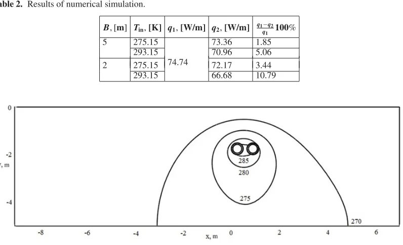
Table 2. Results of numerical simulation.
B, [m] Tin, [K] q1, [W/m] q2, [W/m] q1−q2
q1 100%
5 275.15 73.36 1.85
293.15 70.96 5.06 74.74
2 275.15 72.17 3.44
293.15 66.68 10.79
Figure 2. Temperature field of the ground in the region of channel-free heat pipeline.
The distances from the ground surface to the upper layers of waterproofing points and between axes of heat pipelines wereH =1.5 m andL=0.65 m (Fig.1). The deep of foundations wasA=2 m and the distances from the tip of the heat pipeline to the engineering structure were equalB =2 and 5 m (Fig.1).
The temperature of the inner surface of pipes wereTd =338.15 K andTr =323.15 K. The ambient temperature was Tex =264.35 K. The air temperature inside the engineering structure was equal to Tin=275.15 and 293.15 K. The coefficients of heat transfer in all variants of the numerical analysis were6 =15 W/(m2·K);7=8.7 W/(m2·K);8=4.5W/(m2·K) and9=23W/(m2·K).
5. Results of numerical simulation
The main results of numerical modeling of thermal conditions of the system under consideration (Fig.1) are listed in Table2and in Figs.2–4.
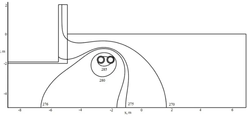
Figure 3. Temperature field of the ground in the region of channel-free heat pipeline (B=2 m,Tin=275.15 K).
Figure 4. Temperature field of the ground in the region of channel-free heat pipeline (B=2 m,Tin=293.15 K).
Table2lists the results of numerical experiments of the heat loss of channel-free heat pipeline in the real application conditionsq2 (There is a heated basement of a building) andq1 (There isn’t a heated basement of a building).
The numerical experimental results in Table2allow us to make the inference about the expected decrease of the heat loss of channel-free heat pipeline with growing air temperature inside the engineering structure Tin and the distances from the tip of the heat pipeline to the engineering structure B. The heat loss of channel-free heat pipeline q2 decrease from 1.85 to 10.79% compared with the heat loss q1.
It was found that the isothermal lines (Figs.2–4) become denser near the ground surface immediately above the heat pipeline and the engineering structure and are sparser as the distance from the heat pipeline and the engineering structure grows; this represents the real operation conditions of the heat pipeline system and qualitatively complies with results of investigations represented in [9,10].
6. Conclusion
We have carried out numerical analysis of thermal regimes and numerical analysis of heat loss of channel-free heat pipeline in the real application conditions (There is a heated basement of a building). It has been shown that application of the proposed approach enables comprehensive analysis of thermal regimes of the system under consideration.
This work was supported by the Grants Council (under RF President), grant No. MK-1652.2013.8, by the Russian Fond of Basic Research, grant No. 12-08-00201 and by the research state assignment “Science” (Code of Federal Target Scientific and Technical Program 2.1321.2014).
Notations
T – temperature, K; – thermal conductivity, W/(m·K); c– heat capacity, J/(kg·K); – density, kg/m3;– heat transfer coefficient, W/(m2·K).
Indices:d– direct heat pipeline;r–return heat pipeline;p– pipe;i– insulation;h– waterproofing; g – ground; f – foundation; in – internal; ex – external; 1 – inner surface of the pipe; 2 – 9 partition of borders: “pipe – thermal insulation”, “thermal insulation – waterproofing”, “waterproofing – ground”, “ground – foundation”, “ground – environment”, “inner surface of the wall – air inside the engineering structure”, “floor surface – air inside the engineering structure”, “outer surface of the wall – environment”.
References
[1] B. Rezaie, M.A. Rosen, District heating and cooling: Review of technology and potential enhancements, Applied Energy. 93 (2012) 2–10
[2] D. Magnusson, Swedish district heating – A system in stagnation: Current and future trends in the district heating sector, Energy Policy. 48 (2012) 449–459
[3] D.J.C. Hawkey, District heating in the UK: A Technological Innovation Systems analysis, Environmental Innovation and Societal Transitions. 5 (2012) 19–32
[4] E. Fahlén, E.O. Ahlgren, Accounting for external costs in a study of a Swedish district–heating system – An assessment of environmental policies, Energy Policy. 38 (2010) 4909–4920 [5] K. Comakli, B. Yuksel, O. Comakli, Evaluation of energy and exergy losses in district heating
network, Applied Thermal Engineering. 24 (2004) 1009–1017
[6] A. Dalla Rosa, Í. Li, S. Svendsen, Method for optimal design of pipes for low– energy district heating, with focus on heat losses, Energy. 36 (2011) 2407–2418
[7] G.V. Kuznetsov, V.Yu. Polovnikov, Numerical simulation of the thermal state of a flooded pipeline taking into account unsteadiness of the process of heat insulation saturation with moisture, Thermal Engineering. 55 (2008) 426–430
[9] G.V. Kuznetsov, V.Yu. Polovnikov, Numerical Investigation of Thermal Regimes in Twin– Tube–Channel Heat Pipelines Using Conductive–Convective Model of Heat Transfer, Thermal Engineering. 59 (2012) 310–315
[10] G.V. Kuznetsov, V.Yu. Polovnikov, The conjugate problem of convective–conductive heat transfer for heat , Journal of Engineering Thermophysics. 20 (2011) 217–224
[11] V.Yu. Polovnikov, E.V. Gubina, Heat and Mass Transfer in a Wetted Thermal Insulation of hot Water Pipes Operating Under Flooding Conditions, Journal of Engineering Physics and Thermophysics. 87 (2014) 1151–1158
[12] A.L. Garcia, Numerical methods for physics, Prentice Hall, New York, 2000.