Corresponding author: Jaroslav Štigler: [email protected]
Characteristics of the T-junction with the equal diameters of all branches
for the variable angle of the adjacent branch
Jaroslav Štigler1,a, Roman Klas1 and OldĜich Šperka1
1
Brno University of Technology, Faculty of Mechanical Engineering, Victor Kaplan’s Department of Fluid Engineering, Technická 2896/2, 616 69, Brno, Czech Republic
Abstract. Basic aim of this paper is to bring out the characteristics of the T-junctions. T-junction consists of the one straight pipe and the adjacent branch which can be inclined under various angle Ȗ. These characteristics were done for the T-junctions with equal diameters of all branches and for five different angles of the adjacent branch. There is also included comparison between characteristics obtained by the numerical calculation and by the experiment in this paper.
1 Introduction
The T-junction is a small, but very important part of the pipe-line system. It can vary in shape and it is primarily used for dividing or combining of flow in pipeline. However the T-junction can be also used for mixing of two different liquids, liquid and gas or two different gasses. It can also be used as a simple pump which is called ejector, but this is special case of the T-junction.
The question is how to mathematically describe the T-junction. It is easy to find and use mathematical models of the flow in parts of pipe systems as for instance valves, elbows, diffusors or contractions and other fittings. It is easy because there is one entrance and one exit. Therefore measuring of energy loss coefficients is not difficult. It is more complicated in case of T junction because there are three branches it means there are two entrances and one exit in case of combining flow or one entrance and two exits in case of dividing flow.
2 Mathematical models of T-junction
The history of building up of mathematical models is long. There are some approaches how to model fluid flow in the T-junction. For each mathematical model are consequently defined coefficients which describe the T-junction. Probably the most known book was written by Miller [1]. He set up basic concept of the T-junction mathematical model. The marking of the T-junction branches by Miller is depicted in the figure 1. He defined two coefficients K31 and K32 for dividing flow and K13 and K23 for combining flow.
Figure 1. Marking of T-junction braches by Miller
g
v
h
g
v
h
g
v
K
.
2
.
2
.
2
2 3 1 2 1 3 2 3 31¸¸¹
·
¨¨©
§
+
−
¸¸¹
·
¨¨©
§
+
=
(1)g
v
h
g
v
h
g
v
K
.
2
.
2
.
2
2 3 2 2 2 3 2 3 32¸¸¹
·
¨¨©
§
+
−
¸¸¹
·
¨¨©
§
+
=
(2)g
v
h
g
v
h
g
v
K
.
2
.
2
.
2
2 3 3 2 3 1 2 1 13¸¸¹
·
¨¨©
§
+
−
¸¸¹
·
¨¨©
§
+
=
(3)DOI: 10.1051/
C
Owned by the authors, published by EDP Sciences, 2014 , 0 2110 (2014)
/2 01
67
epjconf EPJ Web of Conferences
4 6 702110
g
v
h
g
v
h
g
v
K
.
2
.
2
.
2
2 3 3 2 3 2 2 2 32¸¸¹
·
¨¨©
§
+
−
¸¸¹
·
¨¨©
§
+
=
(4)The quantities v1, v2, v3 are mean velocities at each branch and h1, h2, h3 are static pressure heads after subtraction of the friction losses at each branch.
The problem of this mathematical model is that these coefficients have no any physical meaning. They are not loss coefficients, because their values can be less than zero.
The problem is that these coefficients are evaluated jus from the unit kinetic energy and unit pressure energy. Unit energy means energy per one kilogram. These coefficients do not respect the flow rate ratio in branches. There was some effort to improve this concept, for example [2, 3],
3 New mathematical model of T-junction
A new mathematical model has been developed by the authors of this paper for long time. First paper where the new mathematical model of T-junction with angle 90° of the adjacent branch was presented in paper [4,5]. Then it was improved for an arbitrary angle of the adjacent branch in [6]. This mathematical model is general so it is also possible to apply it for an unsteady fluid flow in T-junction. The discussion about the problems of unsteady fluid flow in the T-junction is presented in [7]. Many numerical calculation of fluid flow in T-junction was carried out for example [8, 9]. The fluid flow in T-junction was also measured by PIV. The technique of PIV measurements is described in [10, 14]. The comparison of velocity profiles measured by PIV in T-junction branches with numerical calculations is described in [11]. First curves of the new mathematical model coefficients are presented in [12, 13].
Now it will be useful to say a few words about the new mathematical model of T-junction and about its coefficients. Some variables are depicted in the figure 2.
Figure 2. Marking of T-junction branches and variables of a new mathematical model
The marking of branches a, b, c is fixed. The adjacent branch is always marked by letter c. The part of straight pipe, to which the angle of adjacent branch c is measured,
is marked by letter b. The last branch is marked by letter a.
New mathematical model consists of three equations, power equation, momentum equation and equation of continuity. This model respects the flow rate ratio at each branch, orientation of the T-junction against gravity acceleration and it is, in general form, derived for the unsteady fluid flow in T-junction.
The mathematical model presented here is the simplified version for the steady flow and the horizontal T-junction location. This was also described in the [13] where the results for the T-junction with the area aspect ratio 2.4 were published.
So the Power equation under these assumptions can be written in the form
0
.
2
1
.
.
2
.
.
2
.
.
2
2 2 ) ( 2 2 2 2 2 2=
+
¸¸¹
·
¨¨©
§
+
+
¸¸¹
·
¨¨©
§
+
+
¸¸¹
·
¨¨©
§
+
mX X mX P mc c c mc mb b b mb ma a a maQ
A
Q
Q
p
A
Q
Q
p
A
Q
Q
p
A
Q
ρ
ξ
ρ
ρ
ρ
(5)The momentum equation has a form
0
.
.
.
.
.
.
.
2 2 2 2=
+
¸¸¹
·
¨¨©
§
+
+
¸¸¹
·
¨¨©
§
+
+
¸¸¹
·
¨¨©
§
+
X mX M c c c c mc b b b b mb a a a a maA
Q
A
p
A
Q
A
p
A
Q
A
p
A
Q
ρ
ρ
ρ
ρ
ȟ
n
n
n
(6)The last one is the equation of continuity
0
=
+
+
mb mcma
Q
Q
Q
(7)Some comments have to be mentioned to the previous equations.
Variables Qma, Qmb, Qmc represent a mass flow rates in particular branch. The direction of flow is expressed by the mass flow rate sign. The sign is minus in case of the inflow, whereas the sign plus is used in case of outflow.
Variables Aa, Ab, Ac, represent the areas of the cross-sections of particular branch. All three branches have the same diameter it means that all cross-section areas are the same.
Variables pa, pb, pc represent the static pressures at the cross-sections Aa, Ab, Ac. The problem arises here in case of comparison of static pressures obtained from numerical calculations and experimental results. The static pressure is calculated as an area-weighted value over a cross-section area in case of numerical calculations, but in case of experiment the static pressure is measured as an area-weighted value over the pipe perimeter. The slight difference can be between this two pressure values.
Vectors na, nb, nc are the outward unit vectors of the cross-sections Aa, Ab, Ac. Their magnitudes are 1. They are perpendicular to the cross-sections and their orientations are out of the T-junction zone.
There are two variables QmX and AX with strange subscript X in the equations (5) and (6). The subscript X has to be replaced by a letter a or b or c. Which letter is chosen depends on which branch the complete flow rate is flowing through. If the complete flow rate is flowing through branch a so the subscript X is replaced by the letter a and similarly for the other branches b and c.
3.1 Coefficients of T-jucntion
There are two coefficients in the equations (5) and (6). Coefficient ȟP, in the power equation (5), is rate of the total energy losses in the T-junction. It is possible to call it the total power coefficient. This is a scalar quantity from a mathematical point of view. The coefficient ȟM, in the momentum equation, is a rate of force which the fluid is acting on the T-junction. This coefficient is the vector quantity from the mathematical point of view and it is possible to call it total momentum coefficient. The only component in direction of the main pipe (nb direction) will be taken into consideration for this case of the T-junction. Other components of this coefficient are necessary in case when the branches of junction do not lay at one plain or in a case of a cross junction. The component of the momentum equation (6) in direction of vector nb can be obtained by multiplying of this equation by the vector nb. Then this component momentum equation has a form
0
.
cos
.
.
.
.
.
.
.
2 2 2 2=
+
¸¸¹
·
¨¨©
§
+
+
¸¸¹
·
¨¨©
§
+
+
¸¸¹
·
¨¨©
§
+
−
X mX Mb c c c mc b b b mb a a a maA
Q
ȟ
A
p
A
Q
A
p
A
Q
A
p
A
Q
ρ
γ
ρ
ρ
ρ
(8)Variable Ȗ is the angle between branch a and b. Variable ȟMb is the component of the total momentum coefficient in direction of branch b. The coefficients ȟP andȟMb can be obtained from the numerical solution of fluid flow in T-junction or from the experiment. These total coefficients include both influence of friction and influence of shape of the T-junction. The problem of the total coefficients is that they are dependent on the distances of the cross-sections Aa, Ab, Ac from the center of T-junction. This is caused by the friction influence. Therefore it should be good idea to eliminate the friction influence. The idea how to reach this is that the total coefficients will be divided into two parts.
PG PF
P
ȟ
ȟ
ȟ
=
+
(9)
MGb MFb
Mb
ȟ
ȟ
ȟ
=
+
(10)The ȟPG and ȟMGb are the parts which represent the influence of the T-junction shape (geometry). These parts would have been independent of the scale of the T-junction. The only problem is that the momentum coefficients depend on the absolute values of the static pressures pa, pb, pc. This will be discussed later.
The ȟPF and ȟMFb are parts of the total coefficients which represent the influence of the friction. These friction coefficients are possible to express on the basis of known pressure drop in straight pipe for given diameter and mass flow rate. The friction coefficients, under assumptions mentioned at the paper beginning, can be expressed this way
(
)
mX mX X c c c b b b a a a PFQ
Q
S
L
Q
p
L
Q
p
L
Q
p
2
.
.
.
.
.
.
2 2 2 2 1 2 1 2 1ρ
ξ
Δ
+
Δ
+
Δ
=
(11)(
)
2 1 1 1.
.
.
.
.
.
.
.
.
.
.
.
.
.
mX X c c c c c b b b b b a a a a a MFQ
A
A
L
Q
p
A
L
Q
p
A
L
Q
p
ρ
n
n
n
ȟ
Δ
+
Δ
+
Δ
=
(12)Variables La, Lb, Lc are the length of the T-junction branches.
Variables ǻp1a, ǻp1b, ǻp1c are the pressure differences per one meter of pipe length and per one cubic meter per second flow rate. It can be expressed by this formula for particular branch x x x x
Q
L
p
p
.
1Δ
=
Δ
(13)The letters x has to be replaced by the letter of a, b or c in case of particular branch.
The friction momentum equation (12) is a vector equation. In our case we need only component of the friction momentum coefficient in direction of vector nb. This component will be obtained by multiplying this equation by the vector nb.
(
)
2 1 1 1.
.
cos
.
.
.
.
.
.
.
.
.
.
mX X c c c c b b b b a a a a MFbQ
A
A
L
Q
p
A
L
Q
p
A
L
Q
p
ȟ
ρ
γ
Δ
+
Δ
+
Δ
−
=
(14)The total coefficients can be obtained from measurements. We have to measure static pressures and flow rates at each branch.
After that the friction coefficients can be also calculated. The values of ǻp1a, ǻp1b, ǻp1c can be obtained either by experimental way or by using some empirical formula for friction losses in the straight pipe. They were measured before the measurement of the T-junction started. In case of numerical solution they are evaluated from the numerical solution.
Then the geometrical coefficients can be evaluated from the equations (9) and (10).
PF P PG
ȟ
ȟ
ȟ
=
−
(15)
MFb Mb
MGb
ȟ
ȟ
ȟ
=
−
(16)The only problem is that total momentum coefficient
ȟMb depends on the absolute pressure values. Therefore one of the static pressures has to be used as the reference pressure with value 0 to be able to compare the experimental results. The differences between static pressures pa, pb, pc remain unchanged. For example if the chosen reference pressure is pa then pa = 0, pb = pb - pa,
pc = pc - pa.
This does not influence the total power coefficient
ȟPG, but the total momentum coefficients will be comparable.
4 Experiment
Main goal of this paper is to present results of experiments and its comparison with the numerical modeling. Previous chapters were written to help reader to understand basic ideas of the new mathematical model and the T-junction coefficients definitions.
The experiment was carried out in the laboratory of Victor Kaplan’s Department of Fluid Engineering at the Brno University of technology Faculty of Mechanical Engineering.
As it was mentioned before the diameters of all three T-junction branches were the same and it was 50mm. The T-junction was made by drilling of holes into the plastic block. The measurements were performed for five different angles of the adjacent branch. (Ȗ = 30°, 45°, 60°, 75°, 90°). The six different flow configurations were measured for each of the T-junction geometry. Three of them are for flow dividing and three of them are for flow combining. These flow configurations are shown in the figure 3 for better understanding. Eleven different ratio of flow rates were measured for each flow configuration.
Dividing flow configuration
Combining flow configuration
Figure 3. Different flow configuration
The measurements were performed on the open test circuit. The diagram of the test circuit is in the figure 4. There was measured static pressure at one branch of T-junction (pa). Then the two pressure differences between this branch and the other two branches were measured (ǻpab, ǻpab). Pressure differences were measured simultaneously by the differential manometers and by the U-tube manometers. The flow rates were measured at each branch by the magnetic flow meters (FMa, FMb, FMc). The flow rates were controlled by the variable-frequency drive applied on the pump electric motor and by the regulating valves. The temperature of water (TM) was also measured.
Measurement of the one flow configuration was performed twice. The time delay between these measurements of one flow configuration was at least one day.
Figure 4. Diagram of the test circuit.
5 Numerical calculations
The geometries of the T-junctions were created in the pre-processor GAMBIT 2.2.30. The lengths of all branches, measured from the border of junction area, were 25 of pipe diameters. The condition “wall” was used on a pipe walls. The condition “velocity inlet” was applied on the pipe cross-sections where the fluid was entering the pipe system. The condition “outflow” was used on the pipe cross-sections where the fluid was leaving the pipe system. The mesh was created from the hexahedral cells. The number of cells was approximately 2.3 million. The worst cell skewness was 0.51. Used turbulence model was k-İ realizable with non-equilibrium wall functions. The problem was solved as a unsteady fluid flow. For each flow configuration was solved 21 different flow ratios.
6 Discussions
The results obtained by the experiments and their comparison with the numerical calculations will be discussed in this chapter. The geometry coefficients for all cases of flow configurations and for all angles of adjacent branch as a function of flow rate ratio (q) are drawn in figures 5-16 at the end of this paper. Ratios of different branch flow rates are used for particular flow configuration.
from the data for flow configuration Div b (Com b) for the angles in interval 30°-75° and contrariwise. In case of “Div c” (“Com c”) it is possible to obtain the curves for angles in interval 75°-150° by the exchange of the data of branch a and branch b for angles 30°-75°.
The single points represent the data obtained from measurements in the graphs. The lines represent data obtained from the numerical modeling. The solid lines are used for the data directly calculated or measured (it is for the angles in interval 30°–75°). The dashed lines means that this curves are converted from the data of the other flow configuration (it is for the angles in interval 105°-150°).
It is possible to say that if the curves for whole range of adjacent branch angle (30°-150°) are known in case of flow configuration “Div a” or “Com a” then the curves for the flow configuration “Div b” or “Com b” can be converted from the previous one. The results for the particular flow configurations will be discussed in the next chapters.
6.1 Dividing flow Div a
The flow rate ratio in case of flow configuration “Div a” is defined this way
a c ca
Q
Q
q
=
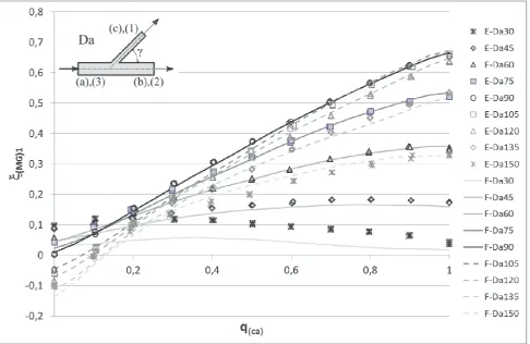
(17)The geometry coefficients as a function of qca are drawn in figures 5 and 6. The data obtained from the numerical calculations and from the measurement are in a good agreement. The measured geometry power coefficients for adjacent branch angles 30°, 45°, 135° and 150° are slightly higher than the calculated coefficients. The curves of the geometry momentum coefficients obtained from the experiment are also in good agreement with the curves obtained from the numerical solution of the fluid flow. It is interesting that the highest geometry momentum coefficients are for the 90° inclination of the adjacent branch. These coefficients for the angle of adjacent branch higher than 90° for qca < 0.1 are negative. It is because pressures in the adjacent branch are very low. The water is sucked out of the adjacent branch into the main stream. The T-junction works in this case as an ejector.
6.2 Dividing flow Div b
The flow rate ratio in case of flow configuration “Div b” is defined this way
b c cb
Q
Q
q
=
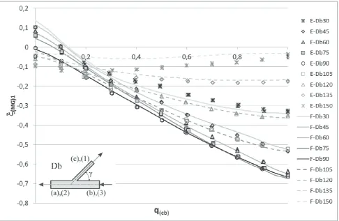
(18)The curves of the coefficients for this flow configuration are drawn in the figures 7 and 8. Description of these coefficients is very similar to the coefficients of flow configuration “Div a” because they can be converted from the coefficients of flow configuration “Div a”.
6.3 Dividing flow Div c
The flow rate ratio in case of flow configuration “Div c” is defined this way
c a ac
Q
Q
q
=
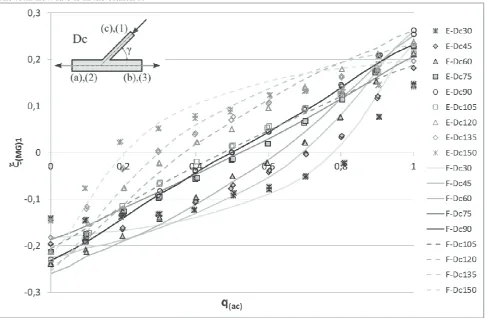
(19)The curves of the coefficients for this flow configuration are drawn in the figures 9 and 10. The differences between power coefficients obtained from experiment and from numerical solution of fluid flow are higher in this case. The coefficients from experiment are higher than the coefficients from the numerical solution. There is very high turbulence in the region of the flow division therefore it is difficult to model such fluid flow. There is one interesting phenomenon that all curves of geometry power coefficient obtained from experimental data are crossing at one point for flow rate ratio qac=0.5 with value ȟPG =1. The geometry momentum coefficients are smaller in comparison with the case of flow configuration “Div a” and “Div b”. There is good agreement between the experimental data and data from numerical solution in the tendency of the curves.
6.4 Dividing flow Com a
The flow rate ratio in case of flow configuration “Div c” is defined this way
a c ca
Q
Q
q
=
(20)The curves of the coefficients for this flow configuration are drawn in the figures 11 and 12. Generally the agreement between experimental data and data obtained from numerical solution of fluid flow is better in case of dividing flow. The curves of geometry power coefficient are very similar to the ones for the dividing flow. But the geometry momentum coefficients are very high. The agreement between experimental and numerical data is very good in this case. The geometry momentum coefficients are lesser then then zero for the angle of adjacent branch smaller than 90°.
6.4 Dividing flow Com b
The flow rate ratio in case of flow configuration “Div c” is defined this way
b c cb
Q
Q
q
=
(21)geometry momentum coefficients are symmetrical around the zero value of geometry momentum coefficient.
6.4 Dividing flow Com c
The flow rate ratio in case of flow configuration “Div c” is defined this way
c a ac
Q
Q
q
=
(22)The curves of the coefficients for this flow configuration are drawn in the figures 15 and 16. The agreement between data obtained from the experiment or from the numerical solution is very good in this case.
The curves of the geometry power coefficients do not cross at one point on the contrary to the flow configuration “Div c”. The curves of geometry momentum coefficients are almost linear.
7 Conclusions
The new mathematical model of T-junction was presented in this paper. The definitions of the T-junction coefficients with clear physical meanings were carried out. The geometrical coefficients obtained from experiment and from numerical solution were presented here. The comparison between experimental data and the data obtained on the basic numerical solution was performed. This mathematical model can be used for solution of fluid flow in pipe systems and also for comparison of the different shapes of the T-junctions.
8 Acknowledgement
This research was funded by Grant Agency of Czech Republic (GACR) under project “Mathematical and
Numerical Modeling of Flow in Pipe Junction and its Comparison with Experiment” with registration number 101/09/1539 and by Brno University of Technology, Faculty of Mechanical Engineering under project with the number FSI-S-12-2.
9 References
1. D. S. Miller, Internal flow, A guide to losses in pipe and duct systems,
2. K. Oka, H. Ito. J Fluid Eng. 127, 110, (2005)
3. J. Pérez-García, E. Sanmiguel-Rojas, A. Viedma, Applied Mathematical Modeling. 34, 4289, (2010) 4. J. Štigler, J. Mech. Eng. 5,249-262, (2006) 5. J. Štigler, J. Mech. Eng. 5,263-270, (2006)
6. J. Štigler, IOP Conf. Ser.:Earth Environ. Sci., 12, 12101, (2010)
7. J. Štigler, Scientific Buletin of the “Politechnica” University of Timisoara, Romania Transactions on Mechanics, 6, 83-92, (2007)
8. L. Beneš, P. Louda, R. Keslerová, J. Štigler, J. Amc.,
04,074, (2011), (In press)
9. P. Louda, K. Kozel, J. PĜíhoda, L. Benes, J. Compfluid., 12, 003, (2010)
10. M. Kotek, V. Kopecký, D. Jašíková, Recent Researches in Mechanics, Proc. of the 2nd International Conference on Fluid Mechanics and Heat and Mass Transfer 2011 (FLUIDSHEAT11) WSEAS Cofru,169-172, (2011)
11. J. Štigler, R. Klas, M. Kotek, V. Kopecký, J. Proeng., 39, 19-27, (2012
12. J. Štigler, O. Šperka, R. Klas, Eng. Mech. 2011, 607-610, (2011)
13. J.Štigler, O.Šperka, EPJ Web of Conferences 45,
01112 (2013)
T-junction coefficients for dividing flow - Div a
Figure 5. The geometry power coefficient ȟPGas a function of the flow rate ratio qca in case of the dividing flow (Da). The total flow rate is in the branch a.
Figure 6. The geometry momentum coefficients ȟMGbas a function of the flow rate ratio qca in case of the dividing flow (Da). The total flow rate is in the branch a. The reference pressure is pa=0.
T-junction coefficients for dividing flow - Div b
Figure 7. The geometry power coefficient ȟPGas a function of the flow rate ratio qcb in case of the dividing flow (Db). The total flow rate is in the branch b.
T-junction coefficients for dividing flow - Div c
Figure 9. The geometry power coefficient ȟPGas a function of the flow rate ratio qac in case of the dividing flow (Dc). The total flow rate is in the branch c.
Figure 10. The geometry momentum coefficients ȟMGbas a function of the flow rate ratio qac in case of the dividing flow (Dc). The total flow rate is in the branch c. The reference pressure is pc=0.
T-junction coefficients for combining flow - Com a
Figure 11. The geometry power coefficient ȟPGas a function of the flow rate ratio qca in case of the combining flow (Ca). The total flow rate is in the branch a.
T-junction coefficients for combining flow - Com b
Figure 13. The geometry power coefficient ȟPGas a function of the flow rate ratio qcb in case of the combining flow (Cb). The total flow rate is in the branch b.
Figure 14. The geometry momentum coefficients ȟMGbas a function of the flow rate ratio qcb in case of the dividing flow (Cb). The total flow rate is in the branch b. The reference pressure is pb=0.
T-junction coefficients for combining flow - Com c
Figure 15. The geometry power coefficient ȟPGas a function of the flow rate ratio qac in case of the combining flow (Cc). The total flow rate is in the branch b.