Article
1
An analytical Modeling for Designing the Process
2
Parameters for Temperature Specifications in
3
Machining
4
Elham Mirkoohi 1*, Peter Bocchini 2, and Steven Y. Liang 1
5
1 Woodruff School of Mechanical Engineering, Georgia Institute of Technology, Atlanta, GA 30332, USA;
6
7
2
Boeing Research and Technology, Huntsville, AL, 35824, USA
;
[email protected]8
* Correspondence: [email protected]
9
10
Abstract: Different process parameters can alter the temperature during machining. Consequently,
11
selecting process parameters that lead to a desirable cutting temperature would help to increase the
12
tool life, decrease the tensile residual stress, and controls the microstructure evolution of the
13
workpiece. An inverse computational methodology is proposed to design the process parameters
14
for specific cutting temperature. A physics-based analytical model is used to predict the
15
temperature induced by cutting forces. To calculate the temperature induced by the deformation in
16
the shear zone, a moving point heat source approach is used. The shear deformation and chip
17
formation model is implemented to calculate machining forces as functions of process parameters,
18
material properties, and etc. The proposed model uses the analytical model to predict the cutting
19
temperatures and applies a variance-based recursive method to guide the inverse analysis. In order
20
to achieve the cutting process parameters, an iterative gradient search is used to adaptively
21
approach the specific temperature by the optimization of process parameters such that an inverse
22
reasoning can be achieved. Experimental data are used to illustrate the implementation and
23
validate the viability of the computational methodology.
24
Keywords: Inverse analysis; Temperature prediction; Process parameters; Cutting speed; Depth of
25
cut
26
27
1. Introduction
28
Temperature measurement and prediction have been a major focus of machining research for
29
several decades [1, 2]. Temperature generation during machining has a substantial effect on the tool
30
wear, tool distortion, residual stress, and microstructure evolution of the workpiece. During cutting
31
metals, a considerable amount of the input power is transferred into heat through plastic deformation
32
of the workpiece material, the friction of the chip on the tool and the friction between the tool and the
33
workpiece. The heat generated in the cutting zone can influence the cutting tool and the of the
34
workpiece qualities [3].
35
The dissipated heat can considerably change the microstructure of the workpiece. Cutting
36
process parameters such as cutting speed, feed rate, and depth of cut have a substantial influence on
37
machining temperature. Increase in cutting temperature results in greater tensile residual stress on
38
the surface of a machined component [4]. As a result, choosing viable cutting process parameters can
39
significantly help to have a desired cutting temperature.
40
Many works have been done in determining the temperature distribution in machining. In the
41
past few decades, numerical methods, such as finite element method (FEM) is utilized for the
42
temperature prediction in machining since it provides a better understanding of the heat generation
43
in the cutting zone, resulting stresses, temperature fields, and chip formation mechanisms. Lei et al.
44
developed a thermomechanical two-dimensional FE model for the orthogonal cutting process with
45
continuous chip formation [5]. Umbrello et al. developed a FE model to predict temperature when
46
steady-state conditions were reached. Pure thermal simulation is conducted in order to determine
47
the heat transfer coefficient between tool and workpiece in steady-state condition. The obtained heat
48
transfer coefficient was used in a thermomechanical simulation for temperature prediction [6]. Özel
49
et al. developed a FE model to investigate the influence of cutting-tool edge roundness on the
50
temperature field at tool–chip and tool–workpiece interfaces [7].
51
Many researches developed analytical models to predict the temperature in machining process.
52
Komanduri et al. developed an analytical model for temperature prediction. The obtained
53
temperature is combined effects of the shear plane heat source at the primary shear zone and the
54
frictional heat source at the secondary shear zone [8]. Liang et al. developed a physics-based
55
analytical model to predict temperature distribution by considering the tool thermal properties and
56
the tool wear effects [9]. Huang et al. developed a cutting temperature model with an assumption of
57
non-uniform heat intensity and partition ratio and reported improved accuracy upon validation [10].
58
Considerable accuracy is achieved from the FEM, but computational efficiency is low. On the
59
other hand, the analytical model provides accurate results. The high computational efficiency and
60
easy implementation are the other advantages of the analytical models for the machining process
61
modeling [11, 12].
62
The process parameters need to be selected in order to achieve a desirable temperature in
63
machining. Randomly choosing the process parameters and predicting the cutting temperature
64
through analytical model or finite element analysis repeatedly is not a reasonable way to achieve a
65
desirable temperature during machining. Nowadays, most of the researchers are using the trial and
66
error method in order to have a desirable workpiece performance. This method is not only time
67
consuming, but also expensive. As a result, an inverse analysis is proposed in addition to the forward
68
analysis to identify the viable solutions of process parameters that can achieve a specific performance.
69
An inverse analysis is successfully used for identification of mechanical properties which are
70
hard to be measured in experiments [13-16]. Pujana et al. used an inverse analysis to identifies the
71
coefficients of constitutive equations of flow stress in orthogonal cutting and used finite element
72
method to evaluate the results [17]. Denkena et al used the inverse analysis to predict the
73
constitutive parameters of the Johnson-Cook’s flow stress model . [18]. Chen et al. chose cutting force
74
and chip thickness as targets and optimized the inverse analysis of determining Al6063 constitutive
75
model coefficients [19]. Sampsa et al. also used the inverse analysis to predict Johnson-Cook model
76
parameters with four target performances including cutting force, tangential force, resultant force,
77
and cutting temperature [20]. Mirkoohi et al. [21] used an inverse analysis to predict the process
78
parameters in turning of Ti-6Al-4V in order to achieve a desirable cutting force.
79
There are significant works on literature on modeling of the temperature during the machining
80
process. However, the lack of enough research on selecting the viable process parameters which
81
result in a desirable temperature is noticeable. The influence of cutting process parameters on
82
temperature is profound. Therefore, a systematic approach is required to obtain these cutting process
83
parameters. Determining the process parameters to ensure resulting cutting temperature can
84
significantly help to have a desirable workpiece microstructure, and also residual stress [22].
85
In order to achieve desirable cutting temperature, it is required to select the process parameters
86
in a systematic manner. A physics-based model is used to predict the temperature. The heat comes
87
from the primary shear zone and the tertiary shear zone between tool and workpiece. An imaginary
88
moving heat source approach is used to calculate the temperature field induced by the deformation
89
in the shear zone [23] . Next, an iterative gradient search procedure is set up to adaptively approach
90
the specific temperature by the optimization of process parameters such that an inverse reasoning
91
parameters including depth of cut and cutting velocity and achieves the optimal solution for the
93
temperature.
94
To illustrate the implementation method and validate the viability of the proposed method,
95
experimental data are used. These data are used as a starting point for inverse analysis. The proposed
96
model achieves the closest temperature to the experimental temperature by the optimization of
97
process parameters and inversely designs the cutting process parameters such as cutting velocity and
98
depth of cut.
99
2. Approach and Methodology
100
2.1. The Forward Analysis: Temperature Modeling
101
The temperature gradient induced by the cutting process can have a significant effect on the
102
residual stress, tool wear, and microstructure evolution of the workpiece. The increased in cutting
103
temperature in machining result in greater tensile residual stress on the surface of a machined
104
component [24]. In modeling of the workpiece temperature, two heat sources are assumed to exist.
105
The first is the primary heat source generated from the shear zone [25]. The second heat source is a
106
result of rubbing between the tool and the workpiece. To calculate the temperature field induced by
107
the deformation in the shear zone, a moving heat source approach is used. The temperature rises in
108
the workpiece due to shear deformation is the combined effects of the shear heat source and moving
109
heat source [23], which can be obtained as
110
111
∆ ( , ) =
4
( )
×
112
(x − l sinφ) + (z − l cos φ) + (x − l sinφ) + (z + cos φ) dl (1)
113
114
where L is the shear length, =
∅ , ∅ is the shear angle, t is undeformed chip thickness, ∅ =
115
− , is the cutting speed, a is the workpiece thermal diffusivity, is workpiece thermal
116
conductivity, and is the modified second Bessel function. The average shear stress in the shear
117
zone can be approximated as
118
119
q =( )
( ) (2)
120
121
where, F and F are the cutting forces. The cutting forces consist of chip formation and
122
plowing force which can be calculated from shear deformation and chip formation model [26]. In
123
this model, the cutting plane is considered as a thick cutting band. As a result, the effects of material
124
deformation and work hardening can be considered.
125
A moving heat source can also be used to calculate the heat generated in the rubbing zone. To
126
satisfy the insulated boundary condition on the workpiece surface, an imaginary heat source is
127
imposed as coinciding with the original rubbing heat generation. The temperature rise induced by
128
the tool–workpiece rubbing can be calculated as
129
130
∆T (x, z) = × ∫ K exp (−( ) [ (x − s) + (z) ] ds (3)
131
132
where CA is the work-dead zone interface length which is calculated using slip line model [27].
133
γ is heat partition coefficient that transferred to the workpiece. According to Barber [28], the heat
134
partition coefficient could be calculated as
135
γ = (4)
136
where the subscript ρ , Cw, and Kw are the workpiece material density, heat capacity, and
138
thermal conductivity, respectively. ρ , C , and K are corresponding the tool properties.
139
The rubbing stress q is determined from the plowing force P in the cutting direction as
140
141
q = (5)
142
143
The plowing force Pc can be calculated from traditional cutting mechanics [29], and w is the
144
width of cut. The total temperature rise in the workpiece can be obtained by superimposing the two
145
temperature effects from rubbing and shear as
146
147
∆T = ∆T + ∆T (6)
148
149
150
152
2.2. Inverse Analysis: An iterative gradient search based on Kalman filter:
153
The proposed algorithm estimates two unknown cutting process parameters which are the
154
depth of cut ( ) and cutting tool velocity (V) on the basis of experimentally measured cutting
155
temperature. Fig. 1 is demonstrated the proposed approach. The two unknown constants are
156
represented as = ( , ) . At time s = 0, the initial estimates are = ( , ) . These initial
157
estimates of cutting process parameters are used to calculate the initial cutting temperature. Then the
158
obtained cutting temperature is compared to the desired temperature that is assigned at the first of
159
the proposed model.
160
The estimation of subsequent cutting process parameters is obtained as
161
162
X = X + K T − T (X ) (7)
163
164
is the Kalman gain matrix, Texp is the vector containing the experimentally determined
165
temperature in machining. ( ) is the vector containing the cutting temperature computed from
166
the previous iteration using forward model as explained in section 2.1.
167
168
T = [ T ] (8)
169
170
T (X ) = [T ] (9)
171
172
The Kalman gain matrix is computed as
173
174
K = P R (10)
175
176
P = P − P P R × P (11)
177
178
The Kalman gain matrix is multiplied by the differences between the experimental and the
179
iterated temperature to update the unknown depth of cut ( ) and velocity (V), as shown in Eqn. 10.
180
For the two unknown cutting process parameters ( and V) and the known cutting temperature, the
181
size of the Kalman gain matrix is 2×1. ∈ ℝ × contains the gradients of with respect to
182
unknown cutting process parameters. Furthermore, is the simulation covariance matrix, which is
183
the range of the unknowns at increment s, and is the error covariance matrix, which is the size of
184
the simulated error. is updated at each step, whereas is a non-iterative parameter that is
185
prescribed at the initialization stage. Due to the sensitivity of the convergence rate of the Kalman
186
algorithm to the value of and , it is essential that these two matrices be assigned properly. The
187
initial simulation covariance matrix and the error covariance matrix are set to be
188
189
P = ΔV 0
0 Δt (12)
190
191
R = [ T ] (13)
192
193
where, ∆ and Δ state the predicted ranges of the unknown process parameters. In the
194
current analysis, the diagonal components of are chosen on the basis of the experimentally
195
determined cutting temperature. The error threshold is used as stopping strategy for this approach.
196
In each iteration, the error between experimental cutting temperature and predicted is computed. If
197
the less error than the desired error is obtained, the algorithm will be terminated.
198
In order to illustrate the implementation and also to validate the viability of the computational
200
methodology, the orthogonal experimental data are selected from Umbrello et. al. [6]. Two
201
chromel/alumel thermocouples (K-Type) with a diameter of 0.5 mm are embedded in the tool. The
202
temperatures are acquired by an analogical/digital converter. The material in these experiments is
203
AISI 1045 steel. The material properties of AISI 1045 steel is listed in Table 1 [24]. The cutting speed
204
ranging from 50 to 100 m/min. Three different values of depth of cut (0.05, 0.1, 0.15 mm/rev) are used.
205
The rake angle is −10°. The cutting width for all the cases is 3 mm, and the clearance angle is 11°.
206
207
Table 1. Thermal and mechanical properties of AISI 1045
208
209
210
211
212
213
214
215
216
In each loop, both direct analysis and inverse analysis are conducted once, and the predicted
217
temperature is compared to the experimental measurement. By varying the depth of cut, and velocity
218
the temperature data from the experiment, and the proposed model are listed in Table 2. The
219
proposed inverse model tries to change the process parameters in each step in the direction that the
220
model predicts the closest temperature to the desired temperature. The predicted cutting temperature
221
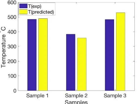
and experimental cutting temperature are plotted in Fig. 2. The experimental cutting temperatures
222
are the desirable values. The predicted cutting temperatures tend to be higher than the experimental
223
values. The maximum error between the experiment and model is for sample 3, which is 9.56%. The
224
main reason for these errors comes from the gap between the analytical model and experimental
225
measurements in the forward analysis.
226
227
228
229
Figure 2. Comparison of predicted cutting temperature with experiments for a rake angle of −10° and
230
different depth of cut and velocity.
231
232
233
234
235
236
237
238
239
Table 2. Comparison of temperature and process parameter
240
241
242
243
244
245
246
247
248
249
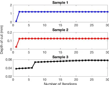
The goal of the proposed model is to design the cutting velocity and depth of cut for a desired
250
temperature. The initial guess = ( , ) is chosen arbitrarily. For the first sample, as shown in
251
Fig. 3 the initial depth of cut is 0.1 mm and it is converged to 1.2 mm after a very short number of
252
iterations. This value is far from the initial specified depth of cut. The cutting velocity is plotted as a
253
function of the number of iterations in Fig. 4. For sample 1, the initial guess is 0.5 m/s and it is
254
converged to 6.07 m/s at a very low number of iterations, which shows the efficiency of the proposed
255
model. This worth to note that for a given temperature, many combination of process parameters can
256
be estimated in order to satisfy the given temperature. The cutting temperature is obtained by
257
optimization of the process parameters, as illustrated in Fig. 5. The optimal solution for sample 1 is
258
489.59°C. The temperature measured from experiment is 485°C.
259
260
261
Figure 3. Evolution of depth of cut as a function of number of iterations.
262
263
For the second sample, the temperature measured from the experiments is 383 °C. This value of
264
temperature is chosen as a desired value. The initial guess is = [1.5, 0.05] . After a very short
265
number of iterations, it is converged to = [4.42, 0.13] . The optimal predicted temperature from
266
the proposed model is 357.44°C.
267
For the third sample, the temperature measured from the experiments is 483 °C. This value of
268
temperature is also chosen as a desired value. The initial guess is = [1.5, 0.05] , and it is converged
269
to = [1.6 , 0.057] . The optimal calculated temperature is 529. 18°C.
270
271
272
Samples 1 2 3 T (exp)/C 485 383 483 T (model)/C 489.59 357.44 529.18 V (exp)m/s 1.66 0.83 0.83 V (model)m/s 6.07 4.42 1.6
273
Figure 4. Evolution of cutting velocity as a function of number of iterations
274
275
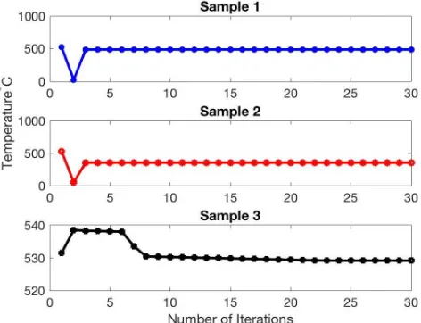
By estimating the process parameters at each iteration for each sample as shown in Fig. 3 and
276
Fig. 4 the temperature during the machining can be obtained using the forward model as explained
277
in section 2.1. The obtained temperature is plotted as a function of number of iterations for each
278
process parameters for all three samples as shown in Fig. 5. In sample 1 and 2, the temperature
279
converges after two number of iterations. In sample 3 the temperature converges after eight number
280
of iterations which shows the efficiency of the proposed model.
281
282
283
284
Figure 5. Evolution of temperature as a function of number of iterations
285
286
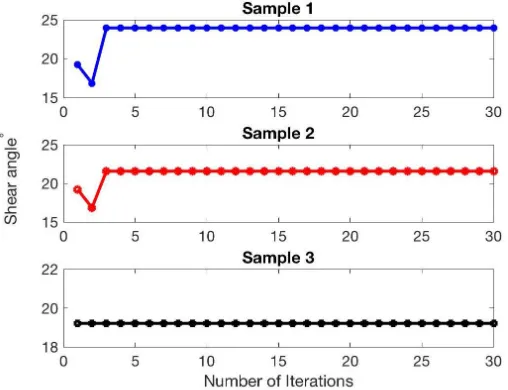
The shear deformation and chip formation model, as proposed by Oxley, is used to predict the
287
cutting forces for a desirable temperature in machining. The cutting force and thrust force are plotted
288
in Fig. 6 and Fig 7. The cutting force and thrust force follow the same trend, and they converge at
289
very short number of iterations. The corresponding shear angle is also plotted in Fig. 8. The shear
290
angle in these three samples has the range between 19° in sample 3 to 24° in sample 1.
291
293
Figure 6. Evolution of cutting force as a function of number of iterations
294
295
296
297
Figure 7. Evolution of cutting force as a function of number of iterations
298
299
300
301
Figure 8. Evolution of shear angle as a function of number of iterations.
302
4. Conclusions
305
A physics-based model along with an iterative gradient search based on Kalman filter algorithm
306
is utilized to determine the cutting process parameters for the desired temperature. Having a
307
desirable temperature in the machining process can significantly reduce the tensile residual stress,
308
tool wear, and it helps to control the microstructure evolution of the workpiece.
309
In order to obtain the desirable cutting temperature, the viable cutting process parameters
310
should be selected. A physics-based model is used to obtain the cutting temperature using an
311
imaginary heat source approach.
312
The gradient search procedure is set up to adaptively approach the cutting temperature by the
313
optimization of process parameters such that an inverse reasoning can be achieved. Experimental
314
data are used to illustrate the implementation and also validate the viability of the computational
315
methodology.
316
The predicted cutting temperature is considerably close to the experimental data. The obtained
317
cutting process parameters are far from the initial assigned process parameters. In other words, the
318
proposed model can obtain the process parameters even when the initial guess is far from the
319
solution. The cutting velocity and depth of cut are converged at a very short number of iterations
320
which shows the efficiency of the proposed model.
321
In each iterative step, a new cutting force, and thrust force are generated which was calculated
322
using shear deformation and chip formation model for a given cutting temperature. Moreover, the
323
shear angle is obtained using an iterative algorithm. The proposed analytical model provides a fast
324
computation of process parameters for a specific temperature without needing costly experiments,
325
and time consuming finite element analysis. Furthermore, selecting viable cutting process parameters
326
which results in a specific cutting temperature, can significantly influence the tool wear, input power,
327
and also can lead to having a desirable microstructure.
328
Author Contributions: E.M. conceived and developed the proposed analytical model, extracted and
329
analyzed the data, and wrote the paper. P.B provided general guidance. S.Y.L. provided general
330
guidance and proofread the manuscript writing.
331
Conflicts of Interest: The authors declare no conflict of interest.
332
References
333
1. Yen, Y.-C., A. Jain, and T. Altan, A finite element analysis of orthogonal machining using different tool
334
edge geometries. Journal of materials processing technology, 2004. 146(1): p. 72-81.
335
2. Sutter, G., et al., An experimental technique for the measurement of temperature fields for the orthogonal
336
cutting in high speed machining. International Journal of Machine Tools and Manufacture, 2003. 43(7): p.
337
671-678.
338
3. Ng, E.-G., et al., Modelling of temperature and forces when orthogonally machining hardened steel.
339
International Journal of Machine Tools and Manufacture, 1999. 39(6): p. 885-903.
340
4. Thiele, J.D., et al., Effect of cutting-edge geometry and workpiece hardness on surface residual stresses in
341
finish hard turning of AISI 52100 steel. Journal of Manufacturing Science and Engineering, 2000. 122(4): p.
342
642-649.
343
5. Lei, S., Y. Shin, and F. Incropera, Thermo-mechanical modeling of orthogonal machining process by finite
344
element analysis. International Journal of Machine Tools and Manufacture, 1999. 39(5): p. 731-750.
345
6. Umbrello, D., et al., On the effectiveness of finite element simulation of orthogonal cutting with particular
346
reference to temperature prediction. Journal of Materials Processing Technology, 2007. 189(1-3): p. 284-291.
347
7. Özel, T. and E. Zeren, Finite element modeling the influence of edge roundness on the stress and
348
temperature fields induced by high-speed machining. The International Journal of Advanced
349
Manufacturing Technology, 2007. 35(3-4): p. 255-267.
350
8. Komanduri, R. and Z.B. Hou, Thermal modeling of the metal cutting process—Part III: temperature rise
351
distribution due to the combined effects of shear plane heat source and the tool–chip interface frictional
352
heat source. International Journal of Mechanical Sciences, 2001. 43(1): p. 89-107.
353
9. Li, K.-M. and S.Y. Liang, Modeling of cutting forces in near dry machining under tool wear effect.
354
10. Huang, Y. and S. Liang, cutting forces modeling considering the effect of tool thermal property—
356
application to CBN hard turning. International journal of machine tools and manufacture, 2003. 43(3): p.
357
307-315.
358
11. Shao, Y., et al., Physics-based analysis of minimum quantity lubrication grinding. International Journal of
359
Advanced Manufacturing Technology, 2015. 79.
360
12. Karpat, Y. and T. Özel, Predictive analytical and thermal modeling of orthogonal cutting process—part I:
361
predictions of tool forces, stresses, and temperature distributions. Journal of manufacturing science and
362
engineering, 2006. 128(2): p. 435-444.
363
13. AOKI, H., et al., Use of alternative protein sources as substitutes for fish meal in red sea bream diets.
364
Aquaculture Science, 1997. 45(1): p. 131-139.
365
14. Bocciarelli, M., G. Bolzon, and G. Maier, Parameter identification in anisotropic elastoplasticity by
366
indentation and imprint mapping. Mechanics of Materials, 2005. 37(8): p. 855-868.
367
15. Nakamura, E.F., A.A. Loureiro, and A.C. Frery, Information fusion for wireless sensor networks: Methods,
368
models, and classifications. ACM Computing Surveys (CSUR), 2007. 39(3): p. 9.
369
16. Delalleau, A., et al., Characterization of the mechanical properties of skin by inverse analysis combined
370
with the indentation test. Journal of biomechanics, 2006. 39(9): p. 1603-1610.
371
17. Pujana, J., et al., Analysis of the inverse identification of constitutive equations applied in orthogonal
372
cutting process. International Journal of Machine Tools and Manufacture, 2007. 47(14): p. 2153-2161.
373
18. Denkena, B., et al., Inverse determination of constitutive equations and cutting force modelling for complex
374
tools using oxley's predictive machining theory. Procedia CIRP, 2015. 31: p. 405-410.
375
19. Chen, X., et al., Determining Al6063 constitutive model for cutting simulation by inverse identification
376
method. The International Journal of Advanced Manufacturing Technology, 2017: p. 1-8.
377
20. Laakso, S.V. and E. Niemi, Using FEM simulations of cutting for evaluating the performance of different
378
johnson cook parameter sets acquired with inverse methods. Robotics and Computer-Integrated
379
Manufacturing, 2017. 47: p. 95-101.
380
21. Mirkoohi, E., P. Bocchini, and S.Y. Liang, An analytical modeling for process parameter planning in the
381
machining of Ti-6Al-4V for force specifications using an inverse analysis. The International Journal of
382
Advanced Manufacturing Technology, 2018: p. 1-9.
383
22. Sridhar, B., et al., Effect of machining parameters and heat treatment on the residual stress distribution in
384
titanium alloy IMI-834. Journal of Materials Processing Technology, 2003. 139(1-3): p. 628-634.
385
23. Komanduri, R. and Z.B. Hou, Thermal modeling of the metal cutting process: Part I—Temperature rise
386
distribution due to shear plane heat source. International Journal of Mechanical Sciences, 2000. 42(9): p.
387
1715-1752.
388
24. Lin, Z.-C., Y.-Y. Lin, and C. Liu, Effect of thermal load and mechanical load on the residual stress of a
389
machined workpiece. International Journal of Mechanical Sciences, 1991. 33(4): p. 263-278.
390
25. Trigger, K., An analytical evaluation of metal-cutting temperatures. Trans. ASME, 1951. 73: p. 57.
391
26. Oxley, P.L.B., The Mechanics of Machining: An Analytical Approach to Assesing Machinability. 1989: Ellis
392
Horwood.
393
27. Waldorf, D.J., R.E. DeVor, and S.G. Kapoor, A slip-line field for ploughing during orthogonal cutting.
394
Journal of Manufacturing Science and Engineering, 1998. 120(4): p. 693-699.
395
28. Sekhon, G. and J. Chenot, Numerical simulation of continuous chip formation during non-steady
396
orthogonal cutting. Engineering computations, 1993. 10(1): p. 31-48.
397
29. Waldorf, D.J., A simplified model for ploughing forces in turning. Journal of manufacturing processes,
398
2006. 8(2): p. 76-82.