Quantifying "Dog Days"

(1)

Centre of Policy Studies Working Paper

No. G-246 July 2014

Quantifying “Dog Days”

J.M. Dixon, P.B. Dixon, J.A. Giesecke and M.T. Rimmer

Centre of Policy Studies, Victoria University

ISSN 1 031 9034 ISBN 978-1-921654-53-4

(2)

(3)

Abstract

In his recent book Dog Days, Garnaut (2013) argues that the Australian economy faces significant economic challenges, with a risk that just as the investment phase of the mining boom ends, Australia will be entering an economic environment characterised by declining terms of trade, a rising

dependency ratio and rising world interest rates. In this paper, we evaluate the consequences of these challenges for key macroeconomic variables and per-capita measures of economic wellbeing using an economy-wide model. With plausible assumptions on key inputs to our model, we produce a scenario that is broadly consistent with the pessimistic picture for the immediate future of the Australian economy as portrayed in Dog Days. We forecast real per-capita incomes to fall at a rate of 0.3% p.a., so that by 2019/20 they have returned to the level of 2010/11. To maintain an unchanged

unemployment rate over the forecast period, the average real wage must fall by 0.89% p.a., returning to its 2007/08 level by 2019/20. Fiscal consolidation sees damped growth in consumption. With real aggregate per-capita consumption falling at 0.79% p.a., it returns to its 2008/09 level by 2019/20.

These are our forecast outcomes under an orderly adjustment scenario. However as Garnaut notes, there is a risk of mismanagement of the policy adjustments that will be required in the face of Australia’s new economic realities. We simulate this through a scenario in which public and private consumption per capita, and real wages, initially remain at their 2013/14 levels, despite a decline in real per capita national income. The macroeconomic adjustments that this scenario entails ultimately generate significant economic volatility, with the unemployment rate rising to 6.6 per cent by 2015/16, before a 2.8% real wage fall in 2016/17 commences the process of returning the unemployment rate to its current level by 2019/20.

Maintenance of our recent experience of rapid growth in per-capita income will require a substantial increase in multifactor productivity growth. In our third simulation, we model the size of the increase in multifactor productivity necessary to offset the forecast declining terms of trade, rising dependency ratio, and other forecast economic challenges. We find that the required rate of productivity growth, at 1.96% p.a., is of a level not seen in Australia since the last program of major structural reform in the 1990s. It seems unlikely that we can count on the tailwinds of any recent programs of micro reform to generate the levels of multifactor productivity growth that will be needed to maintain recent growth rates in real income. In our fourth simulation, we set a more modest goal, uncovering the productivity growth required to maintain, not increase, real per capita incomes. At 0.49% p.a., this rate is higher than the average productivity performance of the last decade, suggesting Australia faces a significant reform challenge in maintaining, let alone growing, real per capita incomes in the post-boom

environment.

JEL codes: C68, D58, F43, F16, O40

(4)

(5)

1 INTRODUCTION

In his recent book Dog Days Ross Garnaut paints a stark picture of the risks and policy choices faced by Australia at the end of the mining boom (Garnaut, 2013). In this paper, we explore aspects of the scenarios depicted in Dog Days, using an economy-wide CGE model to forecast the Australian economy to 2020 under four scenarios: (1) one in which the economy adjusts in an orderly way to the end of the mining boom; (2) an alternative to (1), in which households and government fail to make timely adjustments to the consequences of the mining boom’s end; (3) one in which we uncover the level of future productivity improvements that will be required to maintain our recent experience of rapid real income growth; and (4) one in which we uncover the level of future productivity

improvements that will be required to maintain real per capita income at its 2013/14 level.

Garnaut describes the mining boom in terms of three phases: a spike in the terms of trade, an investment boom, and an expansion in export volumes. Australia is now entering the third of these phases. Australia’s terms of trade peaked in 2011, subsequently declining by 18 per cent. Further decline in the terms of trade is forecast, with the latest Mid-Year Economic and Fiscal Outlook projecting a return to a 2005/06 level for the terms of trade by 2019/20 (Hockey, 2013). Bullen et al (2014) also forecast the terms of trade eventually settling at 2005/06 levels by 2019/20, with a more rapid initial decline. This would represent a further 20 per cent fall in the terms of trade from its current level. In the eight years to 2012/13, mining investment grew from 1.9 per cent of GDP to 7.6 per cent (ABS, 2013b). However the resource investment phase appears to be ending, with 2014/15 mining investment expected to be 25 per cent lower than 2013/14 (ABS, 2014h). Compounding the adverse shocks presented by (i) declining terms of trade and (ii) falling resource investment, Garnaut notes additional challenges in the form of: (iii) damped investment as global interest rates rise in response to a return to more normal settings for monetary policy; (iv) declining government revenue as national income falls and growth in company tax collections is damped by mining-related

investment deductions; (v) painful fiscal adjustment as government expenditure adjusts to a lower expected revenue stream; (vi) the risk of continued slow growth in multifactor productivity; and (vii) demographic pressures as the ratio of population to employment rises.

(8)

Page | 2 of the decline in the terms of trade. In modelling this scenario, hereafter we refer to this as the orderly adjustment (OA) simulation.

An orderly adjustment to (i) – (vii) will nevertheless carry significant pain in the form of structural adjustment and damped or negative growth in real wages and real consumption. But there are risks that the adjustments to (i) – (vii) will not be orderly, making the economic pain greater than that described by the first of our simulations. This would follow from a failure by the private and public sectors to understand that the decline in the terms of trade represents a fall in national income that must be matched by lower wages, capital rentals and consumption. In our second set of CGE simulations, we explore the economic consequences of a scenario in which: (a) real wages follow a growth path set up by a failure to understand that real wages must fall to maintain employment; (b) real private consumption follows a growth path established by expectations of continuing prosperity reflecting failure to understand that terms of trade decline means that Australia is poorer; and (c) there are continuing fiscal adjustment problems as revenue collection remains subdued and the public resists cuts in government services. Under a scenario described by (a) to (c) there will be increasing unemployment, growing public sector deficits, and rising net foreign liabilities, exposing the country to the risk of a sudden crisis adjustment. This simulation elucidates the economic consequences of a failure by policy makers and the public to adjust to the new economic realities of the post-boom environment. Hereafter we refer to this as the disorderly adjustment (DA) scenario.

In Dog Days, Garnaut discusses a number of actions that policy makers might take in response to the scenario described by (i) – (vii). Among these, the best hope for a source of a permanent increase in national income to match the expected permanent fall in the terms of trade is a reinvigorated program of microeconomic reform to raise multifactor productivity growth. In the third of our CGE

simulations, we investigate the level of multifactor productivity growth that will be required to maintain per capita national income growth at its decade average, under an economic environment otherwise described by our input assumptions under OA. Hereafter, we refer to this as the productivity growth (PG1) scenario. As we shall see, this rate proves implausibly high. In our final simulation (PG2), we set a more modest per capita income target, investigating the level of productivity growth required to maintain real per capita income at its 2013/14 level.

2 THE VIC-UNI MODEL

(9)

Page | 3 modelling investment / capital lags in the mining sector; (ii) allowing for significant foreign

ownership of mining capital; and, (iii) providing for lagged adjustment of consumption behaviour in analysis of counterfactual scenarios. We expand below on the theory and implementation of VIC-UNI. The model is solved using GEMPACK (Harrison & Pearson, 1996).

VIC-UNI models production of 106 commodities by 106 industries. An initial (FY2013) solution to the model is calibrated from 2009-10 input output data (ABS, 2013a) and various macroeconomic, industry and demographic sources (ABS 2013b, 2014a, b, c, d, e, f, g, h, j, BREE 2014). The model identifies three primary factors, labour, capital and land. The model has one representative household and one representative government. Optimising behaviour governs decision-making by firms and households. Each industry minimises unit costs subject to given input prices and a constant returns to scale production function. Household demands are modelled via a representative utility-maximising household. Units of new industry-specific capital are cost minimising combinations of Australian and foreign commodities. Imperfect substitutability between imported and domestic varieties of each commodity is modelled using the Armington constant elasticity of substitution assumption. The export demand for any given Australian commodity is inversely related to its foreign-currency price. The consumption of commodities by government is modelled, as are the broad categories of direct and indirect taxation instruments. It is assumed that all sectors are competitive and all commodity markets clear. Purchasers’ prices differ from producer prices by the value of indirect taxes and trade and transport margins.

VIC-UNI produces a series of annual solutions, in which three types of dynamic adjustment are modelled: capital accumulation, net foreign liability accumulation and lagged adjustments. Capital accumulation at time t is industry-specific, and usually linked to industry-specific capital stocks and net investment at time t-1. Allowance is also made for longer investment gestation periods of up to 5 years, which is particularly relevant to the mining industries. Movements in industry-specific net investment are related to movements in industry-specific rates of return.

Annual changes in the national net foreign liability position are related to the annual national

(10)

Page | 4 the value of net foreign debt owed by Australians adjusts endogenously, in order to reconcile the change in net foreign liabilities implied by the current account deficit.

Following Connolly & Orsmond (2011), we assume that four-fifths of the mining sector is foreign owned. Foreign ownership of non-mining capital is calibrated to ensure that the national stock of foreign owned equity is consistent with balance of payments data (ABS, 2014d). On the income account, payments to foreigners include post-tax returns to foreign-owned capital (including a deduction for depreciation), and net interest payments on net foreign debt.

In counterfactual simulations, in which we examine how the economy reacts to perturbations in exogenous variables away from their otherwise given baseline values, we allow for two types of lagged adjustment, one with respect to wages, and the other with respect to savings rates. In the labour market, we can allow for run stickiness in real consumer wages. Under this assumption, short-run labour market pressures mostly manifest as changes in employment. In the long-short-run, the employment rate gradually returns to baseline, with labour market pressures reflected in real wage movement1. We also allow for the national savings rate to follow a sticky path in counterfactual simulations, a path that allows for the gradual return, to its baseline value, of the ratio of the national net foreign debt to GDP. Both lagged adjustment mechanisms will prove useful in our modelling of the disorderly adjustment (DA) scenario, which we model as a counterfactual departure from the orderly adjustment (OA) scenario.

3 SIMULATION DESIGN

3.1 Overviews of key model inputs and scenario design

Our orderly adjustment (OA) scenario is characterised by shocks describing:

A. a forecast decline in the terms of trade; B. the end of the mining investment boom;

C. damped investment as global interest rates rise in response to a return to normal global monetary policy settings;

D. damping of government tax receipts via mining-related investment deductions; E. damped government expenditure growth relative to GDP;

F. an increase in the dependency ratio;

G. a continuation of the recent trend of slow growth in multifactor productivity; and

1

(11)

Page | 5 H. a rise in net direct taxation consistent with changes to revenue and welfare payments

described in the 2014 federal government budget.

under a closure in which:

I. the employment rate remains at its 2013/14 level and real wages adjust.

Our disorderly adjustment (DA) scenario is identical to the OA scenario in all respects other than:

J. Rather than follow assumption (I) above, we assume that real wages initially remain at 2013/14 levels, not a path consistent with maintenance of a given level of the

employment rate.

K. Rather than follow assumptions (E) and (H) above, we assume that per capita public and private consumption initially remain at 2013/14 levels.

Our two productivity growth scenarios (PG1 and PG2) are identical to the OA scenario in all respects other than:

L. Rather than follow assumption (G) above, we solve for the rates of growth in multifactor productivity that would be consistent with maintenance of:

a. the past decade’s trend rate of growth in real GNP per capita (for PG1) b. the 2013/14 level of real GNP per capita (for PG2).

In the remainder of this section we expand on the core input assumptions described by (A) – (H). As we shall see, in calibrating these scenarios, we rely largely on inputs from the Commonwealth Treasury, the Australian Bureau of Statistics, the Bureau of Resource and Energy Economics, the Productivity Commission, and other sources which are, in the main, independent of Garnaut (2013). Nevertheless, with inputs taken from these various sources, our OA scenario produces a quantified picture of the Australian economy that is very much like that portrayed by Garnaut.

3.2 The terms of trade

Between 2000/01 and 2011/12 Australia’s terms of trade increased by approximately 90 per cent, after four decades over which it fluctuated within a band representing only 40 to 70 per cent of its

(12)

Page | 6 Australia policy circles, with both the latest Mid-Year Economic and Fiscal Outlook (Hockey, 2013) and Bullen et al (2014) projecting a return to a 2005-06 level for the terms of trade by 2019/20.

In our OA simulation, we impose a forecast for the terms of trade that broadly follows the Bullen et al. (2014) path, reducing it in two steps, first to its 2006-07 level by 2017-18, and then to its 2005-06 level by 2019-20.2 This is apparent in Figure4, which reports our terms of trade forecast. It is also clear from row 8 of Table 1. In the ten years to 2014, Australia’s terms of trade grew at an annual average rate of 4.25 per cent. Over our forecast period, the annual average growth rate is projected to be -3.44 per cent.

3.3 The end of the mining investment boom

The investment phase of the mining boom has seen expenditure on gross fixed capital formation in the mining sector in excess of $100 billion in both 2011-12 and 2012-13 (ABS, 2014h). Mining

accounted for an unprecedented 28 per cent of domestic investment expenditure in 2012-13. Barber et

al (2014) expect that mining investment peaked in 2013, and will henceforth decline to less than half of the peak level by 2017. Investment in LNG accounted for 62% of mining investment expenditure in 2011 (ABS, 2014g), and this proportion is expected to increase to around 80% over the next decade, while investment in iron ore is expected to decline from 22% of mining investment to around 10% over the same period. The Commonwealth Treasury’s forecast for spending on major resource projects shows a similar pattern of 2012/13 peak and subsequent decline in mining investment, and growing share of investment expenditure on LNG capital formation (Commonwealth of Australia, 2014, p. 11, Statement 2).

Forecasts of export volumes and prices for coal, oil, LNG and iron ore BREE (2014) suggest that much of the capital stock created during the investment boom years will become operational after a relatively long gestation period. The majority of the medium-term increase in the volume of iron ore exports is forecast for 2013-14 and 2014-15, while the majority of increases in exports of LNG are forecast for 2015-16 and 2016-17. To calibrate the model to expected outcomes for both investment and production, allowance was made for capital stock to enter the productive phase up to 5 years after the investment expenditure, instead of the default model setting in which investment expenditure in year t enters the capital stock in year t+1.

2

(13)

Page | 7 For the simulations, investment expenditure and gestation lags for coal, oil and gas3 and iron ore are estimated in order to:

(i) Produce a capital stock path consistent with forecasts for export volumes and prices and plausible changes in productivity; and

(ii) Produce a path for investment within the range suggested by current knowledge of planned investment as understood by BREE (Barber et al 2014).

This matching of the paths for mining output and capital, and the resulting requirement for lags between investment expenditure and the emergence of functional mining capital stock, is apparent in the forecast paths for real mining investment, output and capital reported in Figure 5.

As we shall see when we turn to discussion of our simulation results, our path for mining investment has a strong influence on the outcome for aggregate investment, implying a substantial drop in aggregate investment over the initial years of the OA scenario.

3.4 Damped investment as global interest rates rise in response to a return to more

normal global monetary policy settings

Among the economic risks identified by Garnaut is a rise in interest rates as global and domestic monetary policy settings return to business as usual conditions (Garnaut, 2013, p. 119). Some indication of the magnitude of the interest rate adjustments that have occurred in the wake of the recent financial crisis can be seen in the paths for yields on domestic and foreign inflation-protected government securities. In the five years to June 2008, the yield on Commonwealth indexed bonds averaged 2.7 per cent. However from the beginning of 2011 the yield on these securities declined steadily, falling to an average low of approximately 1.0 per cent over the 2012/13 financial year. Interest rates on Commonwealth indexed bonds have increased since then, averaging 2.0 per cent over 2013/14. However these rates remain low by historical standards. A similar pattern of trough and partial recovery is apparent in the yields on U.S. ten year TIPS, with the annual yield on these securities averaging approximately 2.0 per cent over the five years to June 2008, then falling to a low of approximately -0.5 per cent over the 2012/13 financial year, before climbing again to an average of approximately 0.5 per cent over 2013/14. Despite the recent rise in real bond yields, the yields on these securities remain low relative to their long run normal levels. Based on the difference between the current yield on Commonwealth inflation protected bonds (2.0 per cent) and their average yield in the five years to 2008 (2.7 per cent), we model the effects of a return in interest rates to their pre-crisis levels by increasing the required rate of return on investment by 0.7 percentage points, phased in

through equal annual instalments of 0.117 percentage points over the six years of the forecast period.

3

(14)

Page | 8

3.5 Damping of government tax receipts via mining-related investment deductions

Garnaut (2013: 90) argues that mining-related investment tax deductions are likely to be a significant drag on Commonwealth Government revenue over coming years, offering a back-of-the-envelope estimate of the magnitude of the drag in the order of 1-2% of GDP. As discussed in Section 2, our model accounts for corporate tax receipts on foreign-owned capital in its calculation of gross national disposable income. These tax receipts are net of depreciation deductions. The corollary of this is that our calculation of post-tax capital income attributable to foreign agents is inclusive of an allowance for the value of depreciation-related tax deductions. The magnitude of the value of these deductions over the forecast period is presented in Figure 3, which plots the value of depreciation-related tax deductions to foreign capital owners represented as a percentage of each year’s GDP. Consistent with the path for mining-related capital supply reported in Figure 5, the value of these tax deductions grows over the forecast period, beginning at about 0.65 per cent of GDP at the start of the simulation, but rising steadily, reaching just under 0.9 per cent of GDP by 2020. This outcome is broadly in line with Garnaut’s back-of-the-envelope estimate, particularly so when we recall that Garnaut’s estimate is concerned with federal tax revenue losses, while our calculation is concerned with the correct estimation of GNP, for which our 80 per cent mining foreign ownership assumption is important.4 Taking the simple average of the numbers reported in Figure 3, mining depreciation deductions are forecast to reduce GNP relative to GDP by approximately 0.75 % of GDP over the simulation period.

3.6 Damped private and public consumption growth through fiscal tightening

Our forecast path for government expenditure growth is calibrated to the Commonwealth Treasury forecasts to 2016 reported in the Economic Outlook accompanying the 2014 Federal budget. At 1.1 per cent per annum, growth in real government expenditure is slow, consistent with the federal government’s aim of returning the federal budget to surplus by 2018, and consistent also with the fiscal consolidation occurring at the state government level, which we assume has been incorporated into the Treasury’s forecast for economy-wide public consumption growth. From 2017, we assume that growth in government expenditure will continue at the 2016 rate of 1.1% p.a.

Over the four year forward estimates reported in the Commonwealth budget papers, federal revenue as a share of GDP is forecast to increase by 1.9 percentage points, from 23.0% in 2013-14 to 24.9% in

4

(15)

Page | 9 2017-18. This movement towards surplus is borne largely by the non-corporate sector, with figures from Budget Statement 9 showing aggregate tax revenue, net of corporate taxes and personal benefit payments, rising by 2.0 percentage points of GDP, increasing from a 2013-14 value of 3.4 per cent of GDP, to a 2017-18 value of 5.4 per cent of GDP.5 We implement the fiscal tightening implicit in this projection through an increase in direct taxation of household income, ultimately sufficient to raise revenue equivalent to 2.0 percentage points of GDP, but phased in over the four year period 2013-14 to 2017-18. From 2018-19 onwards, we hold the direct tax rate at its 2017-18 level. Our

macroeconomic closure determines nominal consumption spending via an assumption of a given and fixed propensity to consume out of nominal disposable household income. As we shall see in

discussing the results of our OA scenario in Section 4, the increase in direct taxation exerts a damping influence on growth in household disposable income, depressing growth in real private consumption relative to growth in real GNP.

3.7 Labour market and demographic variables

In describing outcomes for labour market and demographic variables, we input to the model exogenous values for the participation rate, hours worked per worker, population growth, and the share of the population of working age. For the employment rate, we adopt different assumptions in our OA, DA and PG scenarios. In the OA and PG simulations, we hold the employment rate constant throughout the forecast at its 2013/14 value of 5.8%. As discussed in Section 3.1, in the DA scenario, the employment rate is endogenous, adjusting in response to an exogenous path for real wage growth.

We base our forecast values for the participation rate and average hours worked per worker on the 2010 Intergenerational Report (IGR) (Commonwealth of Australia, 2010). We take our forecast values for population, and the proportion of the population aged fifteen and over, from ABS (2013c). The growth rate for the total population is expected to rise slightly, to 1.71% p.a. (ABS Series B) compared to 1.68% p.a. in the previous decade (row 1, Table 1). However, growth in the working age population is forecast to slow, falling to 1.68% p.a. over the forecast period, as compared with 1.81% p.a. over the preceding decade (row 2 Table 1).

The IGR forecasts that the participation rate for people aged fifteen and over will to fall to approximately 60.6 per cent by 2049-50. This reflects the net effect of two countervailing factors: while the IGR forecasts a rise in participation rates for people aged 15-64 years, the impact of this on the aggregate participation rate will be more than offset by a forecast rise in the proportion of the 15+

5

(16)

Page | 10 population moving into the 65+ age categories, which have low rates of participation. We use IGR forecast values for the participation rate over 2013/14 – 2019/20. These project growth in the

participation rate of -0.06% p.a., a fall on the decade average of 0.19% p.a. (row 3, Table 1). The IGR projects a continuation of the trend decline in average hours worked, forecasting a fall to 33.6 hours per week per worker by 2049-50. For our forecast, we use IGR forecast values for hours per worker over 2013/14 – 2019/20 (row 4, Table 1).

3.8 Forecast growth in multifactor productivity

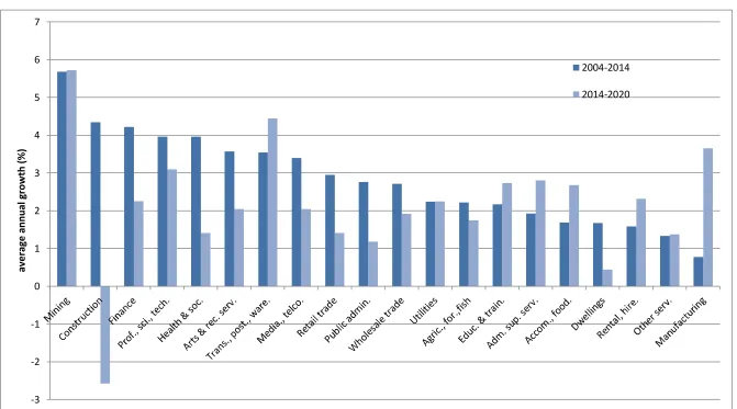
One of the concerns of Dog Days is that Australia’s recent experience of low productivity growth might continue over the short to medium term, leaving little to buoy growth in per capita real income if the terms of trade, mining investment and participation rate decline, as forecast (Garnaut 2013) (pp.130-139). The recent slow-down in Australia’s productivity growth has been documented in Parham (2012), together with an analysis of the industry-specific factors that help explain the economy-wide productivity outcome. Parham (2012) and Productivity Commission (2014) calculate multi-factor productivity (MFP) growth over eight productivity cycles spanning 1973/74 – 2012/13 (Figure 13). The annual average rate of MFP growth over this period was approximately 0.7 per cent. The period of peak productivity growth (at 2.5 per cent per annum) was 1993/94-98/99, reflecting the fruits of microeconomic reforms during the 1980s and 1990s (Parham, 2004). However, over the next three productivity cycles, annual average productivity growth declined, falling to 1.2 per cent over 1998/99-03/04, before falling again, to become negative over 2003/04-12/13. A number of authors have investigated the factors that have contributed to the recent fall in productivity growth, tracing somewhere between a quarter and three quarters of the slow-down to particular sectors and potential causal factors within these sectors.

The Productivity Commission (2009) notes that approximately 70 per cent of the sharp fall in Australian MFP growth over the period 2003/04-06/07 can be traced to contributions by three industries (mining, utilities, and agriculture) and that in each case transient factors played an

important role. These factors include lags between investment and output expansion (for mining), low rainfall leading to quantity restrictions on water demand and expensive investments in desalination and water treatment (for utilities), and drought (for agriculture).

(17)

Page | 11 to the annual level achieved between 2000 and 2008 (0.6 per cent). However, with perhaps another 0.15 percentage points of the slowdown potentially explained by overstatement of productivity growth in the 1990s (via exclusion of property and business services from the calculation of market sector productivity), Dolman notes that this still leaves approximately half a percentage point of annual productivity slowdown to be explained by other factors. Dolman suggests that part of the explanation might lie in the exceptional productivity performance of the 1990s, arising from once-off reforms in utilities, finance and communications. But some factors specific to the 2000s might also be important, such as the potential damping of incentives to find operational efficiencies during a period of

sustained high profitability, and the apparent general slowdown in productivity growth across developed countries, the latter suggesting the possibility of a more widespread reduction in the pace of innovation.

In explaining the productivity slowdown, Dolman excludes as important explanatory factors both changes in the level of education, and changes in spending on infrastructure, information and communication technology, and research and development. This might provide some comfort that Australia’s future rate of productivity growth has the potential to move back towards its historical average as the atypical structural pressures faced by the Australian economy in the 2000s recede (Parham 2012). Nevertheless, the latest productivity figures continue to disappoint, with Productivity Commission (2014) reporting a decline in multifactor productivity of -0.8 per cent per annum over 2011/12-12/13. Strong growth in capital inputs in mining, without commensurate output growth, was again an important factor. However, out of the twelve sectors comprising the market sector, only four (wholesale trade, retail trade, transport and postal, and financial and insurance services) recorded positive productivity growth (and then only at 0.1, 0.1, 0.0 and 0.4 per cent respectively).

On the basis of the Productivity Commission’s latest figures (PC 2014), Garnaut’s caution on the pace of productivity growth is well founded. However Parham (2012) also makes a good case that the “usual suspects” of lumpy investment / capital cycles, structural adjustment pressures, and drought might account for approximately three quarters of the measured productivity slowdown in the 2000s, leaving a relatively small role for policy-driven factors, and providing some scope for optimism regarding the future rate of productivity growth. In undertaking our forecast simulations, we must make a decision on the forecast rate of productivity growth. This decision will be important for our forecast outcomes for real wages and national income. Under an optimistic scenario, we might

(18)

Page | 12 2012/13. In formulating our MFP shock for the OA and DA scenarios, it is this figure that we

extrapolate into our forecast period. We assume that the rate of MFP growth outside of the mining and dwellings sectors is 0.3 per cent. For mining, we allow for endogenous movements in capital

productivity to accommodate exogenously determined BREE-consistent movements in forecast mining output. For installed dwellings capital, we assume a zero rate of MFP growth. With a zero rate of MFP growth in the dwellings sector, endogenous (but ultimately small) changes in mining

productivity, and 0.3% p.a. MFP growth in the rest of the economy, the economy-wide average rate of productivity growth over the forecast period is approximately 0.2% p.a. (row 10, Table 1).

4 SIMULATION RESULTS

4.1 The orderly adjustment (OA) scenario

We begin withFigure 1, which reports outcomes for demographic and labour market variables over both the historical period (2003/04 – 13/14) and the forecast period (2013/14 –19/20). As discussed in Section 3, under the OA scenario we assume that real wages adjust to maintain the employment rate at its 2013/14 level. Hence, with the employment rate given, total employment (hours) is governed by our assumptions relating to growth in the working age population, the participation rate, and hours worked per worker. As discussed in Section 3.7, the values we assign these variables follow ABS Series B (ABS, 2013c), and the 2010 IGR (Commonwealth of Australia, 2010). By 2019/20, the joint effect of these assumptions sees the forecast value for Australia’s population rising by 10.7 per cent relative to its 2013/14 value, while total employment (hours) rises by 9.8 per cent, leading to a 0.8 per cent fall in the ratio of employment to population. As reported in row 7 of Table 1, this represents a 0.13% p.a. annual gap in the population growth rate relative to the employment growth rate. This will be a contributing factor to our forecast for slow growth in a number of important per-capita measures of economic activity.

(19)

Page | 13 history). The slowdown in growth of capital inputs causes real GDP growth under the OA scenario to slow relative to recent history. Whereas real GDP growth in the ten years to 2014 averaged 2.92% p.a., under the OA scenario this slows to 2.09% p.a (Table 1, row 12). However growth in GDP is not constant over the forecast, with 2017-18 marking a significant slowdown in GDP growth. In the four years to 2018, real GDP grows at 2.4% p.a, however in the simulation’s final two years, the GDP growth rate slows to 1.5% p.a. As is apparent from Figure 2, growth in both labour and capital inputs are forecast to slow from 2018. Growth in capital inputs slows from a 2013-14 to 2017-18 average of 3.0% p.a. to an average for the two years following 2017-18 of only 1.6% p.a.. An important

contributing factor is growth in mining capital, which slows markedly from 2017/18 (Figure 5). Independently, growth in employment (hours) also falls significantly after 2017-18, falling from an average rate of 1.7% p.a. in the four years to 2017-18, to 1.3% p.a. in the final two years of the simulation. Here, the declining participation rate is the main factor, with 2018/19 marking the first year of large forecast decline. In the four years to 2017/18, the participation rate remains largely unchanged. However from 2018/19 onwards the participation rate is forecast to decline at 0.3% p.a. (Figure 1).

Figure 4 reports paths for real GDP, real (consumption price deflated) GNP, the components of real GNE and the terms of trade. All three components of real GNE (private and public consumption, and investment) are forecast to grow at rates slower than that of real GDP. For real private and public consumption, this reflects three aspects of our simulation. First, as reported in Figure 4 and discussed in Section 3, the terms of trade is forecast to fall to its 2005/06 level by 2019/20. We model nominal private consumption spending as a given proportion of household disposable income. Ceteris paribus, the decline in the terms of trade represents a fall in national income, and with it, household income, damping private consumption growth relative to real GDP growth. Second, as discussed in Section 3.6, we model those elements of federal fiscal consolidation related to tax increases and transfer payment reductions as a net increase in household direct taxation. This reduces household disposable income relative to what it would otherwise have been, adding a second damping influence on the forecast rate of growth in private consumption relative to real GDP. Third, our accounting for national income recognises that four-fifths of the capital stock of the mining sector is foreign owned. This damps forecast growth in GNP and household disposable income relative to GDP, and hence also damps private consumption growth relative to GDP. Public consumption is also forecast to grow at a rate slower than real GDP. As discussed in Section 3.6, this reflects forecast slow growth in public consumption spending as reported in the Economic Outlook accompanying the 2014 Commonwealth Government budget.

(20)

Page | 14 Together, these sources suggest a sharp decline in mining investment (Figure 5). For example, Barber

et al. (2014) see 2013 as the peak year of mining investment, forecasting a decline to less than half the 2013 level by 2017. Second, for a given level of employment and the capital stock, the forecast decline in the terms of trade causes capital construction costs to rise relative to capital rental rates, damping rates of return on capital.6 To ensure that long-run rates of return on capital do not fall below required rates of return, the rate of capital accumulation must decline relative to what it would

otherwise have been under a higher level for the terms of trade. Finally, as discussed in Section 3.4, we allow for a gradual rise in required rates of return over the forecast period, reflecting a gradual rise in interest rates as global monetary policy settings return to more normal settings.

Figure 6 reports paths for export and import volumes under the OA scenario. These paths show a strong movement towards balance of trade surplus over the forecast period, with export growth above, and import growth below, real GDP growth. As discussed in reference to Figure 4, growth in real GNE is forecast to be below growth in real GDP. The corollary of this is the strong move towards balance of trade surplus reported in Figure 6. The explanations for the movement towards balance of trade surplus thus mirror the explanations for why the path for real GNE lies below the path for real GDP: (i) the decline in the terms of trade, which necessitates a higher volume of exports to service a given volume of imports; (ii) significant foreign ownership of capital in the rapidly expanding mining sector, the repatriation of profits from which requires a movement towards balance of trade surplus; and, (iii) three forces acting to raise domestic savings relative to domestic investment: (a) damped growth in aggregate investment; (b) growth in public consumption below growth in real GDP; and (c) a rise in federal tax collections without commensurate spending growth, implying a rise in national saving relative to what it would otherwise have been. The resulting movement towards real balance of trade surplus requires real depreciation. In Figure 6, we see the required movement of the real

exchange rate over the forecast period is of the order of -20 per cent.

Figure 7 reports paths for selected per-capita measures of activity. Real GDP per capita rises between 2013/14 and 2017/18, but declines thereafter. For the first four years of the simulation period, 2013/14 to 2017/18, annual average real GDP growth is 2.4%, 0.7 percentage points per annum higher than the 1.7% p.a. population growth rate over the period. However, for the two years after 2018, the forecast for real annual average GDP growth, at 1.5%, is, on average, 0.1% lower than the annual average forecast for growth in the population, at 1.6% per annum. As discussed in reference to Figure 1, important contributors to the slowdown in post-2017/18 real GDP growth is a forecast decline in the

6

(21)

Page | 15 participation rate, damping employment growth, and the tapering of the mining project pipeline, which damps capital growth.

For measuring the incomes of Australians, real GNP, not real GDP, is the relevant measure. In Figure 7, we see that the path for per capita real GNP lies below the path for per capita real GDP. As

discussed in reference to Figure 4, the path for real GNP lies below that for real GDP because of the decline in the terms of trade and the allocation to foreign owners of a significant proportion of returns from new mining capital. Real GNP per capita is forecast to decline at an annual average rate of 0.31% (Table 1, row 22), representing not only an annual growth rate over half a percentage point below that forecast for real GDP per capita (Table 1, row 21), but also a significant slowdown on the previous decade’s average per capita GNP growth rate of 1.66% p.a (Table 1, row 21). The forecast average growth in real GNP per capita of -0.31% p.a. again obscures 2017/18 as an important turning point, with the growth rate in the four years to 2017/18 averaging -0.1% p.a., but with this declining to -0.7% p.a. over the subsequent two years (Figure 7). Forecast growth rates for real consumption per capita are also negative. For real private consumption, which is forecast to grow at -0.85% p.a., this reflects the joint effect of the decline in real GNP, which depresses household pre-tax incomes, and the rise in federal net direct taxation, which depresses household post-tax incomes. The outcome for per capita public consumption, which is forecast to grow at -0.6% p.a., reflects our forecast for slow growth in aggregate public consumption spending.

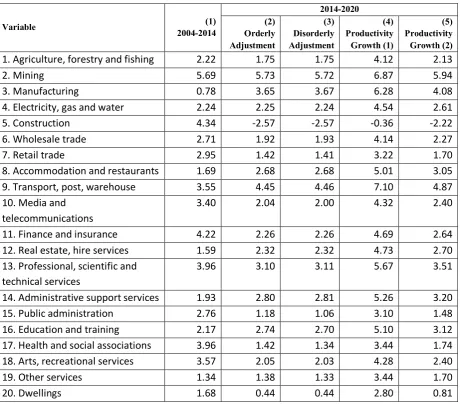
While VIC-UNI models activity for 106 industries, for reporting purposes we aggregate outcomes for output by industry to the 20 broad sectors, reported in Figure 8 and Table 2. Mining is projected to experience the largest output expansion over the forecast period (5.7% p.a., row 2, Table 2). This reflects the strong growth in mining output forecast by BREE (2014). The transport sector is projected to be the second-fastest growing sector over the simulation period. While not reported in Figure 8 or Table 2, three transport sub-sectors - rail and water transport, and transport services - are projected to benefit from the provision of margin services to mining exports. A fourth transport sector, air

(22)

Page | 16 While output growth for trade-exposed sectors is favourable, domestically-oriented sectors are

projected to experience poor growth prospects, relative to GDP, over the forecast period. The sector with the lowest growth prospects is construction, reflecting the high proportion of its activity that is explained by sales to investment. As explained with reference to Figure 5, the end of the mining boom, together with the decline in the terms of trade and projected rise in required rates of return, sees

aggregate investment decline over the simulation period. This same pattern of decline is reflected in the path for construction output, which peaks in 2013, before declining to levels reminiscent of 2005/06 by 2018/19 (Figure 8). Comparing columns (1) and (2) of Table 2, we see that this translates into the largest fall in growth experienced by any sector. In annual average terms, construction output growth declines from its decade average rate of 4.3% p.a. to -2.5% p.a. (row 5, Table 2). Other slow-growing sectors are exposed to the forecast slow growth for private and public consumption. These sectors include retail trade, other services, dwellings, public administration, health and social associations, and arts and recreational services.

4.2 The disorderly adjustment (DA) scenario

(23)

Page | 17 of approximately 2.7%, after which it tracks below the OA wage path. Despite the near return of the employment rate to its OA level by 2019/20, the real wage remains approximately 0.2% below its 2019/20 OA level (Figure 9). This reflects a decline in the terms of trade under the DA scenario relative to the OA scenario, as the balance of trade is required to move towards surplus, relative to the OA scenario, to return the net foreign debt / GDP ratio to its OA scenario level (see Figure 12).

Figure 10 reports DA outcomes for real GDP, the capital stock, and employment, comparing these with outcomes under the OA scenario. The decline in the employment rate relative to that under the OA scenario (Figure 9) causes employment (hours) to initially lie below its OA value, before

gradually moving back towards its OA value (Figure 10). Despite the eventual return of employment to its OA level, it is clear from Figure 10 that DA employment lies below OA employment for much of the simulation period. One summary measure of the labour market disruption generated under DA is to convert the area between the OA and DA employment paths into lost annual jobs. Beginning with a figure for average 2013/14 employed persons of 11.5 m. (ABS 2014j), the employment growth paths for persons under the OA and DA scenarios imply lost job-years of the order of 250 thousand persons.

The aggregate capital stock under the DA scenario closely tracks the capital stock under the OA scenario. For the first two years of DA, aggregate investment is subject to two countervailing forces: (i) the decline in employment, relative to OA, depresses the marginal product of capital, damping investment relative to OA; (ii) the rise in consumption spending, relative to OA, causes the balance of trade to move towards deficit relative to OA, increasing the terms of trade, and thus raising the rate of return on capital, and with it, investment, relative to OA. We see this in Figure 11, where aggregate DA investment closely tracks aggregate OA investment over the simulation’s first two years. In 2016/17, aggregate investment under DA falls 1% below its OA value (Figure 11), reflecting the sharp decline in real consumption spending in that year (Figure 11) at a time when employment remains below its baseline value (Figure 10).

Returning to Figure 10, with the DA scenario capital stock tracking closely its OA level, but with DA scenario employment lying below its OA level, real GDP under the DA scenario lies below its OA value. Real GDP has nearly returned to its OA value by the end of the simulation period, reflecting the return of employment to its OA value. Hence, in columns 2 and 3 of Table 1, we see little difference in the annual average real GDP growth rates under the two scenarios (row 12).

(24)

Page | 18 simulation’s first two years (Figure 12). Thereafter, we assume that real consumption follows a path that steadily returns the net foreign debt / GDP ratio to its OA value.7

Figure 12 reports per-capita outcomes for real GDP, real GNP and real aggregate consumption per capita, comparing OA and DA outcomes for each. After two years of maintenance of real per capita consumption, the assumption that consumption is then placed on a path from 2016/17 that returns the net foreign debt / GDP ratio to its OA level requires an initial steep fall in 2016/17 consumption, of the order of 4.4%. This fall can be viewed as comprising two parts: a 2.5% fall to bring DA

consumption to its 2016/17 OA level, and a further 1.9 percentage points of reduction to lower DA consumption further, below its OA level, in order to generate the savings required to steadily return the net foreign debt / GDP ratio back to its OA level.

By the end of the simulation period, real GDP per-capita has returned to close its OA level (Figure 12). However, this is not the case for either per capita real GNP or per capita real consumption, both of which remain below their OA levels in 2019/20. For real GNP per-capita, this reflects two things. First, the initial increase in real consumption carries with it a rise in net foreign liabilities relative to the OA scenario. Much, but not all, of the 2014/15-15/16 increase in net foreign liabilities relative to OA has been eliminated by 2019/20 through the sharp post-2015/16 cut in consumption spending (Figure 12, right hand axis). The fact that not of all the additional net foreign debt incurred over 2014/15-15/16 has been repaid by 2019/20 depresses the outcome for DA real GNP relative to its 2019/20 OA value. With the 2019/20 DA value for real GNP per capita lying below its OA value, we would expect the 2019/20 DA value for real consumption per capita to also lie below its OA value. As we see in Figure 12, this is the case, however the gap between 2019/20 values for real per capita consumption under the OA and DA scenarios exceeds the gap in 2019/20 real GNP outcomes. This reflects our assumption of gradual return of the net foreign debt / GDP ratio to its OA level. By 2019/20, this process is not complete, requiring consumption to remain depressed relative to its OA level at the end of the simulation period, to continue generating the savings required to return the net foreign debt / GDP ratio to its OA level.

4.3 The productivity growth scenarios (PG1 and PG2)

Dog Days discusses a number of the possible policies that might be implemented in response to the challenges posed by the mining boom’s end, covering four policies that we might broadly describe as

7

(25)

Page | 19 macroeconomic (“business-as-usual”,” austerity”, “stimulus” and “real depreciation”) and one that we might broadly describe as microeconomic (productivity growth). Our modelling of the OA and DA scenarios cover a number of the macroeconomic policy dimensions discussed by Garnaut. Certain elements of the responses described as “business-as-usual” and “stimulus”, particularly as they relate to a failure to calibrate consumption growth to the new realities of national income in the post-boom environment, are modelled within our DA scenario. Second, with respect to “real depreciation”, our OA scenario projects endogenous real depreciation of the order of 20% between 2013/14 and 2019/20 (Figure 6). A fall in the real exchange rate of this magnitude would place it near the centre of the range of real depreciation outcomes that Garnaut anticipates will be required to accommodate the end of the mining boom.8 As such, our OA scenario can be viewed as incorporating a key element of the “real depreciation” policy response. Of the five policies, Garnaut rightly notes that only productivity growth can permanently raise living standards, making policy to lift productivity the appropriate response to the permanent decline in living standards that will follow from the terms of trade returning to, and thereafter remaining at, its 2005/06 level. In this section, we focus on productivity, exploring the magnitude of the increase in multifactor productivity growth that will be required to sustain living standards across the otherwise adverse economic environment described by our Orderly Adjustment (OA) scenario.

Under our OA scenario, real (consumption price deflated) GNP per capita is forecast to decline at an annual average rate of 0.31% over 2013/14-2019/20, a decline of almost two percentage points on the annual average achieved over the decade 2003/4-13/14 (Table 1, row 22). As discussed in Section 4.1, the fall in the growth rate of real GNP per capita is attributable in large part to the forecast decline in the terms of trade (row 8). Relative to recent history, MFP growth under the OA scenario is forecast to add 0.20 percentage points to annual real GDP growth (row 10). While this is an improvement on the period 2003/4-2013/14, as discussed in Section 3.8, it is nevertheless low by historical standards. In the first of our productivity growth scenarios (PG1), we ask the model to answer the following question: what rate of MFP growth will be required to allow real GNP per capita to grow over 2013/14-19/20 at an annual average rate equal to that achieved over 2003/4-13/14, i.e. 1.66%? To calculate this, we run a simulation that is identical to the OA scenario in all respects except:

(i) We exogenously determine growth in real GNP per capita at 1.66% p.a., and endogenously determine economy-wide primary factor productivity growth.

8

(26)

Page | 20 (ii) We exogenously determine the ratio of public to private consumption spending at its OA

level in each year of the simulation period, while endogenously determining real public consumption spending. With private consumption spending determined via a fixed propensity to consume out of household disposable income, this indexing of public to private consumption allows both public and private consumption to follow a higher path under the PG scenario relative to the OA scenario, consistent with the higher level of national income under PG relative to OA.

As reported in row 10 of Table 1, to achieve forecast annual growth in real GNP per capita of 1.66 % p.a., productivity growth must rise from its OA forecast value of 0.2%p.a. to 1.96%p.a.Because these figures exclude contributions to output growth from the emergence of lagged mining investment, official MFP growth, as reported by the ABS, will need to be higher. Row 9 of Table 1 reports MFP calculated on the ABS basis of crediting capital’s contribution to output in the period following investment, rather than in the period in which the capital becomes functional (the latter being the basis for the MFP calculation reported in row 10). Comparing rows 9 and 10, we see that official MFP growth over the forecast period contains approximately 0.2% p.a. of GDP contribution more properly attributed to lagged capital supply, than to efficiency improvement.

To put the required productivity improvement in context, Figure 13 compares this with four decades of productivity growth as reported in Parham (2012) and Productivity Commission (2014).9 As is clear from Figure 13, Australia’s peak period of productivity growth was 1993/94-98/99 (at 2.5 per cent per annum), although the productivity growth rate remained high over the following four years to 2003/04 (at 1.2 per cent per annum), before falling below zero over the period 2003/04 – 12/13. The magnitude of the productivity challenge that Australia faces in maintaining recent growth in living standards is clear when we see that, while not unprecedented, productivity growth in the vicinity of 2.0% p.a. has not occurred since the mid-1990s, and only then, following a period of policy resolve at both state and federal levels to engage in significant structural reform. In the absence of a recent history of such reform, and in the context of the past decade’s experience of low or negative productivity growth, the sudden re-emergence of productivity growth in the vicinity of 2.0% p.a. is not plausible. Given this, we might instead ask, what level of productivity growth will be required to maintain living standards over the forecast period? Our second productivity growth scenario (PG2) investigates this question. PG2 is like PG1 in all respects except that, instead of exogenously determining growth in real GNP per capita at 1.66% p.a., we instead hold real GNP per capita constant over the simulation period (Table 1, row 22, column 5). Consistent with this being a less ambitious real GNP target than that set in PG1, the required growth in productivity is commensurately

9

(27)

Page | 21 modest, at 0.49% p.a. (Table 1, row 10, column 5). Looked at in the historical context portrayed in Figure 13, the PG2 scenario’s MFP growth of 0.49% looks a plausible if ambitious target, one that might prove feasible within the context of a concerted policy effort to raise MFP through a

comprehensive program of microeconomic reform, but one that might also prove unattainable, particularly if the reform complacency described in Dog Days is to continue.

5 Concluding Remarks

Since the end of the recession of the early 1990s, Australia has enjoyed a long period of uninterrupted economic growth. Growth in real income has been particularly strong over the past decade, with real GNP per capita rising at an annual average rate of over 1.6 per cent. However, as Garnaut (2013) warns, a careful analysis of prudent forecasts for the factors that have lain behind the recent history of strong income growth – particularly growth in the terms of trade and in mining investment – suggests that Australia will soon face challenges in maintaining its recent history of rising real income.

In this paper, we have used an economy-wide model, VIC-UNI, to generate a forecast for the

Australian economy to 2019/20. For inputs to the model, we have relied both on independent forecasts for the terms of trade, mining investment, mining output, mining export prices, demographic and labour market variables, public expenditures and direct taxation, and on our own plausible assumptions about paths for required rates of return, post-tax foreign ownership claims on capital returns, and growth in multifactor productivity. Without explicitly setting out to do so, the forecast that we generate in this way replicates salient features of the pessimistic picture for the immediate future of the Australian economy depicted in Dog Days.

Key elements of our input assumptions, particularly as they relate to our forecast for per capita national income, are: a return of the terms of the trade to its 2005/06 level by 2019/20, a halving in mining investment from its peak 2012/13 level by 2019/20, a gap between the forecast annual growth rates for population and employment, and a high rate of foreign ownership of the mining sector. But not all of our input assumptions are pessimistic. In forming a view on future multifactor productivity growth, we assume a continuation of the 0.3% p.a. rate of productivity growth experienced by the non-mining market sector over 2003/04 – 2012/13. Excluding the housing stock from this

(28)

Page | 22 With these assumptions in place under our orderly adjustment scenario, we forecast aggregate real GDP growth of approximately 2.1% p.a. This is only a little higher than the ABS Series B annual average population growth rate over the period, leaving real GDP per capita rising by just under 0.4% p.a.. However, the forecast decline in the terms of trade, and the high level of foreign ownership of the rapidly expanding mining sector, together damp forecast real GNP growth relative to real GDP growth. With little growth forecast for real GDP per capita, this leaves our forecast for real GNP per capita negative, at approximately -0.3% per annum. With forecasts for slow growth in public consumption spending and a rise in direct taxation, our forecast for annual average growth in per-capita real consumption spending is lower still, at -0.8%. With growth rates in these ranges, we forecast under our orderly scenario that important measures of economic welfare, such as the real wage, real GNP per capita, and real consumption per-capita, will return to the levels of the late-2000s by the end of the decade.

However as Garnaut (2013) notes, there are risks of mismanagement of the policy adjustments that will be required in the face of Australia’s new economic realities. We simulate this in a disorderly adjustment scenario, one in which we assume that the private and public sectors initially attempt to maintain current consumption and wage levels, despite slower growth in national income. For two years we hold real per-capita public and private consumption, and the real consumer wage, unchanged at their 2013/14 levels. Relative to the orderly adjustment scenario, this generates rising net foreign debt and unemployment. In the simulation’s third year, we put wages and savings on paths that gradually return net foreign debt and the unemployment rate to their levels under the orderly adjustment scenario. The macroeconomic adjustments that this scenario entails generate significant volatility in consumption, unemployment rates, wage rates, and net foreign debt, while ultimately placing the economy in a 2019/20 position that is little different to that attained under the orderly adjustment scenario. However, with employment below its orderly adjustment path for much of the disorderly scenario, the lost potential employment is equivalent to approximately 250 thousand one-year jobs over the period 2013/14 – 2019/20.

The maintenance of our recent experience of rapid growth in per-capita income will require a rate of multifactor productivity growth that exceeds the 0.2% p.a. of our orderly adjustment scenario. In our final two simulations, we ask the model to uncover the rates of multifactor productivity growth that will be required to either: (i) maintain the decade average growth rate in real GNP per capita of just over 1.6% p.a.; or (ii) simply maintain real GNP per capita unchanged through to 2019/20 at its 2013/14 level. Achievement of the first target, maintenance of our recent experience of rapid per-capita real GNP growth, will require multifactor productivity growth to rise to approximately 2.0% p.a., a rate not seen since the mid-90s. Achievement of the more modest second target, maintenance of the 2013/14 level of real per capita GNP, still requires a significant increase in multifactor

(29)

Page | 23 over 1973/74 to 2012/13, but higher than rates achieved over the last decade. The official ABS

headline rates of productivity growth will need to be higher still. Because our model allows for lags between mining investment and mining capital supply, our forecasts for multifactor productivity growth are not affected by lags between mining investment and output, as are the ABS rates. Over our forecast period, the effect of mining output coming on stream as a result of investment booked by the ABS as functional capital in its calculation of the MFP growth of earlier periods will lead reported ABS MFP growth to exceed our MFP growth rate by approximately 0.2% pa. Hence, in interpreting future MFP headlines, this portion of reported productivity growth will need to be recognised as a

timing matter, and not a true representation of the nation’s underlying productivity performance.

(30)

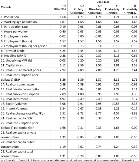
Page | 24 Table 1: Summary comparison: forecast simulation results (2014-2020) vs recent history (2004-2014) (Average annual growth rates, per cent)

Variable (1) 2004-2014 2014-2020 (2) Orderly Adjustment (3) Disorderly Adjustment (4) Productivity Growth (1) (5) Productivity Growth (2)

1. Population 1.68 1.71 1.71 1.71 1.71

2. Working age population 1.81 1.68 1.68 1.68 1.68

3. Participation rate 0.19 -0.06 -0.06 -0.06 -0.06

4. Hours per worker -0.40 -0.05 -0.05 -0.05 -0.05

5. Employment rate -0.02 0.00 -0.01 0.00 0.00

6. Employment (hours) 1.57 1.57 1.56 1.57 1.57

7. Employment (hours) per person -0.10 -0.13 -0.14 -0.13 -0.13

8. Terms of Trade 4.25 -3.44 -3.48 -4.15 -3.56

9. Headline MFP (a) -0.28 0.37 0.37 2.13 0.66

10. Underlying MFP (b) -0.03 0.20 0.20 1.96 0.49

11. Capital stock 5.12 2.56 2.55 2.81 2.58

12. Real GDP at market prices 2.92 2.09 2.08 4.29 2.44

13. Real (consumption price

deflated) GNP 3.36 1.39 1.37 3.39 1.71

14. Real consumer wage 0.89 -0.89 -0.92 0.87 -0.62

15. Real private consumption 3.05 0.84 0.83 2.72 1.14

16. Real public consumption 2.89 1.08 0.95 2.96 1.38

17. Real Investment 4.97 -2.49 -2.49 -0.49 -2.17

18. Export Volumes 3.96 7.91 7.95 10.53 8.35

19. Import Volumes 6.34 0.67 -0.38 1.21 -0.12

20. Real exchange rate (PGDP/PM) 2.51 -3.73 -3.77 -4.57 -3.88

21. Real per capita GDP 1.22 0.38 0.37 2.54 0.73

22. Real (consumption price

deflated) per capita GNP 1.66 -0.31 -0.33 1.66 0.00

23. Real per capita private

consumption 1.35 -0.85 -0.86 1.00 -0.56

24. Real per capita public

consumption 1.19 -0.61 -0.74 1.24 -0.32

25. Real per capita total

consumption 1.31 -0.79 -0.83 1.05 -0.50

(a) June 04 – June 13, Market sector multifactor productivity, perpetual inventory method. Negative denotes productivity decline. (ABS 5204.0, 2012-13). In row 9, for calculating MFP over the forecast period, we follow the ABS method of assuming capital services are available immediately after investment. Hence, the forecast MFP figure in row 9 includes capital service returns from lagged investment.

(31)

(32)

Page | 26 Table 2: Output by sector: forecast simulation results (2014-2020) and recent history (2004-2014) (Average annual growth rates, per cent)

Variable (1) 2004-2014 2014-2020 (2) Orderly Adjustment (3) Disorderly Adjustment (4) Productivity Growth (1) (5) Productivity Growth (2) 1. Agriculture, forestry and fishing 2.22 1.75 1.75 4.12 2.13

2. Mining 5.69 5.73 5.72 6.87 5.94

3. Manufacturing 0.78 3.65 3.67 6.28 4.08

4. Electricity, gas and water 2.24 2.25 2.24 4.54 2.61

5. Construction 4.34 -2.57 -2.57 -0.36 -2.22

6. Wholesale trade 2.71 1.92 1.93 4.14 2.27

7. Retail trade 2.95 1.42 1.41 3.22 1.70

8. Accommodation and restaurants 1.69 2.68 2.68 5.01 3.05

9. Transport, post, warehouse 3.55 4.45 4.46 7.10 4.87

10. Media and telecommunications

3.40 2.04 2.00 4.32 2.40

11. Finance and insurance 4.22 2.26 2.26 4.69 2.64

12. Real estate, hire services 1.59 2.32 2.32 4.73 2.70

13. Professional, scientific and technical services

3.96 3.10 3.11 5.67 3.51

14. Administrative support services 1.93 2.80 2.81 5.26 3.20

15. Public administration 2.76 1.18 1.06 3.10 1.48

16. Education and training 2.17 2.74 2.70 5.10 3.12

17. Health and social associations 3.96 1.42 1.34 3.44 1.74

18. Arts, recreational services 3.57 2.05 2.03 4.28 2.40

19. Other services 1.34 1.38 1.33 3.44 1.70

(33)

Page | 27

Figure 1: OA Scenario: Demographic and labour market variables (levels, 2014 base = 1)

0.825

0.875 0.925 0.975 1.025 1.075 1.125

2004 2005 2006 2007 2008 2009 2010 2011 2012 2013 2014 2015 2016 2017 2018 2019 2020

Participation rate

Population (aged 15+)

Population (total)

Employment (hours)

Employment rate

Hours per person (population) Hours per worker

(34)

Page | 28

Figure 2: OA Scenario: Employment, capital stock, MFP contribution to real GDP (levels, 2014 base = 1)

0.6 0.7 0.8 0.9 1 1.1 1.2

2004 2005 2006 2007 2008 2009 2010 2011 2012 2013 2014 2015 2016 2017 2018 2019 2020

Real GDP

Capital

Contribution of productivity

(35)

Page | 29

Figure 3: Contribution of depreciation deductions to post-tax foreign capital returns, expressed as a percentage of GDP

0.6 0.65 0.7 0.75 0.8 0.85 0.9

(36)

Page | 30

Figure 4: OA Scenario: Real GDP, real GNP, the components of real GNE, and the terms of trade (levels, 2014 base = 1)

0.6 0.7 0.8 0.9 1 1.1 1.2

2004 2005 2006 2007 2008 2009 2010 2011 2012 2013 2014 2015 2016 2017 2018 2019 2020

Real Private Consumption

Real Public Consumption

Real Investment

Terms of Trade

Real GDP

(37)

Page | 31

Figure 5: Forecast mining investment, capital stock and output (levels, 2014 base = 1)

0.4 0.6 0.8 1 1.2 1.4 1.6

2004 2005 2006 2007 2008 2009 2010 2011 2012 2013 2014 2015 2016 2017 2018 2019 2020

(38)

Page | 32

Figure 6: OA Scenario: Export volumes, import volumes, real exchange rate measures (levels, 2014 base = 1)

0.4 0.6 0.8 1 1.2 1.4 1.6 1.8

2004 2005 2006 2007 2008 2009 2010 2011 2012 2013 2014 2015 2016 2017 2018 2019 2020

Export Volumes Import Volumes Real GDP

(39)

Page | 33

Figure 7: OA Scenario: Per-capita measures of economic activity (levels, 2014 base = 1)

0.8 0.85 0.9 0.95 1 1.05

2004 2005 2006 2007 2008 2009 2010 2011 2012 2013 2014 2015 2016 2017 2018 2019 2020

Real aggregate consumption, per capita

Real private consumption, per capita

Real public consumption, per capita

Real GNP per capita

(40)

Page | 34

Figure 8: OA Scenario: Average annual growth in output per industry

-3 -2 -1 0 1 2 3 4 5 6 7

average annual growth (%)

(41)

Page | 35

Figure 9: DA Scenario: Employment rate and the real consumer wage (levels, 2014 base = 1)

0.94 0.95 0.96 0.97 0.98 0.99 1 1.01 1.02

2012 2013 2014 2015 2016 2017 2018 2019 2020

Employment rate (OA)

Real consumer wage (OA)

Employment rate (DA)

(42)

Page | 36

Figure 10: DA Scenario: Employment, capital and real GDP (levels, 2014 base = 1)

0.9 0.95 1 1.05 1.1 1.15 1.2

2012 2013 2014 2015 2016 2017 2018 2019 2020

Employment (hours) (DA)

Real GDP (DA)

Capital Stock (DA)

Capital Stock (OA)

Real GDP (OA)

(43)

Page | 37

Figure 11: DA Scenario: Real GDP and the components of real GNE (levels, 2014 base = 1)

0.8 0.85 0.9 0.95 1 1.05 1.1 1.15

2012 2013 2014 2015 2016 2017 2018 2019 2020

Real GDP (DA)

Real Private Consumption (DA) Real Public Consumption (DA) Real Investment (DA)

Real GDP (OA)

(44)

Page | 38

Figure 12: DA Scenario: Per-capita measures of economic activity (levels, 2014 base = 1)

0 0.002 0.004 0.006 0.008 0.01 0.012

0.95 0.96 0.97 0.98 0.99 1 1.01 1.02 1.03

2012 2013 2014 2015 2016 2017 2018 2019 2020

Real aggregate consumption, per capita

Real GNP per capita

Real GDP per capita

Real aggregate consumption, per capita (OA)

Real GNP per capita (OA)

Real GDP per capita (OA)

(45)

Page | 39

Figure 13: Australian multifactor productivity, annual growth rates.

Sources: Figure 1.1 reproduced from Parham (2012), updated with 2003/04-07/08 and 2007/08-12/13 values Productivity Commission (2014)

Quantifying "Dog Days"

Centre of Policy Studies Working Paper

No. G-246 July 2014