Object Classification in Still Images
T.Harini
1, J.Uday Kiran
2, Prof. P.Pradeep
1, K. Jhansi Rani
3 1CSE, Vivekananda Institute of Technology and Science, Karimnagar, AP, India2Indian Institute of Science, Bangalore, Karnataka, India
3ECE, Vivekananda Institute of Technology and Science, Karimnagar, A.P, India
Abstract-The goal of the Object Classification is to classify the
objects in images. Classification aims for the recognition of generic classes, which is also known as Generic Object Recognition. This is quite different from Specific Object Recognition, such as recognizing specific person, own car, and etc. Human beings are generally better in recognizing generic classes than specific objects. Classification is a much harder problem to solve by artificial systems. Classification algorithm must be robust to changes in illumination, object scale, view point, and etc. The algorithm also has to manage large intra class variations and small inter class variations. In recent literature, some of the classification methods use Bag of Visual Words model. In this work the main emphasis is on region descriptor and representation of training images. Given a set of training images, interest points are detected through interest point detectors. Region around an interest point is described by a descriptor. Region covariance descriptor is adopted from porikli et al. [21], where they used this descriptor for object detection and classification. This region covariance descriptor is combined with Bag of Visual words model. We have used a different set of features for Classification task. Covariance of d-features, e.g. spatial location, Gaussian kernel with three different s values, first order Gaussian derivatives with two different s values, and second order Gaussian derivatives with four different s values, characterizes a region of interest. An image is also represented by Bag of Visual words obtained with both SIFT and Covariance descriptors. We worked on five datasets; Caltech-4, Caltech-3, Animal, Caltech-10, and Flower (17 classes) [25], with first four taken from Caltech-256
[24] and Caltech-101 [23] datasets. Many researchers used Caltech-4 dataset for object classification task. The region covariance descriptor is outperforming SIFT descriptor on both Caltech-4 and Caltech-3 datasets, whereas Combined representation (SIFT +
Covariance) is outperforming both SIFT and Covariance
Keywords: Object recognition, Object classification, Bag of visual words, region covariance descriptor, SIFT descriptor
I. INTRODUCTION
Object Classification is the process of classifying images based on the objects that are in the images. A two class classifier classifies each object as either class object or non-class object. The non-classifiers are trained with a certain training dataset. The images in each category consist of objects with varying scales, different illuminations, and different view-points. The algorithm must be robust to changes in view point, scale, and illumination. This algorithm can also be used to categorize objects from dynamic scenes. Objects can be extracted from the dynamic scene by video object segmentation. In ideal case, intra class variance must be low and inter-class variance must be high.
But in practice intra-class variance is high and inter-class variance is low.
A. Problem
Object classification is defined as the process of assigning an object to a category. This is also known as Generic Object Recognition. This Generic Object Recognition is different from the Specific Object Recognition. In Generic Object Recognition, the objects like people, cars, trees, flowers are classified, where as in Specific Object Recognition, the objects like a specific person, your own car are classified. Humans are better at categorizing the objects, whereas the artificial systems are better at Specific Object Recognition.
B. Motivation
Object recognition by computer has been an active area of research for nearly five decades. For much of the time, the approach has been dominated by the discovery of analytic representations (models) of objects that can be used to predict the appearance of an object under any viewpoint and under any conditions of illumination and partial occlusion. The expectation is that ultimately a representation will be discovered that can model the appearance of broad object categories and in accordance with the human conceptual framework so that the computer can tell what it is seeing. There are a number of reasons why geometry has played such a central role like Invariance to viewpoint, illumination, well developed theory, manmade objects. Current state of object recognition research is that, the four decade dependence on step edge detection for the construction of object features has been broken. Step edge boundaries are still useful in forming an object description where the object surface is clutter free. But, for a large fraction of object surfaces and textures, affine patch features can be reliably detected without having to confront the difficult perceptual grouping problems that are required to form purely geometric boundary descriptions from edges. Current research focuses on data driven, machine learning, appearance based models. The following are some of the issues involved.
Robustness with respect to variation in viewpoint, illumination, scale and imaging conditions.
Scaling up to hundreds of object classes. While some applications may only require class libraries of dozens of objects, many require much larger class diversity requiring human-level performance.
C. Applications
pedestrians, Warning of exit advance track, Detection of driver’s sleepiness
Computational photography - Computational photography refers broadly to computational imaging techniques that enhance or extend the capabilities of digital photography. The output of these techniques is an ordinary photograph, but one that could not have been taken by a traditional camera. Visual understanding of a given image/scene has following applications in computational photography like Photo Tourism; Exploring photo collections; face detection
Content based image retrieval - Content-based indexing via automatic object detection and recognition techniques has become one of most important and challenging issues for the years to come, in order to face the limitation of traditional information systems. Some of the expected applications are: Information and entertainment video production and distribution, Professional video archive management including legacy footage, Teaching, training, enterprise or institutional communication, TV program monitoring, Self-produced content management, Internet search engines (Visual Search), Advanced object-based image coding.
II. OBJECT CLASSIFICATION
Object Classification task is divided into five sub-problems. Every sub-problem is explained in detail in following sections. The algorithm used in this work follows the following steps.
• Interest Point detection • Feature extraction
• Visual Vocabulary Generation and Bag of Visual words • Learning classifiers
Interest point detectors are used to get interest points in the given images. Interest point detectors available in the literature are discussed in the following sections. Once the interest points are available, features can be extracted from a region around each interest point and size of the region of interest is dependent on scale of the interest point. The descriptors or feature extractors available in the literature are given in the following sections. Once a set of feature vectors extracted from training images are available, each and every feature need not be used to train the classifier. One more important point to be observed is, number of interest points in any two images might not be same. Therefore the number of feature vectors of any two images might not be same. But the current machine learning algorithms require images to be represented by same number of feature vectors. Here comes the concept of Bag of Visual Words. Feature vectors extracted around interest points are grouped into a large number of clusters. The regions with similar descriptors are assigned into the same cluster. Here each cluster is treated as “visual word”. Each “visual word” represents the specific local pattern shared by the regions in that clusters. Visual Vocabulary represents such local pattern in the given set of training images. By mapping region descriptors of an image into visual words, an image can be represented as a “bag of visual of words” or specifically, as a vector containing the
count of each visual word in that image, which is further normalized and used as feature vector of an image in the training and classification task. The next task is to train a classifier for each category. The process of training is supervised, since the labels of the images are known. Each classifier is trained with a certain set of positive and negative examples. The training algorithms in literature are broadly categorized into Discriminative models and Generative models.
A. Interest Point Detectors
A local feature is an image pattern which differs from its immediate neighborhood. Local features can be points, but also edges or small image patches. Some measurements are taken from a region centered on a local feature and converted into descriptors. Local features can be broadly categorized into three categories based on possible usage.
• Those have specific semantic interpretation in the limited context of a certain application.
• Those provide a limited set of well localized and individually identifiable anchor points.
• Can be used as a robust image representation that allows recognizing objects or scenes without the need for segmentation. The various detectors available in literature are Corner detectors (Harris, SUSAN detectors, Harris-Laplace, Harris-Affine) and Blob detectors (Hessian, Hessian-Laplace/Affine detectors) and Region detectors (Intensity based regions, maximally stable extremal, segmentation based methods).
SIFT features are invariant to scale and rotation and it is 128 dimensional vector. Given the interest point and scale, a patch is considered around the interest point. The patch is divided into 4 *4 cells. A histogram of eight orientations is obtained for each cell. Each bin is weighted by the magnitude of gradient of the pixel. This results in 128-dimensional descriptor. A new descriptor is used instead of SIFT, which is as explained below.
1) Covariance Descriptor
The covariance of d features characterizes a region of interest. Features like three-dimensional color vector, the norm of first and second derivatives of intensity with respect to x and y are used. The region of interest can be represented by Covariance of the feature vectors’. The covariance matrices are low dimensional compared to other region descriptors and the number of different elements is only (d2+d)/2 due to symmetry of Covariance matrix CR. In this
F
(x,y
)=
(R,x,y) where R is the region of interest, s is the dimension of the patch’s side which is directly proportional to the scale of the interest point, and the function - can be any mapping such as intensity, color, gradients, filter responses, etc. For the region of interest R, let {zk}k=1::n be the ddimensional feature points inside R. The region of interest R can be represented with a d*d covariance matrix of the feature points
CR
=
n(z
k-
)(zk-
)
T/(n-
1)
where is the mean of the points in the region of interest. There are several advantages of using covariance of feature points as region descriptor. A single covariance extracted from a region is generally enough to match with different views and poses of the region. The covariance descriptor also provides
a way to fuse the different features which might be correlated. The diagonal elements of the covariance matrix are variances of the features and the off-diagonal elements are correlations between features.
B. Feature Extraction
Local interest points in an image can be obtained by interest point detectors. Interest point detectors give the location and scale of all interest points in the image. Given the interest point location and scale a patch around the interest point is taken. A feature vector is extracted from the patch, which represents the patch or region of interest.
1) Scale Invariant Feature Transform
Scale Invariant Feature Transform is proposed by D.G.Lowe [19]. It combines scale invariant region detector and a descriptor based on the distribution of gradients in the regions detected by scale invariant region detector. The detected region in gradient image is divided into 4 * 4 grids. The descriptor is represented by a 3-D histogram of locations and orientations. The contribution to the bin is weighted by gradient magnitude. The gradient angle is quantized into 8 orientations. There are 16 small regions in the detected region. The descriptor is 128-dimensional vector.
C. Visual Vocabulary Generation
The visual vocabulary represents the local patterns in the given set of training images. Each image is represented as a histogram and each bin of the histogram corresponds to a visual word taken from visual vocabulary formed. K-means and GMMs clustering techniques are used to form
vocabulary.
1) K-means Clustering
Given a set of feature vectors {x1; x2; x3; ::::; xn}, where each feature is a d-dimensional real vector, then K-means clustering aims to partition this set into K partitions S = S1; S2; S3; ::::; Sk so as to minimize the within-cluster sum of square errors. A feature vector is assigned to a cluster whose center is closer.
D. Learning Classifiers
As mentioned earlier there are two different models, generative and discriminative. All algorithms fit in to one of the above mentioned models. Consider a scenario in which an image is described by a vector W (which might comprise raw pixel intensities, or some set of features extracted from the image) is to be assigned to one of Z classes {z = 1, . . .,Z}.
From basic decision theory we know that the most complete characterization of the solution is expressed in terms of the set of posterior probabilities P(z|W). Once we know these probabilities it is straightforward to assign the image to a particular class to minimize the expected loss (for instance, if we wish to minimize the number of misclassifications we assign image to the class having the largest posterior probability).
In a discriminative approach we introduce a parametric model for the posterior probabilities, P(z|W), and infer the values of the parameters from a set of labeled training data. This may be done by making point estimates of the parameters using maximum likelihood, or by computing distributions over the parameters in a Bayesian setting (for example by using variational inference). By contrast, in a generative approach we model the joint distribution p(z,W) of images and labels. This can be done, for instance, by learning the class prior probabilities p(z) and the class-conditional densities P(W|z) separately. The required posterior probabilities are then obtained using Bayes’ theorem
p(z|W)=P(W|z)p(z)/zi=1P(W|i)p(i) 1) Discriminative models- Nearest neighbor classifier This classifier is the simplest of supervised machine learning methods. Given a new sample, nearest training sample is found and that new sample is classified accordingly. In case of k-Nearest Neighbor classifier, k nearest training samples are taken and majority of them determines the class of the sample
2) Discriminative models- Support Vector Machine Given a set of labeled training images, we have to classify the test image. A classifier is learnt using the given labeled training images. Support Vector Machine is used for learning of the classifier. Given a test image, we find the kernel similarity between each training image and the test image
The decision function is:
f(x) = sign(wtx + b) Where w, b represents the parameters of
the hyper plane, which are learnt while training. Data sets are not always linearly separable. SVM takes two approaches to hit the problem. Firstly it introduces an error weighting constant C which penalizes misclassification of samples in proposition to their distance from the classification boundary. Secondly a mapping is made from the original space to higher dimensional space. Working in higher dimensional space increases computational complexity. But, one of the advantages of SVM is that it can be formulated entirely in terms of scalar products in higher dimensional feature space. This can be done by introducing a kernel:
K(u,v) = uv).
The decision function is expressed as follows
f(x) = sign(iiyiK(x,xi)+b)
In the above equation, xi is the feature vector of ith sample
and yi is label of xi. The parameters i are typically zero for
the most i. It is evident from the above equation the training features with i greater than zero are important. Therefore the
training feature vectors with i greater than zero are known as
III. EXERIMENTAL RESULTS
The results obtained are evaluated using precision and recall values for each category. The proposed algorithm is tested on various datasets. Evaluation of classification results as follows
A. Precision and Recall
A classifier labels examples either as positive or negative in binary decision problem. The decision can be represented by a matrix known as confusion matrix.
TABLE I. Confusion Matrix
Actual Positive Actual Negative
Predicted Positive True Positive False Positive
Predicted Negative False Negative True Negative
The following metrics are defined using Confusion matrix. • Recall (or) True Positive Rate: It is the fraction of true positive examples over all actual positive examples.
Recall = True Positives/ (True Positives + False Negatives) • Precision: It is the fraction of true positive examples over all predicted positive examples.
• Precision = True Positives/ (True Positives + False Positives)
False Positive Rate: It is the fraction of the false positive examples over all actual negative examples.
• Accuracy: It is fraction of the correctly labeled example over all the examples. Accuracy = (TP + TN) / (TP + TN + FP + FN) Where TP = True Positives; TN = True Negative; FP = False Positives; FN = False Negatives
The performance of two algorithms is compared with use of Precision-Recall curves. If the curves of two algorithms are not intersecting each other, it means the one algorithm is performing better than other algorithm. If they intersect, then one algorithm is performing better in some cases and worse in other cases
B. Sample Dataset and results
Fig 1. Caltech-3 dataset and clutter, row wise: Palm tree, school bus, sunflower, clutter
TABLE II. Gray SIFT Descriptor
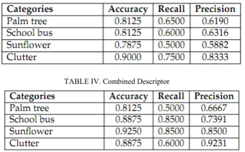
TABLE III. Covariance Descriptor
TABLE IV. Combined Descriptor
IV. CONCLUSION
In this work region covariance descriptor is proposed. But it is not over performing Gray SIFT descriptor on all datasets we worked on. It is over performing on some datasets and underperforming on some other datasets. It still needs further investigations to make use of it in more efficient way. Region Covariance is used as a descriptor with Bag of visual words of model. A 13 dimensional feature vector is taken at each pixel in the region of interest. The features are spatial location, Gaussian kernel with three different
values, first order Gaussian derivatives with two different values, and second order Gaussian derivatives with four different values. Image is represented with a set of bag of visual words. Bag of visual words obtained with Covariance and Gray SIFT descriptors are concatenated.
The performance of different descriptors on different datasets is as follows
• Caltech-3 dataset: It has high inter-class variance and moderate intra-class variance. Combined descriptor is giving better accuracy and recall, whereas Gray SIFT is giving better precision. If we compare on category wise, combined descriptor is better on sunflower, Gray SIFT descriptor is better on Palm-tree and three descriptors are performing equally on school-bus. On the whole, combined descriptor is performing better than remaining two and Gray SIFT descriptor is performing better than covariance descriptor. Here, we can conclude from above observations that combined descriptor still performs better even when intra-class variance is moderate
• Caltech-4 dataset: Combined descriptor performs better than Gray SIFT and Covariance descriptor when the inter-class variance is high and intra-class variance is moderate to low • Animal dataset: All three descriptors are performing poorly when inter-class variance is moderate to low and intra-class variance is high to moderate
REFERENCES
[1] Gabriella Csurka, Christopher R. Dance, Lixin Fan, Jutta Willamowski, Cdric Bray,Visual Categorization with Bags of Key points , InWorkshop on Statistical Learning in Computer Vision, ECCV (2004), 1-22.
[2] Thomas Hofmann, Unsupervised Learning by Probabilistic Latent Semantic Analysis, In Journal of machine Learning (2001), 177-196. [3] Josef Sivic, Bryan C. Russell, Alexei A. Efros, Andrew Zisserman,
William T. Freeman, Discovering objects and their location in images, In IEEE Intl. Conf. on Computer Vision (2005), 370-377.
[4] J.Winn, A. Criminisi and T. Minka, Object Categorization by Learned Universal Visual Dictionary, In ICCV 2005, 1800-1807.
[5] Li Fei-Fei, Pietro Perona, A Bayesian Hierarchical Model for Learning Natural Scene Categories, In CVPR 2005, 524-531.
[6] Yutaka Hirano, Christophe Garcia, Rahul Sukthankar and Anthony Hoogs, Industry and Object Recognition: Applications, Applied Research and Challenges, In Toward Category-Level Object Recognition, Lecture Notes in Computer Science (2006), 49-64. [7] Joseph L. Mundy, Object Recognition in the Geometric Era: A
Retrospective Learning Optimal Compact Codebook for Efficient Object Categorization, In Toward Category-Level Object Recognition, Lecture Notes in Computer Science (2006),
[8] Tinne Tuytelaars and KrystianMikolajczyk, Local Invariant Feature Detectors: A Survey, In Foundations and Trends in Computer Graphics and Vision, NOW Foundation, Vol.3 No. 3 (2007) 177-280.
[9] Ilkay Ulusoy and Christopher M. Bishop, Comparison of Generative and Discriminative Techniques for Object Detection and Classification, In Toward Category-Level Object Recognition, Lecture Notes in Computer Science (2006)
[10] Kristen Grauman (UTA) and Bastian Leibe (ETH Zurich), AAAI 2008 Tutorial on recognition,
[11] Jun Yang, Yu-Gang Jiang, Evaluating Bag-of-Visual-Words Representations in Scene Classification, Proceedings of the international workshop on Workshop on multimedia information retrieval, ACM, 197-206.
[12] Krystian Mikolajczyk, Cordelia Schmid, A performance Evaluation of Local Descriptors, PAMI 2005, 1615-1630.
[13] Marc’ Aurelio Ranzato, Fu-Jie Huang, Y-Lan Bouraeu, Yann LeCun, Unsupervised Learning of Invariant Feature Hierarchies with Applications to Object Recognition, In CVPR 2007, 1-8.
[14] Rob Fergus, New York University, ICML 2008 Tutorial on Recognition, [15] Axel Pinz, Object Categorization, In Foundations and Trends in
Computer Graphics and Vision, NOW Foundation, Vol.1 No.4 (2005) 255-353.
[16] Florent Peronnin, Christpher Dance, Gabrels Csurka, Marco Bressan, Adapted Vocabularies for Generic Visual Categorization, In ECCV, 464-475.
[17] Paul Viola, Michael Jones, Robust Real-time Object Detection, In IJCV 2001
[18] Ivan Laptev, Improving Object Detection with Boosted Histograms, In Image and Vi-sion Computing 2009, 535-544.
[19] David G. Lowe, Distinctive Image Features from Scale-Invariant Key points, In IJCV2004, 91-110.
[20] Jan-Mark Geusebroek, Compact Object Descriptors from Local Color Invariant His-tograms, In British Machine Vision Conference, 2006, 1029-1038.
[21] Oncel Tuzel, Fatih Porikli, and Peter Meer, Region Covariance: A Fast Descriptor forDetection And Classification, In Proc. 9th European Conf. on Computer Vision (2006),589-600.