Influence of module design and membrane compressibility on VMD performance
Jianhua Zhanga*, Jun-De Lib, Mikel Dukea, Manh Hoangc, Zongli Xiec, Andrew Grothd, Chan Tund, Stephen Graya a Institute of Sustainability and Innovation, Victoria University, PO Box 14428, Melbourne, Victoria 8001, Australia b School of Engineering and Science, Victoria University, P.O. Box 14428, Melbourne, Victoria 8001, Australia c CSIRO Materials Science & Engineering, Private bag 33, Clayton South MDC, Victoria 3169, Australia d R&D, Memcor, Siemens, 15 Blackman Crescent, South Windsor, New South Wales, 2756, Australia
* Corresponding author. Tel.: +61 3 9919 7617; fax: +61 3 9919 7696. E-mail address: [email protected]
Abstract
Six modules with different packing densities and lengths were fabricated for conducting vacuum membrane distillation (VMD) experiments. The performances of the modules with different packing densities showed similar results for flux at different temperature and feed velocities. However, shorter modules show both higher flux and global mass transfer coefficient than that of longer modules. It was also found that the increased flux at higher velocity was largely due to the increased average feed temperature rather than reduced temperature polarisation. The flux decay in this study was considered to be caused by gradual compression of the membrane which was confirmed by a compression test. This phenomenon should be noted in the study of VMD, since the pressure difference across the membrane is in general more than 100 kPa and the porosity of the membrane is in general high which results in reduced mechanical strength.
Key words:
Vacuum membrane distillation, module design, membrane compression, heat and mass transfer
1. Introduction
Membrane distillation (MD) is a membrane based thermal process [1, 2], for which the driving force is a vapour pressure difference across the membranes. MD is capable of utilising low grade heat sources to produce (or remove) water at relative low temperature (40 – 80 °C) compared to other thermal processes [3], and is not significantly affected by salt concentration as in Reverse Osmosis. Therefore, MD is a potential alternative for applications such as desalination utilising low grade heat, concentration of thermally sensitive solutions and the treatment of wastewater of high-salt concentration [2].
contact with liquid permeate (Direct Contact Membrane Distillation - DCMD), static air (Air Gap Membrane Distillation - AGMD) or moving gas (Sweep Gas Membrane Distillation - SGMD ) [1, 4, 5].
In DCMD, hollow fibres can provide greater surface area per unit volume than flat sheet configurations, but suffer from poor hydrodynamic conditions on the shell side [6] leading to temperature polarisation and poor performance. Application of hollow fibres in VMD negates these concerns as vacuum may be applied on the shell side minimizing the hydrodynamic issues that may arise in DCMD.
In VMD, the absolute hydrodynamic pressure of the feed stream needs to be controlled so that it is lower than the minimum Liquid Entry Pressure (LEP) to avoid wetting of the membrane and the permeate (vapour) pressure is often maintained below the equilibrium vapour pressure by a vacuum pump. In this configuration the vapour does not condense in the module chamber, instead it is drawn out of the MD module by the vacuum and condenses in an external condenser. The pressure difference between the two sides of the membrane causes convective mass flow through the pores that contributes to the total mass transfer of VMD. Compared with DCMD and AGMD where there is only the diffusive flux of volatile components within the membrane pores, the mass flux of VMD is generally higher than that of other MD configurations when the vapour pressure difference is the same. Heat conduction through the membrane in VMD is in general negligible due to the insulating nature of the vacuum on the permeate side. Thus, the single-pass thermal efficiency of the VMD is higher than that of DCMD and AGMD.
Of the four configurations, VMD has attracted the least attention from researchers [2, 5], and there are little data available on pilot testing. The aims of this work were to understand the effect of membrane compressibility on the performance of VMD, and how the performance of the VMD was affected by hollow fibre packing density, module length, feed velocity, vacuum pressure and feed temperature. The results will serve as a preliminary guide for module design and operational parameter optimisation.
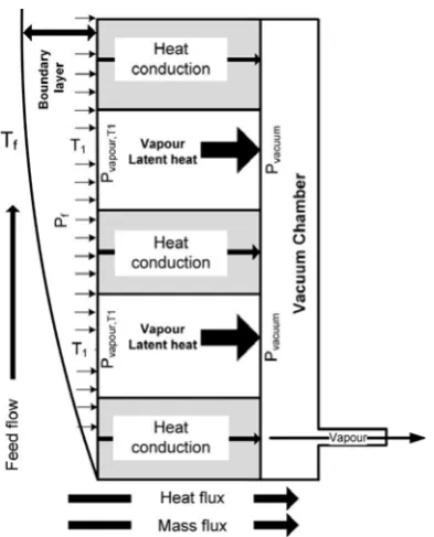
Fig. 1 Schematic diagram of mass and heat transfers in VMD
A schematic diagram of mass and heat transfer across the membrane in VMD is shown in Fig. 1, where Tf and T1 are the bulk and interface temperatures of the feed, Pvapour,T1 and
Pvacuum are the pressures of vapour at feed interface and the vacuum chamber, and Pf is the hydraulic pressure applied on the membrane surface. The mass transfer through a porous MD membrane can be interpreted by three fundamental mechanisms: Knudsen diffusion, molecular diffusion and Poiseuille flow [7, 8]. The Knudsen number (Kn) defined as:
d l
Kn / (1)
and is used to judge the dominating mechanism of the mass transfer in the pores. Here, l is the mean free path of the transferred gas molecules and d is the mean pore diameter of the membrane.
In membrane distillation, the pores size of hydrophobic membranes used are generally in the range of 0.1 to 1.0 µm [9] and the mean free path of the water is 0.11 µm at 60 °C under atmospheric pressure [10]. Thus, the Knudsen number is in the range of 0.11 - 0.55.
within the pores is Poiseuille flow - Knudsen diffusion transition mechanism [2, 10] and can be simplified as:
P C
Flux (2)
where C is the global mass transfer coefficient, PPvapour,Tf.mean Pvacuum is the vapour pressure difference between that in the vacuum chamber and that vapour pressure calculated at temperature Tf,mean (mean temperature of the feed flow).
The heat transfer from the bulk feed stream to the vacuum chamber across a hollow fibre wall can be expressed as:
A T T b A PH C A T T T T FC
Qf,transfer p( f,i f,o)f,mean( f,mean 1,mean) latent ( 1,mean shell) (3)
where Qf,transfer is the absolute overall heat transfer, F is the mass flowrate of the feed, Cp is the specific heat of the feed, A is the membrane area, briln(ro /ri) is nominal wall thickness, Hlatent is the latent heat of the permeate, αf is the convective heat transfer coefficient, Tshell is the temperature in the vacuum chamber, ri and ro are the inner and outer radii of the hollow fibre, and λ is the thermal conductivity of the hollow fibre.
The convective heat transfer coefficient can be defined as:
i w
f d
Nu
(4)
Here, where Nu is Nusselt number, di is the inner diameter of the hollow fibre and λw is the thermal conductivity of the water.
The global heat transfer coefficient αglobal across the membrane can be calculated based on overall heat balance:
A T T AH Flux T T
FCp( f,i f,o) latent global( f,mean shell) (5)
The ratio of the thermal energy used for evaporation to the total thermal energy lost from the feed stream can be calculated by:
% 100 ) ( , , o f i f p latent P K T T FC AH N
E (6)
The temperature polarisation coefficient (TPC) in VDM can be defined as:
shell mean f shell mean T T T T TPC , ,
1 (7)
3. Experimental
3.1 Experimental conditions
with the gas permeability method described by [2] for membrane A and B were 8.95×10⁻⁴ and 1.75×10⁻³. Since the thickness, pore size and porosity of the membranes A and B were similar, it indicates that the tortuosity of membrane A was about twice that of membrane B.
Table 1
Specification of the fabricated modules
membrane Module length
(mm)
Packing density
(%) Fibre pieces
A
ID
(mm) (mm) OD
250 32 63
250 40 80
0.8 1.5 250 48 97
B
ID (mm)
OD (mm)
150 40 80
250 40 80
0.7 1.4 350 40 80
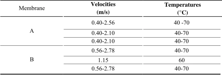
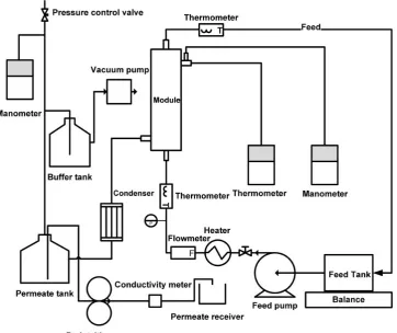
The VMD experimental setup is shown in Fig. 2. Five or six different velocities and four different temperatures were tested for each module as listed in Table 2. Each experiment was stabilised for 1 hour before the experimental results were recorded and lasted no less than 3 h. The membrane was relaxed overnight (at least eight hours) between tests using the same module. The feed reservoir weight was recorded every 15 to 30 min. The relationship between the flux and the vacuum pressure was also studied using a module length of 25 cm with membrane B. The vapour permeate was condensed by chilled water at 3.6 ºC in a heat exchange. The flux was calculated based on the weight reduction of the feed reservoir. Tap water with conductivity of 120 μS was used as feed, and salt rejection in all results reported here was greater than 99%.
Table 2
Experimental conditions for different membrane packing densities and module lengths
Membrane Velocities
(m/s)
Temperatures (°C)
A
0.40-2.56 40 -70
0.40-2.10 40-70
0.40-2.10 40-70
B
0.56-2.78 40-70
1.15 60
Fig. 2 Schematic diagram of the experimeatal setup for VMD
3.2 Liquid Entry pressure (LEP) and membrane compressibility tests
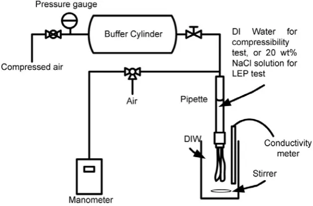
The apparatus as outlined in Fig. 3 was used to test the LEP and compressibility of the hollow fibre membranes. In the test, compressed air was injected into a buffer cylinder. A pressure gauge was used to monitor the pressure of the injected air. An increment of 10 kPa was used to increase the pressure between readings. After the pressure reached the required value, the upstream valve was closed and the downstream valve was opened. Then, the air pressure was applied to the deionised water in a pipette (accuracy 0.005 mL) connected to a hollow fibre module.
In the LEP test, 20 wt% NaCl solution was filled in the pipette. Conductivity changes of 200 mL deionised water (DIW) at 20 ºC in the stirred beaker surrounding the hollow fibre module was monitored by a conductivity meter (HANNA HI 9032), and the approximate constant pressure (±0.1 Pa) was maintained for 1 min at each test pressure to allow detection of any transport of NaCl through the membrane. This technique was based on the technique described in [13]. The calculated LEP of both membranes was 185 ± 10 kPa based on the method presented [13].
pipette with silicon tubing, a blank test was performed to account for the volume change associated with the compressibility of the silicon tube. The hollow fibre was also soaked in deionised water at 20 ºC to avoid any volume change caused by evaporation, which occurred if the module was placed in air. The volume was recorded when there was no obvious volume change for a 30 second period, and the pressure was increased in 10 kPa increments from 10 to 100 kPa. The test was conducted for two different membranes due to availability (Fibre 1 and Fibre 2 had similar characteristics to membrane A and B, but was from a different fabrication batch from the same laboratory scale machine) and repeated three times for each membrane sample.
Fig. 3 Schematic diagram of the LEP and compressibility test apparatus
4. Results and discussion
4.1 Influence of module design on VMD performance
The experiments were conducted by comparing the performance of assembled membrane modules with different membrane packing densities (membrane A) and different membrane lengths (membrane B) at various velocities and temperatures. Based on the experimental variability and the deviation around the calculated mean value, the error bars were ±10% for the flux and mass transfer coefficients, ±5% for vacuum pressure, ±3% for thermal efficiency, ±2% for velocities, and ±1% for temperatures, respectively.
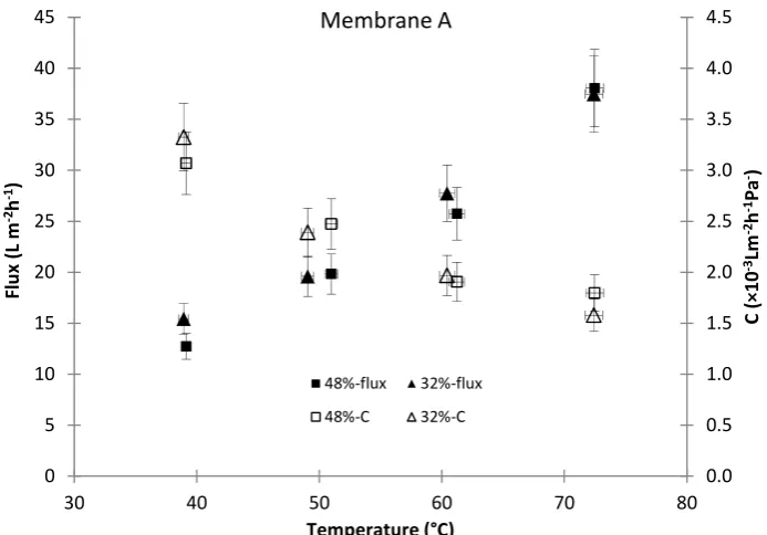
Figs. 4 and 5 show the flux and thermal efficiency of the modules (membrane A) with different packing densities at different velocities and temperatures. It was found from these results that the packing densities of the hollow fibre membranes did not show any obvious influence on the flux of the modules.
coefficient and vapour pressure difference. As the global mass transfer coefficient (C) only varied slightly at different stream velocities, the flux variation at different velocities was largely due to changes of the vapour pressure difference as the average bulk feed temperature increased at higher velocity due to changes in the temperature profile. In calculating the global mass transfer coefficient, these changes in temperature profile and resultant vapour pressure differences are accounted for, so the global mass transfer coefficient (C) was mainly determined by the membrane properties and the mass transfer resistance in the boundary layer (theoretically thinned at higher velocity) [8, 13]. The global mass transfer coefficient rose by only 20% and the flux by 50% (packing density of 48%) in the tested velocity range. However, a 53% increase of the global mass transfer coefficient and 73% of flux were reported in paper [13] where hollow fibre DCMD was studied. Therefore, it can be concluded that the boundary layer thickness had a relatively small influence on flux in hollow fibre VMD, particularly compared with DCMD results from our previous study.
0.0 0.5 1.0 1.5 2.0 2.5 3.0 3.5 4.0 4.5
0 5 10 15 20 25 30 35 40 45
0.0 0.5 1.0 1.5 2.0 2.5 3.0
C
(×
1
0
‐
3Lm
‐
2h
‐
1Pa
‐
1)
Fl
ux
(L
m
‐
2h
‐
1)
Velocity (m/s)
Membrane A
48%‐flux 32%‐flux
48%‐C 32%‐C
0.0 0.5 1.0 1.5 2.0 2.5 3.0 3.5 4.0 4.5 0 5 10 15 20 25 30 35 40 45
30 40 50 60 70 80
C (×10 ‐ 3Lm ‐ 2h ‐ 1Pa ‐) Fl u x (L m ‐ 2h ‐ 1) Temperature (°C)
Membrane A
48%‐flux 32%‐flux
48%‐C 32%‐C
b. Flux at different temperatures (Feed velocity = 0.81 ± 0.05 m/s)
Fig. 4 Flux and mass transfer coefficients of modules with different packing densities (membrane A: vacuum pressure = 3 ± 1 kPa absolute)
Figs. 4a with 4b show the global mass transfer coefficients were affected more by the feed temperature than that of the feed velocity, which is opposite to the findings for DCMD [8]. At different feed temperatures as shown in Fig. 4b, the flux for VMD increased exponentially, which is similar to the findings in DCMD [5, 14]. The global mass transfer coefficient declined with temperature due to increased temperature polarisation on the feed side [14]. As a rough estimation, based on Leveque’s equation (Nu 1.615(RePrd /L)1/3
i
for Reynolds
number <2100, laminar flow) [15] the calculated Nusselt numbers at different temperatures were about the same under the experimental conditions (the ratio is between 0.99 to 1.02). Therefore, based on Eq. (4), it can be found that the convective heat transfer coefficient (αf) is only affected by the water thermal conductivity and increases roughly by 7% as the temperature rises from 40 to 70 ºC [16]. However, the flux at 70 ºC was 2.8 times of the flux at 40 ºC. Therefore, based on Eq. (5), the calculated temperature difference between that of the bulk feed flow (Tf,mean) and that of the membrane interface (T1,mean) was increased 2.8 times when temperature increase from 40 to 70 ºC (the sensible heat loss only account for 1 - 5% of the total heat loss from the feed). Eq. (7) can be converted to:
shell mean f mean f mean shell mean f mean f mean f shell mean shell mean f shell mean T T T T T T T T T T T T T T TPC , , , 1 , , , , 1 , ,
1 1 (8)
As the mean shell temperatures measured experimentally at feed temperatures of 40 ºC (Tf,mean = 37 ºC) and 70 ºC (Tf,mean = 65 ºC) were respectively 25 ºC and 42 ºC and assuming a = T1,mean – Tf,mean at 40 ºC, then
12 1 25 37
1 a a
TPC
(9)
at 70 ºC:
1 . 6 1 42 65
8 . 2
1 a a
TPC
(10)
Since a is greater than 0, it can be found the calculated TPC at 70 ºC should be smaller than that of at 40 ºC, which means the temperature polarisation was worse at 70 ºC. The Reynolds number of 1600 at 70 ºC feed temperature was higher than the Reynolds number of 950 at 40 ºC feed temperature, so there was greater turbulence at 70 ˚C feed temperature. Therefore, the raised temperature polarisation with the increasing temperature was largely caused by increased heat transfer across the boundary layer due to the higher flux, as the hydrodynamic boundary layer effects improved at higher temperature.
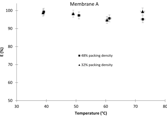
As shown in Figs. 5a and 5b, the thermal efficiency of the VMD was almost independent of the velocities and temperatures, in which the average values were all greater than 90% and the maximum values were almost 98% under all tested conditions. The nearly constant thermal efficiency under the varied conditions is due to the negligible sensible heat loss in VMD [2, 17-19], which is different from that in DCMD [8, 13] where increases in thermal efficiency occurred with increasing feed temperature and velocity.
50 60 70 80 90 100
0.0 0.5 1.0 1.5 2.0 2.5 3.0
E
(%)
Velocity (m/s)
Membrane A
48% packing density
32% packing density
50 60 70 80 90 100
30 40 50 60 70 80
E
(%
)
Temperature (°C)
Membrane A
48% packing density
32% packing density
b. Thermal efficiency at different temperatures (velocity = 0.81 ± 0.05 m/s)
Fig. 5 Thermal efficiency of modules with different packing densities (membrane A: vacuum pressure = 3 ± 1 kPa absolute)
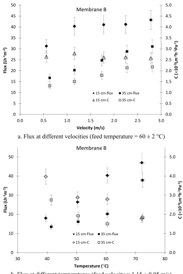
The flux and global mass transfer coefficients of the modules with different lengths (membrane B) at different velocities and temperatures are shown in Figs. 6a and 6b, which shows similar trends to Fig. 4a and 4b.
The global mass transfer coefficients declined with increasing temperature (Fig 6b), similar to the trends shown in Fig 4b. Increased temperature polarisation was considered to occur with increased feed temperature because of the greater rate of evaporation occurring at the membrane surface due to the higher temperature and resultant vapour pressure.
0.0 0.5 1.0 1.5 2.0 2.5 3.0 3.5 4.0 4.5 5.0 0 5 10 15 20 25 30 35 40 45 50
0.0 0.5 1.0 1.5 2.0 2.5 3.0
C ( × 10 ‐ 3Lm ‐ 2h ‐ 1Pa ‐ 1) Flu x (L h ‐ 1m ‐ 2) Velocity (m/s)
Membrane B
15 cm‐flux 35 cm‐flux 15 cm‐C 35 cm‐C
a. Flux at different velocities (feed temperature = 60 ± 2 °C)
0.0 1.0 2.0 3.0 4.0 5.0 0 10 20 30 40 50
30 40 50 60 70 80
C ( × 10 ‐ 3Lm ‐ 2h ‐ 1Pa ‐ 1) Fl u x (Lh ‐ 1m ‐ 2)
Temperature (°C)
Membrane B
15 cm‐Flux 35 cm‐flux
15 cm‐C 35 cm‐C
b. Flux at different temperatures (feed velocity = 1.15 ± 0.05 m/s)
Fig. 6 Flux of modules with different lengths (membrane B: vacuum pressure = 3 ± 1 kPa absolute)
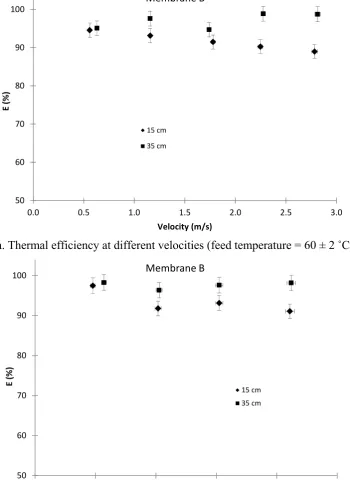
slightly affected by the experimental temperatures and velocities, with all results being within the range of experimental error.
50 60 70 80 90 100
0.0 0.5 1.0 1.5 2.0 2.5 3.0
E
(%)
Velocity (m/s)
Membrane B
15 cm
35 cm
a. Thermal efficiency at different velocities (feed temperature = 60 ± 2 ˚C)
50 60 70 80 90 100
30 40 50 60 70 80
E
(%
)
Temperature (°C)
Membrane B
15 cm 35 cm
b. Thermal efficiency at different temperatures (1.15 ± 0.05 m/s) Fig. 7 Thermal efficiency of modules with different membrane lengths
(membrane B: vacuum pressure = 3 ± 1 kPa absolute)
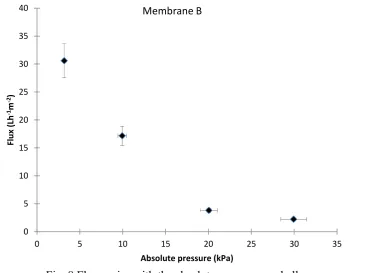
the pressure at pore interface on the permeate side, and a dramatic increase in vapour flow occurs as the water boils. As the air in the pore will be completely replaced by the water vapour, the dominant transfer mechanism changes from molecular - Knudsen diffusion to Poiseuille flow - Knudsen diffusion transition mechanism [2].
0 5 10 15 20 25 30 35 40
0 5 10 15 20 25 30 35
Flu
x
(Lh
‐
1m
‐
2)
Absolute pressure (kPa)
Membrane B
Fig. 8 Flux varies with the absolute pressure on shell
(membrane B: feed temperature = 60 ± 2 ºC, feed velocity = 1.15 ± 0.05 m/s, membrane length = 25 cm)
4.2 Influence of membrane compressibility on VMD performance
0 5 10 15 20 25 30 35 40
0 50 100 150 200 250 300 350
Flu
x
(Lm
‐
2h
‐
1)
t (min)
Membrane A
v=2.6 m/s
v=2.1 m/s
v=1.7 m/s
v=0.8 m/s
v=0.4 m/s
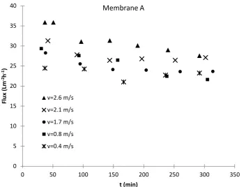
a. Flux decline with time at different velocities (feed temperature = 60 ± 2 ºC)
0 5 10 15 20 25 30 35 40
0 50 100 150 200 250 300 350
Flux
(Lm
‐
2h
‐
1)
t (min)
Membrane A
T=70°C
T=50°C
T=40°C
b. Flux decline with time at different temperatures (feed velocity = 1.15 ± 0.05 m/s)
Fig. 9 Flux decline with time
(membrane A: packing density = 40%, vacuum pressure = 3 ± 1 kPa absolute)
was found that the flux also declined when deionised water was used as feed, and there was no observed flux difference between the deionised water and tap water (TW) feeds.
0 5 10 15 20 25 30 35 40
0 50 100 150 200 250 300
Fl
u
x
(L
m
‐
2h
‐
1)
Time (min)
Membrane A
DIW TW
Fig. 10 Comparison of flux decline of DIW to TW
(Hollow fibre A: packing density = 40%, inlet temperature = 60 ± 2 °C, stream velocity = 1.7 ± 0.05 m/s, vacuum pressure = 3 ± 1 kPa absolute)
y = ‐3.9E‐04x + 3.3E‐03 R² = 9.8E‐01
y = ‐1.9E‐04x ‐5.4E‐04 R² = 9.5E‐01
y = ‐1.6E‐04x ‐2.6E‐04 R² = 9.2E‐01
‐8.0
‐7.0
‐6.0
‐5.0
‐4.0
‐3.0
‐2.0
‐1.0
0.0 ‐0.040
‐0.035
‐0.030
‐0.025
‐0.020
‐0.015
‐0.010
‐0.005
0.000
0 20 40 60 80 100 120
Calc
u
lated
memb
rane
thickness
chang
e
(%)
Volu
me
cha
n
ge
(m
L)
Pressure difference across the membrane (kPa) Total valume change (Fibre 1)
Total volume change (Fibre 2) Blank test
Fibre 1: Calculated membrane thickness change with pressure Fibre 2: Calculated membrane thickness change with pressure
Fig. 11 Membrane volume change during compression in water at 20 ˚C
0.0 0.5 1.0 1.5 2.0 2.5 3.0 3.5 4.0
0 1 2 3 4 5 6 7
100 120 140 160 180 200
Ve
lo
ci
ty
(m/s
)
Gl
ob
al
hea
t
tra
n
sf
er
coeff
ici
ent
(kW
m
‐
2K
‐
1)
Pressure (kPa)
Membrane A
Global heat transfer coefficient
Velocity
Fig. 12 Relationship between global heat transfer coefficient and pressure difference across membrane
(membrane A: packing density = 48%)
The compressed membrane will also show increased thermal conductivity as found in [20, 21]. The global heat transfer coefficients for the hollow fibre membranes in this study were calculated by Eq. (5), and its relationship against velocity and feed pressure is shown in Fig. 12. Based on Leveque equation and Eq. (4), the Nusselt number at feed velocity of 1.68 m/s was about 1.54 times of that of 0.42 m/s under the same conditions as data shown in Fig. 12. However, the global thermal conductivity at 1.68 m/s was about 3.43 times that at 0.42 m/s. Therefore, the variation of the global heat transfer coefficient was caused by the change of thermal conductivity of the hollow fibre. The global heat transfer coefficient (thermal conductivity) increased fast initially with escalating pressure, and plateaued when the pressure difference increased above 150 kPa. The plateau maybe represent that the membrane was approaching complete deformation.
Based on this finding, it was speculated that the smaller global mass transfer coefficients of the long module in Fig. 6 may also be due to the higher pressure drop along the module (causing greater membrane compression) than that of the short module.
kPa respectively at 70, 50 and 40 ºC). Therefore, the results are consistent with the extent of membrane compression being largely affected by the hydraulic pressure in the tested temperature range.
In Fig. 10 (membrane A), the flux did not change greatly between the two tests (there were 4 experiments: 2 repeats of each experiment), although there was the flux decline during the experiment. However, as shown in Fig. 13 for membrane B, permanent flux loss of more than 25% was observed. These results suggest membrane A was able to recover to its initial flux performance upon rest, while for membrane B there was irreversible flux loss. The recoverability of membrane flux may be related to the membrane structure, with the lower permeability and higher tortuosity membrane showing better recoverability. However, further research is required to understand this phenomenon.
0 5 10 15 20 25
0.0 0.5 1.0 1.5 2.0 2.5 3.0
Flux
(L
m
‐
2h
‐
1)
Velocity (m/s)
Membrane B
First experimental series Second experimental series
Fig.13 Experiments repeated at different velocities
(membrane B: feed temperature = 60 ± 2 ºC, membrane length = 25 cm, vacuum pressure = 3 ± 1 kPa absolute)
5. Conclusion
Six different modules were fabricated for the VMD experiments. The performances of the modules with different packing densities showed similar results in flux at different temperature and feed velocities. However, the shorter module showed higher flux and global mass transfer coefficient than that of the longer module.
greater than 100 kPa and the porosity of the membranes is high resulting in reduced mechanical strength.
The recoverability of membranes A and B after compression varied, possibly due to differences in the pore structure. Membrane A that had the lower gas permeability and higher tortuosity appeared to fully recover after relaxation overnight, while membrane B suffered some permanent flux loss. This should also be noted, since it may be confused with permanent flux loss due to the fouling.
It was found that increased flux at higher velocity was largely due to the increased average feed temperature rather than reduced temperature polarisation.
A shorter module with high packing density is suggested to obtain a high yield per unit volume based on this study of hollow fibre VMD.
If the single pass recovery is important, using a slow velocity rather than a very long membrane to get a longer residency time may be a better choice, based on the influence of stream velocity and membrane length on the thermal efficiency.
Acknowledgements
The authors acknowledge the financial support of the National Centre of Excellence for Desalination Australia which is funded by the Australian Government through the Water for the Future initiative.
Nomenclature
A Membrane area (m2)
Cp Heat capacity (J/mol.K) F Volumetric flow rate (m3/s)
Kn Knudsen number
l Molecular path (µm)
λ Thermal conductivity (W/m)
M Molecular weight (g/mol)
P Pressure (Pa)
R Gas constant (J/mol.K)
Re Reynolds number
T Temperature (K)
v Linear velocity (m/s)
Qf,transfer absolute overall heat transfer (W)
ri, ro Inner and outer radius of the hollow fibre membrane (m) Subscript
1 Feed interface
f Feed
h Hot side
f,i Feed inlet
f,o Feed outlet
mean Average from the fibre inlet to outlet
[1] K. W. Lawson, D. R. Lloyd, Membrane distillation, Journal of Membrane Science. 124 (1997) 1‐25. [2] Z. Lei, B. Chen, Z. Ding, Membrane distillation, in: Z. Lei, B. Chen, Z. Ding (Eds.), Special Distillation Processes, Elsevier Science, Amsterdam, 2005, pp. 241‐319.
[3] N. Dow, S. Gray, J.‐d. Li, J. Zhang, E. Ostarcevic, A. Liubinas, P. Atherton, D. Halliwell, M. Duke. Power station water recycling using membrane distillation ‐ A plant trial. in Ozwater. 2012. Sydney. [4] W. T. Hanbury, T. Hodgkiess, Membrane distillation ‐ an assessment, Desalination. 56 (1985) 287‐ 297.
[5] E. Curcio, E. Drioli, Membrane Distillation and Related Operations: A Review, Separation and Purification Reviews. 34 (2005) 35 ‐ 86.
[6] X. Yang, R. Wang, L. Shi, A. G. Fane, M. Debowski, Performance improvement of PVDF hollow fiber‐based membrane distillation process, Journal of Membrane Science. 369 (2011) 437‐447. [7] A. O. Imdakm, T. Matsuura, A Monte Carlo simulation model for membrane distillation processes: direct contact (MD), Journal of Membrane Science. 237 (2004) 51‐59.
[8] J. Zhang, J.‐D. Li, M. Duke, Z. Xie, S. Gray, Performance of asymmetric hollow fibre membranes in membrane distillation under various configurations and vacuum enhancement, Journal of
Membrane Science. 362 (2010) 517‐528.
[9] A. M. Alklaibi, N. Lior, Membrane‐distillation desalination: Status and potential, Desalination. 171 (2005) 111‐131.
[10] J. Phattaranawik, R. Jiraratananon, A. G. Fane, Effect of pore size distribution and air flux on mass transport in direct contact membrane distillation, Journal of Membrane Science. 215 (2003) 75‐85.
[11] M. A. Izquierdo‐Gil, G. Jonsson, Factors affecting flux and ethanol separation performance in vacuum membrane distillation (VMD), Journal of Membrane Science. 214 (2003) 113‐130. [12] R. W. Schofield, A. G. Fane, C. J. D. Fell, Gas and vapour transport through microporous membranes. II. Membrane distillation, Journal of Membrane Science. 53 (1990) 173‐185.
[13] J. Zhang, N. Dow, M. Duke, E. Ostarcevic, J.‐D. Li, S. Gray, Identification of material and physical features of membrane distillation membranes for high performance desalination, Journal of Membrane Science. 349 (2010) 295‐303.
[14] J. Phattaranawik, R. Jiraratananon, Direct contact membrane distillation: effect of mass transfer on heat transfer, Journal of Membrane Science. 188 (2001) 137‐143.
[15] H. Martin, The generalized Lévêque equation and its practical use for the prediction of heat and mass transfer rates from pressure drop, Chemical Engineering Science. 57 (2002) 3217‐3223. [16] M. L. V. Ramires, C. Nieto de Castro, Y. Nagasaka, A. Nagashima, M. J. Assael, W. A. Wakeham, Standard reference data for the thermal conductivity of water, Journal of Physical and Chemical Reference Data. 24 (1995) 1377‐1382.
[17] B. Li, K. K. Sirkar, Novel membrane and device for vacuum membrane distillation‐based desalination process, Journal of Membrane Science. 257 (2005) 60‐75.
[18] S. Bandini, C. Gostoli, G. C. Sarti, Separation efficiency in vacuum membrane distillation, Journal of Membrane Science. 73 (1992) 217‐229.
[19] T. Mohammadi, M. Akbarabadi, Separation of ethylene glycol solution by vacuum membrane distillation (VMD), Desalination. 181 (2005) 35‐41.
[20] J. Zhang, S. Gray, J.‐D. Li, Modelling heat and mass transfers in DCMD using compressible membranes, Journal of Membrane Science. 387–388 (2012) 7‐16.
[21] J. Zhang, J.‐D. Li, S. Gray, Effect of applied pressure on performance of PTFE membrane in DCMD, Journal of Membrane Science. 369 (2011) 514‐525.