Page 1 of 20 Cite this article as:
Debnath, A.K., Blackman, R., and Haworth, N. (2014) A Tobit model for analyzing speed limit compliance in work zones. Safety Science, Vol. 70, pp. 367-377.
A TOBIT MODEL FOR ANALYZING SPEED LIMIT COMPLIANCE IN
WORK ZONES
Ashim Kumar Debnath1*, Ross Blackman2, Narelle Haworth3
1
Centre for Accident Research and Road Safety – Queensland K Block, Queensland University of Technology
130 Victoria Park Rd, Kelvin Grove, QLD 4059, Australia Tel: +61731388423, Fax: +61731380111
Email: ashim.debnath@qut.edu.au
2
Centre for Accident Research and Road Safety – Queensland K Block, Queensland University of Technology
130 Victoria Park Rd, Kelvin Grove, QLD 4059, Australia Tel: +61731384638, Fax: +61731380111
Email: ross.blackman@qut.edu.au
3
Centre for Accident Research and Road Safety – Queensland K Block, Queensland University of Technology
130 Victoria Park Rd, Kelvin Grove, QLD 4059, Australia Tel: +61731388417, Fax: +61731380111
Email: n.haworth@qut.edu.au
*
Corresponding author
ABSTRACT
Poor compliance with speed limits is a serious safety concern in work zones. Most studies of work zone speeds have focused on descriptive analyses and statistical testing without
Page 2 of 20 of surrounding vehicles were non-compliant. Light vehicles and their followers were also more likely to speed than others. Speeding was more common and greater in magnitude upstream than in the activity area, with higher compliance rates close to the end of the activity area and close to stop/slow traffic controllers. The modeling technique and results have great potential to assist in deployment of appropriate countermeasures by better identifying the traffic characteristics associated with speeding and the locations of lower compliance.
Keywords: work zone safety, Tobit regression, roadworks, speeding, speed limit.
1. INTRODUCTION
Excessive and differential speeds are major contributing factors in work zone crashes and driver compliance with work zone speed limits is generally poor (Allpress and Leland Jr, 2010; Garber and Zhao, 2002). Speeding was cited as a contributing factor in 42% of work zone crashes in Texas (Brewer et al., 2006), 7% of fatal crashes in Georgia (Daniel et al., 2000), and 25% and 16% of fatal and injury crashes respectively in Kansas (Bai and Li, 2011). As well as increasing crash risk, exceeding work zone speed limits also increases the severity of crashes when they occur. These points apply almost universally to highway work zones regardless of their location and characteristics, as demonstrated in a large number of studies worldwide (Allpress and Leland Jr, 2010; Brewer et al., 2006; Hajbabaie et al., 2011a; Haworth et al., 2002; Li and Bai, 2008; Meng et al., 2010).
Despite the numerous studies of work zone speed characteristics and evaluations of safety treatments, two key gaps remain in current knowledge about work zone speed limit
compliance. First, there is no comprehensive technique for modeling both the probability and magnitude of speed limit compliance in work zones. Most studies have analyzed magnitude of compliance using basic inferential statistics of speed and speed limit compliance.
However, to better identify the speeders, speeding prone locations, and traffic characteristics related to speeding, it is necessary to develop an appropriate regression modeling technique which is able to model both the probability and the magnitude of non-compliance. Second, most analyses of work zone speeds have not accounted for the effects of vehicle and traffic characteristics on compliance levels, arguably because of not using regression techniques in their analyses. As a result, little is known about how the characteristics of surrounding traffic and the presence of platoons influence speeds in work zones.
This paper aims to address the two key gaps in literature by developing an innovative
technique for modeling both the probability and magnitude of speed limit compliance in work zones while controlling for the effects of different vehicle and traffic related factors. The resulting Tobit regression model is illustrated using speed data collected from multiple points in three long-term work zones in Queensland, Australia. The robustness of the technique is demonstrated by calibrating the model with data from different traffic conditions of the three work zones. The modeling technique is the key contribution of this paper, while the findings have great potential to assist in development and evaluation of appropriate speed reduction measures by better identifying high-risk speeders, locations of speeding, and traffic
Page 3 of 20 2. LITERATURE REVIEW OF WORK ZONE SPEED MODELING TECHNIQUES
Many studies have analyzed travel speeds in work zones to both understand the baseline speed characteristics and to evaluate the speed reduction potential of countermeasures. For example, Bham and Mohammadi (2011) examined baseline free-flow speeds and compliance levels of car and trucks in four Missouri work zones using descriptive statistics and t-tests. In an older Illinois study, Benekohal et al. (1992) used descriptive statistics of speeds and speed limit compliance to group the behavior of drivers into four distinct categories: (1)
considerable speed reductions after passing the first speed reduction sign (63% of drivers), (2) reduced speeds close to the actual work location (11% of drivers), (3) unchanged travel speeds (11% of drivers), and (4) no significant pattern (15% of drivers).
A range of analysis techniques have been used to evaluate the effectiveness of speed control measures in work zones (see Debnath et al., 2012 for a review of related literature). In an evaluation study of perceptual countermeasures using traffic cones, Allpress and Leland Jr (2010) analyzed before and after free flow speeds at three points in a New Zealand highway work zone using one-way ANOVA and Tukey’s Honestly Significant Difference post hoc tests (HSD) without distinguishing between vehicle types. Bai and Li (2011) analyzed the speeds of the first two vehicles in a traffic queue using ANOVA and two-sample t-tests to measure the speed reductions associated with using an Emergency Flasher Traffic Control Device. The effects of police and photo-radar enforcement in two Illinois work zones were examined using t-tests, Chi Square, Kolmogorov-Smirnov tests, and Least Significant Difference tests (Benekohal et al., 2010). Temporal and spatial effects of the measures were evaluated using two indicators: mean speed and degree of speeding (at four levels: percentage of vehicles exceeding speed limits, exceeding up to 5 mph, exceeding by 5-10 mph, and exceeding by more than 10 mph) for each vehicle type. Bai et al. (2010) analyzed speed reductions in response to temporary signage in two Kansas highway work zones using descriptive statistics of speed change and ANOVA tests. Brewer et al. (2006) analyzed speed data collected from six points in two Texas highway work zones using mean, 85th percentile, and standard deviation of speed, and percentage of compliant vehicles. Wang et al. (2003) also analyzed speed data from three Georgia work zones using t-test, Bartlett’s test, ANOVA, and Tukey’s HSD test.
The foregoing review shows that most studies of work zone speeds have presented statistical summaries and basic inferential statistics of speed and speed limit compliance data without examining the effects of many potential influencing factors. Travel speeds do not necessarily depend only on a single factor (e.g., day/night, type of vehicle), but are likely to be
influenced by characteristics of vehicles and their surrounding traffic as well. Several studies (e.g., Bai et al., 2010; Benekohal et al., 1992; Benekohal et al., 2010; Debnath et al., 2014) have demonstrated that travel speeds of cars differ from those of trucks. In addition, Morgan et al. (2010) found that the presence of a lead vehicle has significant effects on follower vehicles’ speeds. An evaluation of pilot car operation (Debnath et al., 2014) reported that travel speeds vary according to traffic volumes, gaps from lead vehicles, time of day, and proportions of medium and heavy vehicles. Findings from these studies indicate that the effects of vehicular and traffic characteristics need to be accounted for in order to comprehensively model travel speeds and speed limit compliance in work zones.
Page 4 of 20 While this modeling approach can account for the effects of vehicular and traffic
characteristics on speed limit non-compliance, the magnitude of non-compliance is not captured in the model. Specifically, the model does not differentiate between the non-compliant drivers exceeding speed limits by a large amount and those exceeding by a small amount. Since an increase in speed increases the likelihood of a crash and the severity of a crash when it occurs (Aarts and van Schagen, 2006; Meng et al., 2010), it is important to account for both the probability and magnitude of non-compliance with speed limits in safety analyses.
3. STATISTICAL MODELING METHOD
To examine how different characteristics of vehicles and their surrounding traffic affect driver speeds, it is necessary to use appropriate regression models. In addition, as discussed earlier, from a safety perspective it is important to account for both the probability and the magnitude of non-compliance with speed limits in speed data modeling. A possible way of modeling this problem is transforming the speed values to ‘excess speed’ (i.e., measured speed – speed limit) which would give positive values for the non-compliant drivers and negative or zero values for the compliant drivers. The non-compliant drivers are of key concern in terms of safety improvement in work zones. However, to understand the degree of non-compliance, it is necessary to analyze the speed profiles of the compliant drivers as well.
A Tobit regression model (Tobin, 1958) which models dependent variables with censored data is an appropriate technique for modeling the excess speed data. In the Tobit model framework, the observations of compliant drivers can be clustered at a threshold value of zero (which is termed as left censored in standard Tobit model literature) and those of
compliant drivers can be kept as continuous data to represent the magnitude of non-compliance.
The Tobit model can be expressed as (for speed observation i)
𝑌𝑖∗ = 𝜷𝑿𝑖+ 𝜀𝑖, 𝑖 = 1,2, … , 𝑁 (1)
𝑌𝑖 = 𝑌𝑖∗ 𝑖𝑓 𝑌𝑖∗ > 0 (2)
𝑌𝑖 = 0 𝑖𝑓 𝑌𝑖∗ ≤ 0 (3)
Where 𝑌𝑖 is the dependent variable (speed above the posted limit) which is measured using a latent variable 𝑌𝑖∗ for positive values and censored otherwise, 𝜷 is a vector of estimable parameters, 𝑿𝑖 is a vector of explanatory variables, 𝜀𝑖 is a normally and independently distributed error term with zero mean and constant variance 𝜎2, and N is the number of observations. A detailed description of the Tobit model can be found in Washington et al. (2011).
To estimate the marginal effects of the independent variables, the change in the expected value for cases above zero (𝜕𝐸[𝑌′] 𝜕𝑋⁄ 𝑘) and the change in the cumulative probability of being above zero (𝜕𝐹(𝑧) 𝜕𝑋⁄ 𝑘) for a specific independent variable 𝑋𝑘 are calculated using the following expressions (removing the subscript i for simplification):
𝜕𝐸�𝑌′�
𝜕𝑋𝑘 = 𝛽𝑘�1 − 𝑧
𝑓(𝑧) 𝐹(𝑧)−
𝑓(𝑧)2
Page 5 of 20 𝜕𝐹(𝑧)
𝜕𝑋𝑘 = 𝛽𝑘 𝑓(𝑧)
𝜎 (5)
where 𝐸[𝑌′] = 𝐸[𝑌|𝑌 > 0], 𝑌′ denotes the non-censored observations (i.e., positive values of excess speed), 𝑧 is the 𝑧-score associated with the area under the normal curve, 𝐹(𝑧) is the cumulative normal distribution function, and 𝑓(𝑧)is the unit normal density. The changes were obtained by computing the effect of a unit change in a continuous explanatory variable from its mean value or a change from 0 to 1 for a binary variable while keeping all other variables at their means. In case of variables with more than two categories, the changes were computed on the basis of category change from 0 to 1, whereas the other categories of the variable were kept at 0 and all other variables at their means.
Overall goodness of fit of the model is assessed using Maddala Pseudo R2 (Maddala, 1983) which is expressed as 1 − 𝐸𝑋𝑃[2(𝐿𝐿(0) − 𝐿𝐿(𝛽))/𝑁], where 𝐿𝐿(0) and 𝐿𝐿(𝛽) are the log-likelihood at zero and at convergence respectively.
It should be noted that the standard assumptions of a linear regression model apply to a Tobit model. The assumptions include dependent variable to be continuous, linear relationship between dependent variable and independent variables, independently and randomly sampled observations, non-autocorrelated disturbance terms, uncorrelated disturbances and
independent variables, approximately normally distributed disturbance terms with zero mean and constant variance.
In the case of censored data, using Ordinary Least Squares (OLS) regression leads to serious specification errors in model structure and yields biased and inconsistent parameter estimates (Washington et al., 2011). This is because unbiasedness and consistency in estimated
parameters require the disturbance term to be normally and independently distributed with zero mean and constant variance. An OLS regression also needs to ignore the censoring nature of the dependent variable or exclude the censored data from analysis. To model the censored speed data, as formulated in eq. 1-3, the Tobit regression approach is therefore preferred over the OLS regression.
4. DATA
4.1 Study work zones
Speed and speed limit compliance are likely to vary at different points in work zones.
Research shows that drivers change speeds in response to roadway conditions, traffic control devices, and other environmental factors (Benekohal et al.,1992; Allpress and Leland Jr, 2010; Brewer et al., 2006), indicating that it is important to study speed profiles throughout the entire work zone as well as at particular points. However, it is not practical to measure speeds at short intervals due to limited data collection resources and likely minimal variation. The alternative adopted in this study was to measure speeds at multiple points in work zones, determined at least partly by work zone characteristics (e.g., speed reduction signage, activity area).
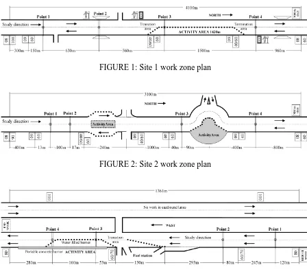
Page 6 of 20 diagrams of the work zones showing the posted speed limits and the location of the four speed measurement points are presented in Figures 1-3 (drawings not to scale). Standard sets of signage following the Manual of Uniform Traffic Control Devices (MUTCD)1 used in Queensland (Queensland Government, 2010) were used at all sites.It should be noted that vehicles travel on the left in Australia.
FIGURE 1: Site 1 work zone plan
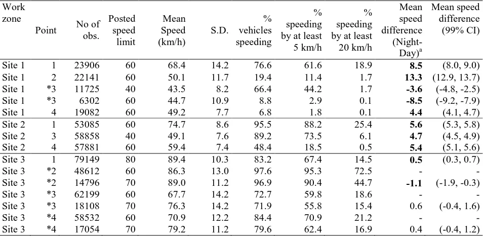
FIGURE 2: Site 2 work zone plan
FIGURE 3: Site 3 work zone plan
Site 1 was an undivided sealed two lane road (one lane each way) with pre-work speed limits of 100 km/h (southern end) and 80 km/h (northern end). The 4.1 km road section was straight and mostly flat with good sight distance. Average daily traffic volume was 3,415 vehicles with 74.9% of total traffic observed during daytime hours (6am – 6pm). Work (resurfacing) involved full closure of one lane within the activity area, with the closed lane alternating (southbound/northbound) as required. Traffic controller operated temporary traffic lights (and
1
Page 7 of 20 an additional traffic controller upstream to prevent vehicles queuing on bridge) were used to control traffic at each end of the activity area. Posted speed limit in the activity area was 40 km/h and 60 km/h during work hours (6am-6pm) and no-work hours, respectively.
At Site 2, work involved the addition of an extra lane in each direction to the existing two lanes (one each way). The pre-work speed limits were 90 km/h at the southern end of the work zone and 80 km/h at the northern end. The 3.1 km road section was flat with a mixture of straight sections and minor curves. Average daily traffic volume was 7,584 vehicles, of which 84.1% were observed during daytime hours. The activity area on the roundabout had a 40km/h limit all time, whereas the other activity area has 40 and 60 km/h during work hours and no-work hours respectively. With regard to removal and replacement of the 40/60 km/h signage, the research team could not be assured that the signage was always placed after data collection Point 2 by traffic controllers, as it was in the original plan. Therefore, data from Point 2 were subsequently excluded from analysis.
Site 3 comprised two lanes in each direction, divided by a 15 meter wide median, with 100 km/h pre-work speed limit. Average traffic volume was 11,307 vehicles per day, 79.5% of which were observed during daytime hours.Work involved construction of a new westbound slip lane exiting a fuel station, no traffic interruptions in the eastbound lanes. To allow vehicles exiting the fuel station merging on to through traffic, a second transition area was created after the standard transition area upstream. Field observation by authors showed that the vehicles exiting the fuel station comprised only a very small proportion of the through highway traffic. Therefore, any effects on the speeds of the overall traffic stream were considered negligible. The entire activity area was delineated by a water filled barrier, while the main work area was also protected by a portable concrete barrier. Speed limits in the activity area were changed from 60 km/h to 70 km/h at 6pm, and returned to 60 km/h at 6.30am for start of work day. In addition to the standard MUTCD signage, there was a fixed ‘Police Enforcement Zone’ sign, situated midway between data collection Points 1 and 2 (no enforcement was carried out during the data collection period).
4.2 Data collection and preparation
Speed data were collected using pairs of pneumatic tubes installed 1 meter apart on the pavement and connected to a MetroCount Vehicle Classification System. Travel speed, headway, gap, type of vehicle, and time were collected for each vehicle traversing the tubes over a continuous period of seven days. Vehicles were classified using the ARX vehicle classification scheme (MetroCount, 2009), which classifies vehicles into three aggregate classes: Light vehicles (Very short – bicycle, motorcycle; Short – sedan, wagon, 4WD, utility, light van; Short towing – trailer, caravan, boat etc.), Medium vehicles (two and three axle bus or truck, four axle truck), and Heavy vehicles (articulated vehicle or rigid vehicle and trailer with more than two axles, B-double or heavy truck and trailer, double or triple road train or heavy truck and more than one trailer). Data were collected and analyzed in metric units.
Page 8 of 20 removed. The northbound traffic in Sites 1 and 2 and westbound traffic in Site 3 were the directions of interest and speed data from these directions were analyzed in this study. Data points removed from this process were about 5.7%, 2.7%, and 12.5% of all observations at Sites 1, 2, and 3 respectively.
At Site 1, stop/slow traffic controls were located upstream of Points 2 and 3 during normal working hours. A careful examination of the data revealed that the first few vehicles in some stop/slow phases did not complete the acceleration process when starting from a stop
position, as indicated by increasing speeds of consecutive observations. Since these drivers did not reach their desired speed of travel when passing the tubes, it was necessary to remove those data points (7.8% of remaining data points). The final datasets include 83,156 (Site 1), 169,824 (Site 2), and 298,450 (Site 3) observations.
5. RESULTS
5.1 Descriptive statistics
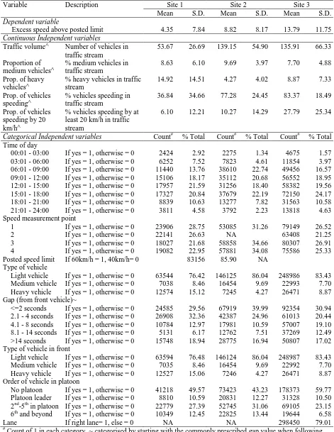
The collected speed data was first analyzed descriptively, in order to understand the general characteristics of speed profiles at the four locations in the work zones. The descriptive statistics of the speed profiles and magnitude of compliance with posted limits for the three work zones (Sites 1-3) are presented in the Table 1. It should be noted that the statistics were calculated for the directions of interest only (northbound in Site 1 and 2 and westbound in Site 3). Some points in Site 1 (point 3) and Site 3 (points 2, 3, and 4) had different speed limits during the day and night hours, so the statistics were presented separately for the speed limits. In order to determine if the speeds during night-time and daytime are different for a particular combination of work zone, measurement point, and speed limit, a two-sample t-test was employed for each of the combinations. Results of the t-tests are also presented in Table 1 by highlighting the results significant at 99% confidence level using bold faced numbers.
At all three sites, average speeds at Point 1 (after the first speed reduction sign) were higher than the posted speed limits. Compared to Points 2-4, the percentages of vehicles exceeding speed limits (both with small and large margins) were higher at Point 1. This indicates that motorists generally speed more in the upstream work zone areas.
Before the activity area at Site 3, there were two speed limit reductions: first to 80 km/h from 100 km/h at Point 1, and then to 60 km/h (day hours) or to 70 km/h (night hours) at Point 2. Comparison of the speeds at points after the reduced limits revealed that the average speeds were similar, regardless of the changed speed limits. In terms of proportion of vehicles speeding, about 83% exceeded the posted limit at Point 1, whereas almost all (about 97%) vehicles exceeded the limits at Point 2. These results suggest that the speed reduction signage in upstream work zone areas may have very limited effects on travel speeds.
Page 9 of 20 Table 1 Descriptive statistics of speed profiles and speed limit compliance
Work zone
Point No of
obs. Posted speed limit Mean Speed (km/h) S.D. % vehicles speeding % speeding by at least 5 km/h
% speeding by at least 20 km/h Mean speed difference (Night-Day)a Mean speed difference (99% CI)
Site 1 1 23906 60 68.4 14.2 76.6 61.6 18.9 8.5 (8.0, 9.0)
Site 1 2 22141 60 50.1 11.7 19.4 11.4 1.7 13.3 (12.9, 13.7)
Site 1 *3 11725 40 43.5 8.2 66.4 44.2 1.7 -3.6 (-4.8, -2.5)
Site 1 *3 6302 60 44.7 10.9 8.8 2.9 0.1 -8.5 (-9.2, -7.9)
Site 1 4 19082 60 49.2 7.7 6.8 1.8 0.1 4.4 (4.1, 4.7)
Site 2 1 53085 60 74.7 8.6 95.5 88.2 25.4 5.6 (5.3, 5.8)
Site 2 3 58858 40 49.1 7.6 89.2 73.5 6.1 4.7 (4.5, 4.9)
Site 2 4 57881 60 59.4 7.4 48.4 18.5 0.5 5.4 (5.1, 5.6)
Site 3 1 79149 80 89.4 10.3 83.2 67.4 14.5 0.5 (0.3, 0.7)
Site 3 *2 48612 60 86.3 13.0 97.6 95.3 72.5 - -
Site 3 *2 14796 70 89.0 11.2 96.9 90.4 44.7 -1.1 (-1.9, -0.3)
Site 3 *3 62199 60 67.7 14.2 72.7 59.8 18.6 - -
Site 3 *3 18108 70 76.3 14.2 71.9 55.8 15.4 0.6 (-0.4, 1.6)
Site 3 *4 58532 60 70.9 12.2 84.4 70.9 21.2 - -
Site 3 *4 17054 70 79.2 11.2 79.6 62.4 16.9 0.4 (-0.4, 1.2)
* Points with different speed limits during day and night periods, - No observation during night-time, Bold
values: significant at 99% confidence level, a H0: diff (mean night - mean day) = 0 with Ha: diff>0 (if diff is
positive) or Ha: diff<0 (if diff is negative)
At the end of activity area (Point 4), the average speed was higher than the posted speed limit at Site 3, but was lower at Site 1 and about equal at Site 2. About 80% of vehicles exceeded the limits at Site 3, whereas only 6.8% did so at Site 1. Although the average speed was almost equal to the posted limit at Site 2, about half of the vehicles still violated the posted speed limit, but mostly by small margins (18.5% had margins of 5 km/h or more). The night-time speeds were significantly higher than the daynight-time speeds at Site 1 (4.4 km/h) and Site 2 (5.4 km/h).
The average speed measured at a location downstream of a stop/slow traffic controller (Point 2) at Site 1 was lower than the posted limit of 60 km/h. However, 19% of vehicles were exceeding the limit with 11% exceeding by at least 5 km/h and 1.7% exceeding by at least 20 km/h. The average speed during night hours was significantly higher than during daytime. Furthermore, the difference between night and day speeds was higher here than at the other measurement points at this work zone. These findings might imply that motorists drive at lower speeds when passing a traffic controller standing on road, particularly during the day hours. While it is difficult to test with the available data, drivers’ difficulty in noticing traffic controllers during night hours might have contributed to the higher night-time speeds.
5.2 Regression model estimates
Page 10 of 20 conditions, separate models were estimated for each of the three work zones. It is worthy to note that the three work zones varied significantly in terms of traffic characteristics (average volumes were 3,415, 7,584, and 11,307 vehicles per day at Site 1, 2, and 3, respectively).
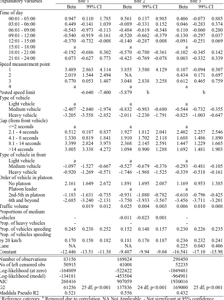
The summary statistics of the variables included in the models and the estimates of the model parameters along with their statistical significance are presented in Tables 2 and 3
respectively. Computed values for the change in the expected values of excess speed (amount of speed over the posted limit) for cases with positive values and the change in the probability of a driver’s speed being above the posted speed limit (expressed as percentage values) are presented in Table 4. Maddala Pseudo R2 values of the fitted Site 1 model, Site 2 model, and Site 3 model (0.52, 0.56, and 0.43 respectively) indicate good fit of the models. The
corresponding likelihood ratio statistics of the models are 61,256 (25 df), 137,836 (24 df), and 169,269 (26 df) respectively, which are well above the corresponding critical values for significance at 1% significance level, implying that the models have sufficient explanatory power.
Turning to the specific estimation results, relative to the 3-6pm hours, a lower percentage of vehicles were speeding during the other daytime hours (6am-3pm) at both Site 1 and Site 2. Marginal effects of the variables also showed smaller values for both the probability and magnitude of non-compliance during the 6am-3pm period. For example, a driver travelling at Site 1 during 6am-9am had 1.9% lower probability of exceeding the posted speed limit and the speed (if non-compliant with posted limit) is likely to be 0.1 km/h lower than the 3-6pm period. At Site 3, the results for only the 9am-12pm hours were statistically significant. During the early morning hours (12am-3am) all work zones saw higher magnitudes of speeding compared to the 3-6pm period. A driver had 7.3% and 3.5% higher probability of being non-compliant at Site 3 and Site 1 work zones respectively during the 12am-3am hours.
Relative to the end of the activity area (Point 4), the magnitudes of speeding at the other locations (i.e., start and upstream of activity area) were likely to be significantly higher (except at the Point 1 ‘after first speed reduction sign’ location of the Site 3 work zone where the difference was non-significant). The probability that a driver will be non-compliant was highest at Point 1 (after first speed reduction sign), for Site 1 (12.5%) and Site 2 (13.2%), with corresponding increases of 0.95 and 2.50 km/h in the excess speeds (i.e., amount of speed over the posted limit). After passing a stop/slow traffic controller (Point 2, Site 1 only), a driver is 7.0% more likely to exceed the posted speed limit. At the beginning of activity area (Point 3), the probabilities of exceeding speed limits were 2.6% (Site 1), 11.2% (Site 2), and 1.1% (Site 3) higher than those at the end of activity area.
Page 11 of 20 Table 2 Summary statistics of variables included in Tobit model
Variable Description Site 1 Site 2 Site 3
Mean S.D. Mean S.D. Mean S.D.
Dependent variable
Excess speed above posted limit 4.35 7.84 8.82 8.17 13.79 11.75
Continuous Independent variables
Traffic volume^ Number of vehicles in
traffic stream
53.67 26.69 139.15 54.90 135.91 66.33
Proportion of medium vehicles^
% medium vehicles in traffic stream
8.63 6.10 9.69 3.97 7.70 4.88
Prop. of heavy vehicles^
% heavy vehicles in traffic stream
14.92 14.51 4.27 4.02 8.87 7.33
Prop. of vehicles speeding^
% vehicles speeding in traffic stream
36.84 34.66 77.28 24.45 83.37 18.49
Prop. of vehicles speeding by 20 km/h^
% vehicles speeding by at least 20 km/h in traffic stream
6.10 12.21 10.27 14.29 27.79 25.34
Categorical Independent variables Count# % Total Count# % Total Count# % Total Time of day
00:01 - 03:00 If yes = 1, otherwise = 0 2424 2.92 2275 1.34 4675 1.57
03:01 - 06:00 If yes = 1, otherwise = 0 6252 7.52 7823 4.61 11854 3.97
06:01 - 09:00 If yes = 1, otherwise = 0 11440 13.76 38610 22.74 49456 16.57
09:01 - 12:00 If yes = 1, otherwise = 0 15106 18.17 35112 20.68 56552 18.95
12:01 - 15:00 If yes = 1, otherwise = 0 17957 21.59 31256 18.40 58382 19.56
15:01 - 18:00 If yes = 1, otherwise = 0 17327 20.84 37679 22.19 72150 24.17
18:01 - 21:00 If yes = 1, otherwise = 0 8839 10.63 13277 7.82 31563 10.58
21:01 - 24:00 If yes = 1, otherwise = 0 3811 4.58 3792 2.23 13818 4.63
Speed measurement point
1 If yes = 1, otherwise = 0 23906 28.75 53085 31.26 79149 26.52
2 If yes = 1, otherwise = 0 22141 26.63 NA 63408 21.25
3 If yes = 1, otherwise = 0 18027 21.68 58858 34.66 80307 26.91
4 If yes = 1, otherwise = 0 19082 22.95 57881 34.08 75586 25.33
Posted speed limit If 60km/h = 1, 40km/h= 0 83156 85.90 NA
Type of vehicle
Light vehicle If yes = 1, otherwise = 0 63544 76.42 146125 86.04 248986 83.43
Medium vehicle If yes = 1, otherwise = 0 7038 8.46 16454 9.69 22993 7.70
Heavy vehicle If yes = 1, otherwise = 0 12574 15.12 7245 4.27 26471 8.87
Gap (from front vehicle)~
<=2 seconds If yes = 1, otherwise = 0 24585 29.56 67919 39.99 92354 30.94
2.1 - 4 seconds If yes = 1, otherwise = 0 26908 32.36 42387 24.96 61013 20.44
4.1 - 8 seconds If yes = 1, otherwise = 0 10784 12.97 17981 10.59 57007 19.10
8.1 - 14 seconds If yes = 1, otherwise = 0 5131 6.17 12762 7.51 37269 12.49
>14 seconds If yes = 1, otherwise = 0 15748 18.94 28775 16.94 50807 17.02
Type of vehicle in front
Light vehicle If yes = 1, otherwise = 0 63594 76.48 146124 86.04 248987 83.43
Medium vehicle If yes = 1, otherwise = 0 7035 8.46 16454 9.69 22992 7.70
Heavy vehicle If yes = 1, otherwise = 0 12527 15.06 7246 4.27 26471 8.87
Order of vehicle in platoon
No platoon If yes = 1, otherwise = 0 41218 49.57 73423 43.23 178373 59.77
Platoon leader If yes = 1, otherwise = 0 8810 10.59 20831 12.27 31328 10.50
2nd-5th in platoon If yes = 1, otherwise = 0 22779 27.39 52745 31.06 69105 23.15
6th and beyond If yes = 1, otherwise = 0 10349 12.45 22825 13.44 19644 6.58
Lane If right lane= 1, else = 0 NA NA 298450 79.01
# Count of 1 in each category, ~ categorised by starting with the commonly prescribed gap value when following
Page 12 of 20 Table 3 Tobit regression estimates
Explanatory variables Site 1 Site 2 Site 3
Beta 99% CI Beta 99% CI Beta 99% CI
Time of day
00:01 - 03:00 0.947 0.110 1.785 0.561 0.137 0.985 0.406 -0.073 0.885
03:01 - 06:00 0.449 -0.141 1.039 -0.089 -0.331 0.152 0.046 -0.283 0.374
06:01 - 09:00 -0.543 -0.973 -0.113 -0.484 -0.619 -0.348 0.110 -0.060 0.280
09:01 - 12:00 -0.540 -0.919 -0.161 -0.520 -0.662 -0.379 -0.130 -0.297 0.037
12:01 - 15:00 -0.370 -0.732 -0.008 -0.140 -0.287 0.008 -0.091 -0.251 0.069
15:01 - 18:00 a a a
18:01 - 21:00 -0.192 -0.686 0.302 -0.570 -0.780 -0.361 -0.102 -0.345 0.142
21:01 - 24:00 0.073 -0.627 0.773 -0.423 -0.769 -0.078 0.003 -0.332 0.339
Speed measurement point
1 3.489 2.863 4.114 3.855 3.580 4.129 0.107 -0.094 0.307
2 2.019 1.544 2.494 NA 0.434 0.171 0.697
3 0.770 0.053 1.487 3.048 2.838 3.258 0.612 0.465 0.759
4 a a a
Posted speed limit -6.640 -7.400 -5.879 b b
Type of vehicle
Light vehicle a a a
Medium vehicle -2.407 -2.840 -1.974 -0.832 -0.983 -0.680 -0.544 -0.732 -0.355
Heavy vehicle -3.205 -3.558 -2.852 -2.011 -2.230 -1.791 -0.825 -1.003 -0.647
Gap (from front vehicle)
<=2 seconds a a a
2.1 - 4 seconds 0.512 0.187 0.837 1.927 1.812 2.041 2.402 2.257 2.546
4.1 - 8 seconds 1.330 0.819 1.841 1.910 1.702 2.118 1.688 1.486 1.890
8.1 - 14 seconds 3.399 2.824 3.973 2.368 2.145 2.591 1.447 1.229 1.665
>14 seconds 3.805 3.338 4.272 1.094 0.900 1.288 1.692 1.481 1.903
Type of vehicle in front
Light vehicle a a a
Medium vehicle -1.097 -1.527 -0.667 -0.527 -0.679 -0.376 -0.293 -0.481 -0.105
Heavy vehicle -0.920 -1.269 -0.571 -1.746 -1.968 -1.525 -0.339 -0.518 -0.161
Order of vehicle in platoon
No platoon 2.161 1.649 2.672 1.891 1.695 2.087 1.169 0.953 1.385
Platoon leader a a a
2nd-5th in platoon -1.183 -1.631 -0.735 -0.931 -1.080 -0.782 -0.610 -0.796 -0.425
6th and beyond -2.685 -3.240 -2.131 -3.750 -3.933 -3.567 -3.456 -3.711 -3.201
Traffic volume 0.019 0.012 0.025 0.004 0.003 0.006 0.010 0.008
Proportions of medium
vehicles - -0.011 -0.023 0.001 -
Prop. of heavy vehicles - - -
Prop. of vehicles speeding 0.245 0.238 0.252 0.152 0.148 0.157 0.230 0.226 0.235
Prop. of vehicles speeding
by 20 km/h 0.170 0.158 0.182 0.181 0.176 0.187 0.236 0.232 0.241
Lane NA NA 0.225 0.043 0.406
Constant -12.446 -13.51 -11.38 -9.487 -9.94 -9.04 -16.541 -17.10 -15.98
Number of observations 83156 169824 298450
No of left censored obs 50915 41008 52235
Log-likelihood (at zero) -164809 -522422 -1049481
Log-likelihood (model) -134181 -453504 -964981
AIC 268416 907059 1930016
G2 61256 25 df; p<0.001 137836 24 df; p<0.001 169000 25 df; p<0.001
Maddala Pseudo R2 0.521 0.556 0.432
a
Reference category, b Removed due to correlation, NA Not Applicable, - Not significant at 95% confidence
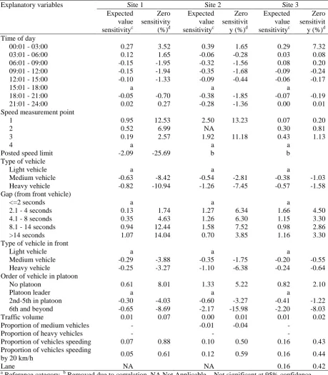
Page 13 of 20 Table 4 Marginal effects of estimated Tobit regression parameters
Explanatory variables Site 1 Site 2 Site 3
Expected value sensitivityc Zero sensitivity (%)d Expected value sensitivityc Zero sensitivit
y (%)d
Expected value
sensitivityc
Zero sensitivit
y (%)d
Time of day
00:01 - 03:00 0.27 3.52 0.39 1.65 0.29 7.32
03:01 - 06:00 0.12 1.65 -0.06 -0.28 0.03 0.08
06:01 - 09:00 -0.15 -1.95 -0.32 -1.56 0.08 0.20
09:01 - 12:00 -0.15 -1.94 -0.35 -1.68 -0.09 -0.24
12:01 - 15:00 -0.10 -1.33 -0.09 -0.44 -0.06 -0.17
15:01 - 18:00 a a a
18:01 - 21:00 -0.05 -0.70 -0.38 -1.85 -0.07 -0.19
21:01 - 24:00 0.02 0.27 -0.28 -1.36 0.00 0.01
Speed measurement point
1 0.95 12.53 2.50 13.23 0.07 0.20
2 0.52 6.99 NA 0.30 0.81
3 0.19 2.57 1.92 11.18 0.43 1.13
4 a a a
Posted speed limit -2.09 -25.69 b b
Type of vehicle
Light vehicle a a a
Medium vehicle -0.63 -8.42 -0.54 -2.81 -0.38 -1.03
Heavy vehicle -0.82 -10.94 -1.26 -7.45 -0.57 -1.58
Gap (from front vehicle)
<=2 seconds a a a
2.1 - 4 seconds 0.13 1.74 1.27 6.34 1.66 4.50
4.1 - 8 seconds 0.35 4.63 1.26 6.30 1.15 3.30
8.1 - 14 seconds 0.94 12.44 1.58 7.52 0.98 2.86
>14 seconds 1.07 14.04 0.70 3.85 1.16 3.30
Type of vehicle in front
Light vehicle a a a
Medium vehicle -0.29 -3.88 -0.35 -1.75 -0.20 -0.55
Heavy vehicle -0.25 -3.27 -1.10 -6.38 -0.24 -0.64
Order of vehicle in platoon
No platoon 0.61 8.01 1.33 5.22 0.82 2.10
Platoon leader a a a
2nd-5th in platoon -0.30 -4.03 -0.60 -3.27 -0.41 -1.22
6th and beyond -0.65 -8.69 -2.17 -15.98 -2.20 -8.03
Traffic volume 0.01 0.07 0.00 0.01 0.01 0.02
Proportion of medium vehicles - -0.01 -0.04 -
Proportion of heavy vehicles - - -
Proportion of vehicles speeding 0.07 0.88 0.10 0.50 0.16 0.43
Proportion of vehicles speeding
by 20 km/h 0.05 0.61 0.12 0.59 0.16 0.44
Lane NA NA 0.16 0.42
a
Reference category, b Removed due to correlation, NA Not Applicable, - Not significant at 95% confidence
level, c Change in the expected value of excess speed (for cases above zero, i.e., speeding cases), d Change in the
probability of being above zero (i.e., exceeding posted speed limits)
Page 14 of 20 of the following vehicle being non-compliant was smaller when following a medium vehicle (Site 1: 3.9%; Site 2: 1.8%; Site 3: 0.5%) or following a heavy vehicle (Site 1: 3.3%; Site 2: 6.4%; Site 3: 0.6%). These results demonstrate that the speed of a particular vehicle and the probability of it exceeding the posted limits not only depend on its type but also on the type of vehicle it is following.
The effect of a driver’s freedom to travel at his/her desired speed of travel was captured in the models using the gap variable which expresses the time difference between the front wheels of each vehicle and the rear wheels of its leader vehicle at the point of speed measurement. Relative to the vehicles with a small gap to the vehicles in front (<= 2 seconds which is usually prescribed to drivers as the safe gap value for following another vehicle—see SWOV, 2012 for details), vehicles with larger gaps were more likely to travel at higher speeds and to exceed the posted speed limits. For instance, at Site 1 the probability of being non-compliant was 1.7% higher when the gap was 2.1 to 4 seconds, 4.6% higher when the gap was 4.1 to 8 seconds, 12.4% higher when the gap was 8.1 to 14 seconds, and 14.0% higher when the gap was greater than 14 seconds. The results were consistent among all three work zones studied.
The platoon variable (expressed in four categories in terms of the position of a vehicle in a platoon, if there is one) was included in the models to capture the effects of platoons on travel speeds. A platoon is defined as a group of vehicles (two or more) travelling close to one other with headway (time difference between the passing of the front wheels of two consecutive vehicles over a particular point) of less than or equal to 4 seconds, as used in many studies (e.g., Hajbabaie et al., 2011b; Sun and Benekohal, 2005). The results showed that the effects of platoon rank and travelling outside of a platoon were consistent across all work zones. Relative to the leaders of platoons, the follower vehicles had lower magnitudes and
probabilities of non-compliance. The vehicles in a platoon with 2nd to 5th rank (considering the leader of the platoon as ranked 1st) and those in the tails of platoons (ranks 6th and
beyond) had lower probabilities of being non-compliant (Site 1: 4.0% and 8.7%; Site 2: 3.3% and 16%; Site 3: 1.2% and 8.0%). On the other hand, vehicles not in a platoon had higher probabilities of being non-compliant (Site 1: 8.0%; Site 2: 5.2%; Site 3: 2.1%) than the leaders of platoons.
The foregoing shows that type of leader vehicle, gap from a leader vehicle, and order of a vehicle in a platoon affects travel speeds of vehicles. Other characteristics of surrounding traffic, such as traffic volume, proportions of different types of vehicles, and proportions of vehicles speeding may also influence travel speeds. These variables were defined in 15 minute blocks around the time when a vehicle’s speed was measured. The results showed that a unit increase in traffic volume (number of vehicles in 15 minute period) was associated with an increase in the amount of excess speed and the probability of exceeding posted speed limits by 0.005 km/h and 0.07% (Site 1), 0.003 km/h and 0.01% (Site 2), and 0.007 km/h and 0.02% (Site 3) respectively. The proportion of medium vehicles was found significant for the Site 2 work zone only, which showed that 1% increment in the proportion of medium
vehicles in a 15 minute block was associated with a 0.007 km/h decrease in excess speed and a 0.04% decrease in the probability of being non-compliant.
Page 15 of 20 surrounding traffic was associated with 0.9% increase in the probabilities of other vehicles violating the speed limits. The corresponding values for Sites 2 and 3 work zones were 0.5% and 0.4% respectively. In the case of a 1% increase in proportion of vehicles exceeding the posted limits by a margin of 20 km/h or more in the surrounding traffic, the probabilities of others vehicles being non-compliant were increased by 0.6%, 0.6%, and 0.4% for Sites 1, 2 and 3 respectively. These results indicate that a driver’s speed at a particular point is significantly influenced by the speed profiles of other drivers travelling through the same point in a short time interval (in this case 15 minutes).
Only Site 3 had two lanes travelling in the same direction. As expected, the speeds in the right lane were higher, with 0.4% higher probability of a vehicle being non-compliant than in the left lane.
6. DISCUSSION
The current study offers important new insights for work zone speed data analysis. The successful application to analyze speed data at three separate work zones with different traffic characteristics in the current study validates the use of the Tobit regression model. All three models produced similar results in demonstrating the influence of surrounding traffic on vehicle speeds. The model showed that a vehicle is more likely to speed in higher traffic volumes, where there are high proportions of other vehicles speeding, and where other vehicles are speeding by a large margin. Vehicles not in a platoon and the leaders of platoon were more likely to speed than those in the middle of a platoon. Independent of platoons, speeding was more likely where larger gaps exist. The estimated regression coefficients and their marginal effects on both the amount of excess speed and the probability of a driver being non-compliant were consistent and of plausible signs across the three work zones studied. Importantly, the modeling technique used is transferrable and may be applied in a wide range of studies to examine vehicle speeds and to evaluate effectiveness of speed-reduction countermeasures, both within work zones and elsewhere in the general road network. In doing before-after studies of speed reduction countermeasures, special considerations need to be given to any potential site-selection effects, as demonstrated by Kuo and Lord (2013).
Page 16 of 20 In upstream work zone areas, both the amount of non-compliance (proportion of vehicles speeding) and the magnitude of speeding (amount over the limit) were found to be greatest among all locations studied. Accordingly, as also found in other research (e.g., Benekohal et al.,1992; Brewer et al., 2006), drivers in the current study were relatively more compliant in close proximity to active work areas, indeed where speed limits are lowest and a large proportion of serious and fatal injuries are most likely to occur (FMCSA, 2002; Mohan and Zech, 2005). While the greater compliance is thus somewhat positive, the degree of non-compliance (44-73% exceeded the limits by at least 5 km/h) nonetheless remains a concern.
The current study also found that the presence of a traffic controller had a notable effect in reducing speeds. After passing a traffic controller (Point 2 of Site 1), most vehicles complied with the posted limit and only 20% exceeded the limit on average at this point. However, the difference between day and night speeds was found to be the greatest at this location (after the traffic controller), suggesting a possible issue with reduced visibility of traffic controllers at night.
Compared to upstream areas, speeding was found to be somewhat less prevalent toward the end of work zones. Speeding was most evident at Site 3, at which there are two lanes travelling in the direction of study under normal conditions, compared with only one lane at Sites 1 and 2. This difference may have influenced a greater amount of speeding towards the end of the Site 3 work zone. Wang et al. (2003) have reported substantial initial speed reductions followed by subsequent increases in the advance warning area, before further reductions at the activity area. The current study’s Site 3 observation of no speed difference over two speed limit reductions in the advance warning area suggests a similar approach by drivers, whereby they tend to react more upon seeing activity than they do to posted speed limits. As previously reported, drivers tend to navigate work zones at a speed with which they are comfortable, rather than strictly adhering to posted limits (Brewer et al., 2006; Haworth et al., 2002).
Comparing the three work zones in the current study, across the length of each entire work zone, non-compliance was greater at Site 3 than at Sites 1 or 2. As noted above, on approach to the Site 3 activity area, there was no speed difference observed over two speed limit reductions. On exiting the activity area, speeding was again most common and of greatest magnitude at Site 3. One of the major differences between Site 3 and the other sites was that Site 3 was a divided highway with two lanes in each direction whereas the other sites were on two-lane undivided highways. Although traffic volumes were higher at Site 3 than other sites, these volumes were accommodated over 2 lanes. While pre-work speed limits were similar at all three sites, two lanes therefore approached the Site 3 activity area as opposed to one lane at Sites 1 and 2. This may have contributed to the higher speeds and lower compliance at Site 3 through larger gaps and less platoon effects on vehicle speeds.
Page 17 of 20 bearing in mind that these areas do not necessarily coincide. The possibility that
countermeasure deployment and greater compliance upstream of an activity area will also have significant downstream effects (Medina et al., 2009) should be considered in this regard. In addition to highlighting the prevalence of speeding in particular work zone areas, other specific situations in which vehicles are more or less likely to speed, such as time of day for example, are also could be useful for targeted enforcement.
This study was limited to illustration of the modeling technique in examining speed limit non-compliance at long-term work zones on national highways. Care should be taken when transferring the findings to other contexts, including short-term work zones and urban roads with relatively low pre-work speed limits for example. From an analysis of driver casualty risk in different types of work zones, Weng and Meng (2011) showed that the risk factors (e.g., day of week, gender of driver) have different effects on casualty risk for different types of work zones. The modeling technique illustrated in this paper could however effectively be applied to speed limit compliance modeling in any types of work zones. In using the
modeling technique, future work zone speed modeling should focus on three important issues (1) analyzing the effects of driver characteristics on speeds (Weng and Meng, 2012 showed that driver characteristics have significant effects on risky driving behavior including
speeding), (2) investigating if work zone geometric characteristics have significant influences on speeds, and (3) examining the potential correlations among speeds of same vehicles measured at different locations. Investigating the second issue is possible by conducting a large scale study involving many work zones of different geometric configuration (e.g., lane width, lane closure, taper length, horizontal and vertical alignment etc.). However, examining the first issue would require conducting a designed experiment in which individual drivers are identifiable in the speed dataset (possibly using a driving simulator). To investigate the third issue—whether the speeds of same vehicles at different locations are temporally
correlated—it is necessary to collect some form of vehicle IDs with speed data so that speeds of each vehicle can be tracked. However, this was not possible to do in the current study, because pneumatic tube counters were used to collect speed data. While these counters do not collect any vehicle IDs, they are capable of collecting speed and gap data of all vehicles (so it was possible to identify the platoons and examine their effects on speed limit compliance). It is to be noted that the extensions of the current paper proposed here would require significant data collection efforts which were beyond the scope of the current study. The scope was essentially limited to demonstrating the applicability and validity of the Tobit modeling technique for advancing the methodological development in analyzing work zone speed data.
7. CONCLUSIONS
This paper presented a new technique for modeling speed limit compliance in work zones to understand the how different vehicle and traffic related factors influence speed limit
compliance. The technique, which is capable of accounting for both the probability and magnitude of non-compliance, was illustrated using speed data obtained from three long-term highway work zones in Australia. Modeling estimates across the fitted models for the three work zones were consistent and of plausible sign which supports the appropriateness and validity of the modeling technique.
Page 18 of 20 vehicles and those following a light vehicle, vehicles with larger gaps from leader vehicle, leaders of platoons and those not in a platoon had higher probabilities of being non-compliant with larger margins above the posted speed limits. Higher traffic volumes and higher
proportions of non-compliant vehicles in the surrounding traffic were also associated with a higher likelihood and magnitude of non-compliance. Motorists generally speed more in the upstream work zone areas than in the activity area, and upstream speed reduction signage may have limited effects on speed choice. Significant rates of speeding were observed at the start of activity areas, but speeding was found to be less prevalent toward the end of activity area in comparison with other parts of work zones. Motorists were generally compliant when passing a stop/slow traffic controller, particularly during the day. Reduced visibility of traffic controllers during night-time may have contributed to the significant difference between the day and night speeds at this location.
Apart from understanding work zone speed profiles, the modeling technique developed has potential for use in evaluations of the effectiveness of speed-control measures in work zones or in other segments of a road network. Incorporation of driver and work zone geometric characteristics in the modeling framework to understand how these characteristics affect motorists’ speed choice would be a valuable addition in future research.
ACKNOWLEDGEMENTS
The authors are grateful to Australian Research Council, GHD Pty Ltd, Leighton Contractors, and QLD Department of Transport and Main Roads for funding the research project titled “Integrating Technological and Organisational Approaches to Enhance the Safety of Roadworkers” (Grant No. LP100200038). The authors would also like to acknowledge the support of the Australian Workers Union. Special thanks go to Mr Colin Edmonston of Transport and Main Roads for his kind assistance in facilitating data collection. The comments expressed in this paper are those of the authors and do not necessarily represent the policies of these organizations.
REFERENCES
Aarts, L., van Schagen, I., 2006. Driving speed and the risk of road crashes: A review. Accident Analysis & Prevention38 (2), 215-224.
Allpress, J.A., Leland Jr, L.S., 2010. Reducing traffic speed within roadwork sites using obtrusive perceptual countermeasures. Accident Analysis & Prevention42 (2), 377-383.
Bai, Y., Finger, K., Li, Y., 2010. Analyzing motorists' responses to temporary signage in highway work zones. Safety Science48 (2), 215-221.
Bai, Y., Li, Y., 2011. Determining the drivers' acceptance of EFTCD in highway work zones. Accident Analysis & Prevention43 (3), 762-768.
Benekohal, R.F., Hajbabaie, A., Medina, J.C., Wang, M., Chitturi, M.V., 2010. Speed photo-radar enforcement evaluation in Illinois work zones. Report No. FHWA-ICT-10-064, Illinois Center for Transportation, Urbana.
Benekohal, R.F., Wang, L., Orloski, R.L., Kastel, L.M., 1992. Speed Reduction Profiles of Vehicles in a Highway Construction Zone. Report No. FHWA/IL/UI-241, Department of Civil Engineering, University of Illonis at Urbana-Chapaign, Urbana-Champaign. Bham, G.H., Mohammadi, M.A., 2011. Evaluation of work zone speed limits: An objective
Page 19 of 20 Brewer, M.A., Pesti, G., Schneider, W., 2006. Improving compliance with work zone speed
limits: Effectiveness of selected devices. Transportation Research Record1948, 67-76.
Daniel, J., Dixon, K., Jared, D., 2000. Analysis of fatal crashes in Georgia work zone. Transportation Research Record1715, 18-23.
Debnath, A.K., Blackman, R., Haworth, N., 2013. Understanding worker perceptions of common incidents at roadworks in Queensland. In: Proceedings of the 2013 Australasian Road Safety Research, Policing & Education Conference, Brisbane, Australia.
Debnath, A.K., Blackman, R.A., Haworth, N., 2014. Effectiveness of pilot car operations in reducing speeds in a long-term rural highway work zone. In: Proceedings of the Transportation Research Board Annual Meeting 2014, Washington, DC.
Debnath, A.K., Blackman, R.A., Haworth, N.L., 2012. A review of the effectiveness of speed control measures in roadwork zones. In: Proceedings of the Occupational Safety in Transport Conference, Gold Coast, Australia.
FHWA, 2009. Manual on uniform traffic control devices for streets and highways. In: Federal Highway Administration, U.S.D.O.T. ed., Washington D.C.
FMCSA, 2002. 2000 Work Zone Traffic Crash Facts. Federal Motor Carrier Safety Administration, Washington D.C.
Garber, N.J., Zhao, M., 2002. Crash characteristics at work zones. Report No. FHWA/VTRC 02-R12, Virginia Transportation Research Council, Charlottesville.
Hajbabaie, A., Medina, J.C., Wang, M.-H., Benekohal, R.F., Chitturi, M., 2011a. Sustained and Halo Effects of Various Speed Reduction Treatments in Highway Work Zones. Transportation Research Record2265, 116-126.
Hajbabaie, A., Ramezani, H., Benekohal, R.F., 2011b. Speed Photo Enforcement Effects on Headways in Work Zones. In: Proceedings of the Transportation and Development Institute Congress 2011, pp. 1226-1234.
Haworth, N., Symmons, M., Mulvihill, C., 2002. Safety of small workgroups on roadways. Report No. 195, Monash University Accident Research Centre, Melbourne.
Kuo, P.-F., Lord, D., 2013. Accounting for site-selection bias in before-after studies for continuous distributions: Characteristics and application using speed data. Trnasportation Researh Part A 49, 256-269.
Li, Y., Bai, Y., 2008. Comparison of characteristics between fatal and injury accidents in the highway construction zones. Safety Science46 (4), 646-660.
Medina, J.C., Benekohal, R.F., Hajbabaie, A., Wang, M.-H., Chitturi, M.V., 2009.
Downstream Effects of Speed Photo–Radar Enforcement and Other Speed Reduction Treatments on Work Zones. Transportation Research Record2107, 24-33.
Meng, Q., Weng, J., Qu, X., 2010. A probabilistic quantitative risk assessment model for the long-term work zone crashes. Accident Analysis and Prevention 42 (6), 1866-1877. MetroCount, 2009. Classification Schemes: MTE User Manual. MetroCount.
Mohan, S., Zech, W.C., 2005. Characteristics of worker accidents on NYSDOT construction projects. Journal of Safety Research36 (4), 353-360.
Morgan, J.F., Duley, A.R., Hancock, P.A., 2010. Driver responses to differing urban work zone configurations. Accident Analysis & Prevention42 (3), 978-985.
Queensland Government, 2010. Manual of uniform traffic control devices - Part 3: Works on roads. In: Department of Transport and Main Roads ed., Brisbane.
Sun, D., Benekohal, R.F., 2005. Analysis of work zone gaps and rear-end collision probability. Journal of Transportation and Statistics8 (2), 71-86.
Page 20 of 20 Tobin, J., 1958. Estimation of relationships for limited dependent variables. Econometrica26
(1), 24-36.
Wang, C., Dixon, K.K., Jared, D., 2003. Evaluation of Speed Reduction Strategies for Highway Work Zones. In: Proceedings of the 82nd Annual Meeting of the Transportation Research Board, Washington, D.C.
Washington, S.P., Karlaftis, M.G., Mannering, F.L., 2011. Statistical and econometric methods for transportation data analysis (second edition) CRC Press, Chanpman and Hall.
Weng, J., Meng, Q., 2011. Analysis of driver casulaty risk for different work zone types. Accident Analysis and Prevention 43 (5), 1811-1817.